Moving lattice kinks and pulses: an inverse method

Abstract

We develop a general mapping from given kink or pulse shaped travelling-wave solutions including their velocity to the equations of motion on one-dimensional lattices which support these solutions. We apply this mapping - by definition an inverse method - to acoustic solitons in chains with nonlinear intersite interactions, to nonlinear Klein-Gordon chains, to reaction-diffusion equations and to discrete nonlinear Schrödinger systems. Potential functions can be found in at least a unique way provided the pulse shape is reflection symmetric and pulse and kink shapes are at least $C^{2}$ functions. For kinks we discuss the relation of our results to the problem of a Peierls-Nabarro potential and continuous symmetries. We then generalize our method to higher dimensional lattices for reaction-diffusion systems. We find that increasing also the number of components easily allows for moving solutions.

I Introduction

Finding exact travelling-wave (TW) solutions of nonlinear lattice systems has been a problem of growing interest in recent years. Apart from some integrable systems which support TW solutions (e.g., [1]), a little is known about non-integrable discrete systems. It appears to be difficult to prove the existence of such waves because one has to deal with differential equations with advance and delay terms (on some general properties of these equations see [2]). The existence of acoustic (pulse) solitary waves as travelling-wave solutions in lattices with nonlinear intersite interactions has been proved in [3]. However, no proof is available for other types of solitary waves, for instance, topological solitons in nonlinear Klein-Gordon (KG) lattices or other discrete kink-bearing systems (an exception is given in [4]). Stationary breathers have been shown to be generic solutions for lattice systems (for a review and further references see [5]). Again the question of whether moving breathers on lattices exist is still not answered, although a number of approaches to the subject are known [6],[7],[8],[9], [10],[11]). An exception is the case of the integrable Ablowitz-Ladik equation [12].

Here we approach the TW existence problem from the inverse side - we show that for a given TW profile, corresponding equations of motion can be generated, so that these equations of motion yield the chosen TW profile as a solution. This has been done first in [13] for the $\tanh$-shaped kink and extended to reaction-diffusion-type systems in [14]. However, in both cases the analysis was performed for a specific class of profiles, whereas we will approach this problem from a general point of view. This in turn will allow us to obtain general information about the properties of the TW solutions.

The structure of the paper is as follows. In Section II we introduce the equations of motion. Section III is devoted to solutions of the nonlinear Klein-Gordon equation and of reaction-diffusion-type systems. In Section IV we study chains with nonlinear intersite interactions which admit acoustic (pulse) soliton solutions. We will refer to this type of lattices as to acoustic chains. In Section V we deal with discrete nonlinear Schrödinger-type (DNLS) equation. Section VI is devoted to the structural stability of solitary waves, and Section VII generalizes our method to higher space dimensions. Conclusions are given in Section VIII.

II The equations of motion

We consider a one-dimensional chain with lattice spacing equal to unity, which describes a system of interacting particles of unity mass. Such a system has a direct physical meaning and can describe, for example, simple quasi-one-dimensional molecular crystals. The interparticle interaction potential $W_{n-n^{\prime}}(r)$ and the on-site potential $V(u)$ are, in general, nonlinear functions:

$${\ddot{u}}_{n}=-V^{\prime}(u_{n})+\sum_{m}W_{n-m}^{\prime}(u_{n}-u_{m})$$ (1)

where $u_{n}$ is the displacement of the $n$th particle from its equilibrium position and $m,n$ are integers. If the second derivative $\ddot{u}$ in Eq. (1) is replaced by the first derivative $\dot{u}$, we obtain a system of reaction-diffusion equations.

Another system of interest is a generalized discrete nonlinear Schrödinger equation (DNLS)

$$i{\dot{\phi}}_{n} + C(\phi_{n+1}-2\phi_{n}+\phi_{n-1})$$ (2)

$$+ F(|\phi_{n}|^{2})(\phi_{n-1}+\phi_{n+1})+G(|\phi_{n}|^{2})\phi_{n}=0~{}$$ (3)

which appears in various fields. Here $\phi_{n}(t)$ is a complex-valued function and $F$ and $G$ are general nonlinear functions.

We are not aware of any systematic approach which shows the existence or even obtains analytical expressions for TW solutions of the equations from above. Therefore we approach the problem from the opposite side. We formulate an inverse method of creating the potentials $V$ or $W$ or the pair of functions $(F,G)$ for a given TW solution.

III Solutions of the nonlinear Klein-Gordon equation

For sake of simplicity let us consider the case of harmonic intersite interaction $W_{n-n^{\prime}}(r)=(Cr^{2}/2)\delta_{n,(n^{\prime}\pm 1)}$. Then the equation of motion (1) becomes the well-known nonlinear Klein-Gordon equation:

$$\ddot{u}_{n}=C(u_{n+1}-2u_{n}+u_{n-1})-V^{\prime}(u_{n}).$$ (4)

First, let us study the dispersion law for small-amplitude waves oscillating around some minimum $u_{min}$ of the potential $V(u)$. After linearising the on-site potential around the above-mentioned minimum the dispersion law can be written as follows

$$\omega_{q}^{2}=\gamma+2C(1-\cos{q})$$ (5)

where $q$ is a wave number and $\gamma=V^{\prime\prime}(u_{min})$. The group velocity $s_{0}=\partial\omega_{q}/\partial q$ attains its maximal value $s_{max}$ when $\partial s_{0}/\partial q=0$:

$$s_{max}=\sqrt{C-\frac{\sqrt{\gamma^{2}+4\gamma C}-\gamma}{2}}~{}.$$ (6)

We are interested in TW solutions, i.e., solutions that propagate with a permanent shape and velocity:

$$u_{n}(t)=u(n-st)\equiv u(z)~{},~{}~{}~{}z=n-st~{},$$ (7)

where $s$ is the velocity of the travelling wave. As a result, we obtain a differential equation with delay and advance terms:

$$s^{2}u^{\prime\prime}(z)=C[u(z+1)-2u(z)+u(z-1)]-V^{\prime}[u(z)]\;\;.$$ (8)

A Moving pulses

First we consider solutions of a bell-shaped localized form, i.e., pulses. Given the profile $u(z)$ and its velocity $s$, we can generate the on-site potential $V$. The function $u(z)$ should satisfy the following conditions:

• $u(z\rightarrow\pm\infty)\rightarrow 0$

• $u(-z)=u(z)$

• $u(z)$ is monotonic in $[0,+\infty[$

• $u(z)$ is analytic in $[0,+\infty[$   .

To show that the potential $V$ can be generated in a unique way, we rewrite Eq. (8) in the following form:

$$V^{\prime}[u(z)] \equiv f[u(z)]=-s^{2}u^{\prime\prime}(z)$$ (9)

$$+ C[u(z+1)-2u(z)+u(z-1)]\;\;.$$ (10)

Now we see that there exists a unique correspondence between the function $u(z)$ and the force function $f(u)$. Since $u(z)$ is analytic, we can always rewrite $u(z\pm 1)$ in terms of $u(z)$. Therefore for each $u(z)$ with the conditions listed above the function $f(u)$ can be uniquely defined. The potential $V$ is then obtained by integrating $f(u)$ once. This result does not change if we consider a more complicated interaction potential $W$ which incorporates anharmonic terms and long range interactions. Thus, we showed here, that for a given interaction potential $W$, a given pulse profile $u(z)$ which satisfies the above conditions and a given velocity of the pulse we always generate a unique on-site potential $V$ which supports this TW profile as an exact solution of the equations of motion.

What would happen if we loose the symmetry condition on $u(z)$? Consider two values $z_{1},z_{2}$ at which $u(z_{1})=u(z_{2})$. Consequently, the argument of the force function is also the same. But the rhs of Eq. (10) will be different for $z_{1}$ and $z_{2}$ in general, which implies that we obtain two different values for the force function at the same argument - a circumstance impossible for standard functions. Thus, we have to require the symmetry of $u(z)$ which guarantees that the force function is defined in a unique way. This is also the reason why we can exclude the existence of more complicated pulse forms like anti-symmetric pulses, symmetric pulses with several maxima etc.

Let us investigate some properties of $V$. Since for $z\rightarrow\infty$ $u\rightarrow 0$ and $u^{\prime\prime}\rightarrow 0$, we find that $f(0)=0$ which was to be expected. To get more information about the dependence of $f(u)$ for small $u$ (which tells us about the stability of the TW solution) we need the leading order dependence of $u$ on $z$ for large $z$ which is given by the ansatz of the TW profile. Let us assume that our ansatz yields an exponential decay of $u(z)$ for large distances, i.e.,

$$u(z\rightarrow\pm\infty)\sim e^{-\mu|z|}~{},~{}~{}\mu>0~{}.$$ (11)

After substituting Eq. (11) into Eq. (10) we obtain

$$f(u)\simeq-u[\mu^{2}s^{2}-2C(\cosh\mu-1)]~{}.$$ (12)

The slope of the force $f(u)$ for small $u$ changes its sign when $C$ crosses the value $C_{1}$ given by

$$C_{1}=\frac{s^{2}\mu^{2}}{2(\cosh\mu-1)}.$$ (13)

This means that the potential $V(u)$ has maxima at $u=0$ when $C<C_{1}$ and minima if $C>C_{1}$. Consequently, the asymptotic state $u(z\rightarrow\pm\infty)=0$ is a dynamically unstable one for $C<C_{1}$ and a stable one for $C>C_{1}$. There is another critical value [see again Eq. (10)] of $C$ given by

$$C_{2}=\frac{s^{2}u^{\prime\prime}(0)}{2[u(1)-u(0)]}~{}.$$ (14)

If $C>C_{2}$, an additional extremum (maximum) in $V(u)$ appears between $u=0$ and $u(0)$. The possible scenarios $C_{1}<C_{2}$ and $C_{1}>C_{2}$ are shown in Fig. 1(a) and Fig. 1(b), respectively. The above statements about stability hold for any exponentially decaying pulse. If the decay is non-exponential, the on-site potential can become non-analytic at $u=0$. For example, for a Gaussian tail

$$u(z\rightarrow\pm\infty)\sim e^{-\mu z^{2}}$$ (15)

the on-site potential for small $u$ gets dressed with logarithmic corrections, e.g. for $\mu=1$

$$f(u)=V^{\prime}(u) \simeq u\left[-s^{2}(2+4\ln u)\right.$$ (16)

$$+ \left.2C-\frac{2C}{e}\cosh\left(2\sqrt{-\ln{u}}\right)\right]~{}.$$ (17)

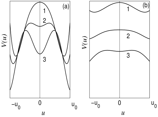
FIG. 1.: The potential $V(u)$ for a fixed pulse solution: (a) for $C_{1}<C_{2}$ and 1: $C<C_{1}<C_{2}$, 2: $C_{1}<C<C_{2}$, 3: $C_{1}<C_{2}<C$; (b) for $C_{1}>C_{2}$ and 1: $C<C_{2}<C_{1}$, 2: $C_{2}<C<C_{1}$, 3: $C_{2}<C_{1}<C$. The potential is obtained for positive $u$ values and continued to negative values for sake of transparency.

Note that the solution also exists in the “anti-continuum” limit $C=0$. This seems to be surprising, since the oscillators are not interacting with each other. Still in this case we have a simple equation

$$f[u(z)]=s^{2}u^{\prime\prime}(z)~{}.$$ (18)

It can be easily noticed from the bell-shaped form of $u(z)$ that the function $f(u)$ is anti-symmetric and has two zeroes, one of which is at $u=0$. Thus, the potential $V(u)$ has a maximum at $u=0$ and a minimum at some value $0<u<u(0)$ (see Fig. 2). The separatrix trajectory corresponds to the motion of each particle from the maximum of the potential $V(u)$ to the right wall and back. This motion needs infinite time.

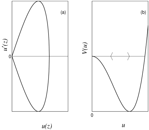
FIG. 2.: The schematic representation of the pulse solution in the anti-continuum limit.

It follows that it is possible to prepare the initial phases of all particles on this separatrix such that their uncorrelated motion resembles the motion of a pulse solution through the system. This solution is dynamically unstable because $V^{\prime\prime}(0)<0$.

Finally, we consider possible velocities for exponentially decaying pulses (11). We want to check whether our pulses can be subsonic ($s<s_{max}$) or supersonic ($s<s_{smax}$). Taking into account that [see Eq. (12)]

$$\gamma=C(\cosh\mu-1)-\frac{\mu^{2}s^{2}}{2}~{},$$ (19)

we compare $s$ with $s_{max}$. Defining $s_{0}=s_{max}=s$ we find that the pulse can be both subsonic and supersonic since in this case

$$s_{0}^{2}=C\frac{\cosh\mu+1-\sqrt{(\cosh\mu+1)^{2}-2(2+\mu^{2})}}{2+\mu^{2}}~{}$$ (20)

Consequently for fixed $C$ and $\mu$, $s$ has to be small enough to satisfy $C>C_{1}$ [see (13)], when $s(C_{1})>s_{0}$. Thus for $s_{0}<s<s(C_{1})$ the solutions are supersonic, while for $s<s_{0}$ they are subsonic.

Let us consider an explicit example of the sech-type profile. Suppose the profile is described by the function

$$u(z)=u_{0}\mbox{sech}(\mu z)$$ (21)

where $u_{0}$ is the amplitude of the pulse and $\mu$ its inverse width. Using the expressions

$$u^{\prime\prime}(z) = u_{0}\mu^{2}[\mbox{sech}(\mu z)-2\mbox{sech}^{3}(\mu z)]$$ (22)

$$= \mu^{2}\left[u(z)-2\frac{u^{3}(z)}{u_{0}^{2}}\right],$$ (23)

$$u(z-1)+u(z+1) = 2u_{0}\frac{\cosh(\mu z)}{\sinh^{2}\mu+\cosh^{2}(\mu z)}$$ (24)

$$= 2u_{0}^{2}\cosh\mu\frac{u(z)}{u_{0}^{2}+\sinh^{2}\mu~{}u^{2}(z)},$$ (25)

we reconstruct the on-site potential $V(u)$:

$$V(u) = -\frac{1}{2}[s^{2}\mu^{2}+2C]u^{2}+\frac{s^{2}\mu^{2}}{2u_{0}^{2}}u^{4}$$ (26)

$$+ Cu_{0}^{2}\frac{\cosh\mu}{\sinh^{2}\mu}\ln\left[\frac{u_{0}^{2}}{\sinh^{2}\mu}+u^{2}\right]~{}.$$ (27)

It is easy to check that its shape will change with $C$ exactly as described above. We can rewrite this potential in the following form:

$$V(u)=-\frac{1}{2}\kappa_{2}u^{2}+\frac{\kappa_{2}-2C}{2u_{0}^{2}}u^{4}+C\sqrt{a^{2}+u_{0}^{2}}\ln\left(a^{2}+u^{2}\right)$$ (28)

where the parameters of the solution $s$ and $\mu$ are given by

$$\mu=\mbox{arcsinh}(u_{0}/a)~{},~{}s=\frac{\sqrt{\kappa_{2}-2C}}{\mbox{arcsinh}(u_{0}/a)}~{}.$$ (29)

After proper rescaling constants $C$ and $u_{0}$ can be eliminated and, consequently, we can reduce the number of system parameters to two. However, we are not able to rewrite the potential $V(u)$ as a function independent from the parameters of the solution (21): $s,u_{0},\mu$. This means that we cannot answer so far whether the solution (21) comes as a family of solutions of (28) or is a unique solution of the obtained equations of motion.

B Moving kinks

Kinks or topological solitons are solutions which connect two minima of the on-site potential $V(u)$. If $V(u)$ has several equivalent minima, a countable infinite set of stationary (time-independent) kink solutions of the Klein-Gordon equation (4) exists (in contrast to the space-continuous case, where the continuum groups of translation symmetry provides a smooth family of stationary kink solutions). Some of these solutions will be local minima of the total energy, and some will correspond to saddles. The question whether moving kinks as TW solutions (7) exist is still open. Some results (see, e.g., [15]) suggest that kinks in discrete lattices experience a so-called Peierls-Nabarro barrier. One interpretation of this barrier is that it is the energy difference between stable stationary kinks and unstable stationary kinks. Indeed it is clear, that to unpin a stable stationary kink, one needs at least this amount of energy. Another more sophisticated approach - the collective coordinate approach - is a projection technique which aims at accounting for the dynamics of a kink-like object boosted to move along the lattice. By coupling the kinks center of mass coordinates to phonons, one arrives at the result that a moving kink will radiate, loose kinetic energy, and finally be trapped (pinned) by the lattice. Here the barrier appears as a height of maxima in a potential which is used to describe the kink motion.

Nevertheless, the analytical result of [13] suggests that it is possible to construct an exact moving kink solution. This result can be generalised for any profile $u(z)$ that satisfies the following conditions:

• $u(z\rightarrow\pm\infty)\rightarrow\pm u_{0}$

• $u(z)$ is monotonic in $]-\infty,+\infty[$

• $u(z)$ is analytic in $]-\infty,+\infty[$ .

Contrary to the case of pulse solutions, we do not need to require the function $u(z)$ to have certain symmetries, so that we can restrict ourselves to monotonicity only. A non-symmetric $u(z)$ profile will simply imply a non-symmetric function $V(u)$. If the above-mentioned conditions are satisfied, we again can uniquely map the function $u(z)$ onto the potential $V(u)$. For simplicity, we renormalise the variable $u(z)$ by the kink width $u(z)\rightarrow u(z)/u_{0}$.

If

$$u(z\rightarrow\pm\infty)\sim\pm\left(1-e^{-\mu|z|}\right)~{},$$ (30)

we can perform the asymptotic analysis similar to the case of the pulse solution. If $C<C_{1}$ [where $C_{1}$ comes from Eq. (13)] it follows $V^{\prime\prime}(\pm 1)<0$. Therefore the extremal points $u=\pm 1$ are maxima and, consequently, the asymptotic groundstates $u=\pm 1$ are unstable. The sign of $V^{\prime\prime}(\pm 1)$ changes at $C=C_{1}$ so that for $C>C_{1}$ these groundstates are stable. Another critical $C_{2}$ value is given by

$$C_{2}=\frac{s^{2}u^{\prime\prime\prime}(0)}{2[u^{\prime}(1)-u^{\prime}(0)]}~{}.$$ (31)

If $C<C_{2}$ the state $u=0$ is a minimum and if $C>C_{2}$ it is a maximum and we have the standard double-well potential. For details see Fig. 3.

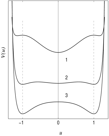
FIG. 3.: The potential $V(u)$ for a kink solution: 1: $C<C_{1}<C_{2}$, 2: $C_{1}<C<C_{2}$, and 3: $C_{1}<C_{2}<C$; The potential is obtained for positive $u$ values and continued to negative values for sake of transparency.

For

$$u(z)=\tanh(\mu z)$$ (32)

the explicit form of the potential $V(u)$ was obtained in [13] and [14] and can be written as follows

$$V(u) = (s^{2}\mu^{2}-C)u^{2}-\frac{s^{2}\mu^{2}}{2}u^{4}$$ (33)

$$- \frac{C}{\sinh^{2}\mu}\ln(\cosh^{2}\mu-u^{2}\sinh^{2}\mu)~{}.$$ (34)

The existence of such a solution does not imply the absence of Peierls-Nabarro barrier for stationary kink solutions. We demonstrate this for the particular case of the solution (32). We consider a chain with the on-site potential (34) with parameters $C=1$, $s=0.5$, $\mu=1$. Then we calculate two stationary kink solutions, one of which is stable, and the other one being a saddle in the energy landscape. Their energies are $E_{1}=0.991796$ and $E_{2}=0.992153$, respectively (measured relatively to the absolute energy minimum). The nonzero difference is the Peierls-Nabarro barrier. In fact, the existence of a Peierls-Nabarro barrier already follows from the stability of one of the stationary kink solutions, which implies that a finite amount of energy is needed to get out of the minimum.

Furthermore, we now are in possession of a very effective method to generate equations of motion which support stationary kinks without a Peierls-Nabarro potential, i.e., where a stationary kink exists which can be placed anywhere in the chain. Such a system has a degenerated ground state under the constraint of existence of one kink. It can be easily generated by putting $s=0$ in the above inverse method, and that is also true for pulse solutions. Indeed, in the limit $s\rightarrow 0$ we generate systems which support kinks (or pulses) which move with infinitesimally slow velocity. As the system is energy conserving and the kinetic energy becomes negligible in this limit, the groundstate becomes nearly degenerate, and a Goldstone mode appears for $s=0$. We tested these predictions numerically and obtained excellent agreement. A particular example of a potential supporting kinks with zero Peierls-Nabarro potential is

$$V(u)=-Cu^{2}-\frac{C}{\sinh^{2}\mu}\ln(\cosh^{2}\mu-u^{2}\sinh^{2}\mu)\;\;,$$ (35)

which was obtained for a kink solution $u(z)=\tanh(\mu z)$ from (34) by putting $s=0$. It is interesting to note that Ward and Speight [16] also proposed a scheme which generates systems supporting kink solutions with zero Peierls-Nabarro potential. This scheme uses Bogomolnyi’s inequality [17]. The structure of the potential functions was fixed, but the difference operators were chosen in an appropriate way. This method then generates equations of motion which are rather hard to justify physically. This is not the case when using our inverse method scheme.

C Reaction-diffusion systems

Let us also consider dissipative systems described by the discrete analogue of reaction-diffusion equation of the form

$$\dot{u}_{n}=C(u_{n+1}-2u_{n}+u_{n-1})+f(u_{n})~{}.$$ (36)

The physical background of this equation differs from the above considered nonlinear Klein-Gordon chains but it also admits localized travelling-wave solutions. These systems are dissipative because we have a first order time derivative instead of the inertia term. Here the function $f(u)$ can have different meanings, for example, an ion current for nerve fibers (see [18]).

These systems lack time reversibility. The equation for TW solutions reads

$$-su^{\prime}(z)=C[u(z+1)-2u(z)+u(z-1)]+f[u(z)]~{}.$$ (37)

To generate a system for a moving pulse, let us consider a symmetric pulse with one maximum as described in the pulse section of the Klein-Gordon chains. Due to the first order derivative in Eq. (37) the lhs is anti-symmetric, while the rhs is symmetric. Consequently, we cannot define $f(u)$ in a unique way. Any further complication of the symmetry of the pulse will not help either. Thus, we conclude that there exist no moving pulse solutions in Eq. (37).

However, reaction-diffusion systems (37) support kink solutions. The non-uniqueness problems disappear as long as the kink shape $u(z)$ is a monotonous function. Due to the first order derivative in Eq. (37) a kink shape moving to the right with some given velocity will generate a function $f_{r}$ different from the function $f_{l}$ generated by the same kink moving with the same velocity but to the left.

As an example, let us consider a profile $u(z)=\tanh(\mu z)$. Performing the above-mentioned computations we obtain

$$f(u)=-s\mu(1-u^{2})-2C\frac{u}{1+(1-u^{2})\sinh^{2}\mu}+2Cu$$ (38)

This result coincides with result of Bressloff and Rowlands (see [14]).

Finally, let us show that we can also obtain moving pulses provided we increase the number of components per site. Indeed consider

$$\dot{u}_{n} = C(u_{n+1}-2u_{n}+u_{n-1})+f(u_{n},v_{n})\;\;,$$ (39)

$$\dot{v}_{n} = C(v_{n+1}-2v_{n}+v_{n-1})+g(u_{n},v_{n})\;\;.$$ (40)

Assuming $u_{n}(t)=u(n-st)\;\;,\;\;v_{n}(t)=v(n-st)$ we find

$$-su^{\prime}(z)=C[u(z+1)-2u(z)+u(z-1)]+f[u(z),v(z)]\;\;,$$ (41)

$$-sv^{\prime}(z)=C[v(z+1)-2v(z)+v(z-1)]+g[u(z),v(z)]\;\;.$$ (42)

Let us choose a certain profile for $u(z)$. Fixing a value of $u=\kappa$ we obtain a countable set of points $z^{(u)}_{i}$ such that $u(z_{i})=\kappa$. Here $i$ is an integer and counts all points. This defines a countable set of functions $z^{(u)}_{i}(u)$. Similarly we proceed with $v(z)$. In order to solve the inverse problem, i.e., for given functions $u(z)$ and $v(z)$ we have only to require

$$v(z^{(u)}_{i})\neq v(z^{(u)}_{j})~{}~{}\mbox{if}~{}~{}i\neq j\;\;,\;\;u(z^{(v)}_{i})\neq u(z^{(v)}_{j})~{}~{}\mbox{if}~{}~{}i\neq j\;\;.$$ (43)

This is a weak condition satisfied by most choices of $u$ and $v$. For instance we can even choose symmetric functions having just one maximum and decaying to zero at infinities. The only restriction would be to shift the centers of the two functions apart, e.g., $v(z)=u(z-z_{0})$ for a given $u(z)$. But also asymmetric functions with even several maxima are allowed. Also possible is a symmetric function for $u(z)$ having one maximum and decaying at infinities, and an asymmetric function for $v(z)$ having the same other properties - with the maxima of both functions coinciding ($z_{0}=0$). It is a tedious work to calculate examples, so in most cases it will be appropriate to obtain the functions $f$ and $g$ numerically. The reason for the easy construction of two-component moving pulses is that we introduce two functions $f,g$ of two variables, but determine them only on a line in their phase space $\{u,v\}$. That means that we do not completely define these functions.

Adding a third component to the problem clearly further relaxes the conditions on the pulse forms. The existence of two component pulses is partially known for space continuous systems [19]. Note that our inverse method works as well in the space continuous case, i.e., where differences of the form $u_{n+1}-2u_{n}+u_{n-1}$ are replaced by second derivatives.

Why not doing the same for conservative systems? Then the functions $f,g$ will be the components of the gradient of some generating function (e.g., a potential). Thus, we have to impose this gradient condition, which will restrict the choice of functions $u,v$.

IV Acoustic chains

Now let us study systems which support acoustic (pulse) solitary waves. In these systems the on-site potential is absent [$V(u)=0$] and the solitary waves appear due to the nonlinearity of the interaction potential $W(r)$. First of all, we introduce the relative displacements, $r_{n}=u_{n+1}-u_{n}$. In these terms the equations of motion take the form

$$\ddot{r}_{n}=W^{\prime}(r_{n+1})-2W^{\prime}(r_{n})+W^{\prime}(r_{n-1}).$$ (44)

For TW solutions $r_{n}(t)=r(n-st)=r(z)$ one can write

$$W^{\prime}[r(z+1)]=s^{2}r^{\prime\prime}(z)+2W^{\prime}[r(z)]-W^{\prime}[r(z-1)].$$ (45)

As shown in [3], in such a lattice localized bell-shaped travelling-waves solutions can exist if $W(r)$ has a hard anharmonicity in the region $r<0$. Note that the acoustic solitons correspond to a localized contraction of the chain and therefore the function $r(z)$ should be completely negative.

It is evident by following the above line of argumentation for Klein-Gordon chains, that the pulse $r(z)$ has to be symmetric and must have only one maximum. Any deviation from this leads to a non-uniqueness in the definition of the potential. This implies that acoustic chains admit at the best moving kink solutions (non-topological) in the original variables $u_{n}(t)$, and even these kink solutions have to have reflection symmetry.

Suppose the function $r(z)$ satisfies the conditions for the pulses given in Subsec. IIIA. Then due to the symmetry of $r(z)$,

$$W^{\prime}(r_{1})=W^{\prime}(r_{0})+\frac{1}{2}s^{2}r^{\prime\prime}(0)$$ (46)

where $r_{0}=r(0)~{}$, $r_{1}=r(1)$. In order to find the unknown function $W^{\prime}(r)$ we have to solve the initial value problem (45) where the initial condition should be a the function $W^{\prime}(r)$ on the interval $r_{0}<r<r_{1}$. If $W^{\prime}(r)$ is defined on this interval, using Eqs. (45) and (46), one can construct the function $W^{\prime}(r)$ for $r>r_{1}$ which will be uniquely defined (see Fig. 4) for each $W^{\prime}(r)$. This means that we can choose $W^{\prime}(r)$ in $[r_{0},r_{1}]$ arbitrarily.

FIG. 4.: The schematic representation of the creation of the potential $W(r)$ for acoustic chains. Different initial value choices will generate different potentials for one and the same TW profile.

Therefore we find that for given $\{r(z),s\}$ a countable infinite dimension of the space of solutions $W(r)\in C^{2}$ exists. Each function from this set supports one and the same $r(z)$ as an exact solution with one and the same velocity. However, the function constructed in this way from an arbitrary initial value will be non-analytic in general (it is easy to show that all functions will be twice differentiable).

To avoid the problem of generating non-analytic potential functions, we found another way of constructing the potential. Suppose $r(z)$ is a pulse. Then $W^{\prime}[r(z)]\equiv\rho(z)$ is also a pulse. Let us rewrite Eq. (45) as

$$r^{\prime\prime}(z)=\frac{\rho(z+1)-2\rho(z)+\rho(z-1)}{s^{2}}~{}.$$ (47)

Now instead of defining $r(z)$ we define $\rho(z)$ (symmetric bell-shaped pulse). If this function is analytic, the rhs of Eq. (47) is also analytic. Then simply integrating this rhs twice, we find an analytic function $r(z)$ which is also of a bell-shaped form provided $\rho(z)$ decays for large $z$ faster than $1/z^{2}$. Having $r$ as a function of $\rho$ (on a half axis $z$) we can invert this dependence and consider $\rho$ as a function of $r$. This gives us the force function $W^{\prime}(r)$. Notice that by that we can avoid generating non-analytic potentials.

Finally, let us take a look at the asymptotic behavior of the solitary solution. Suppose $\rho(z)\sim e^{-\mu z}$ for $z\rightarrow\infty$ and $W^{\prime}(r)\simeq Cr$ for $r\rightarrow 0$. Linearising Eq. (6), we obtain

$$\frac{s^{2}}{C}=2\frac{\cosh\mu-1}{\mu^{2}}>1~{}.$$ (48)

Thus, each moving acoustic soliton is supersonic.

In the following example we will illustrate how to construct the interaction potential from a given solution profile. Suppose $\rho(z)=\rho_{0}~{}\mbox{sech}^{4}(\mu z)$. We substitute it into the rhs of Eq. (47) and integrate it twice. Using the formula

$$\int\int\mbox{sech}^{4}(\mu z)dzdz=-\frac{1}{6\mu^{2}\cosh^{2}(\mu z)}$$ (49)

$$+\frac{2}{3\mu^{2}}\ln[\cosh(\mu z)]+K_{1}z+K_{2}~{}$$ (50)

we calculate the function $r(z)$. In order to satisfy the boundary conditions, we put $K_{1}=0$, $K_{2}=0$. As a result, we obtain

$$r(z)=\frac{\rho_{0}}{3s^{2}\mu^{2}}\left[\ln\xi(z)+\sqrt{\rho(z)\over\rho_{0}}\left(1-\frac{2(\sinh^{2}\mu-1)-\xi(z)}{\xi^{2}(z)}\right)\right]~{},~{}\xi(z)=1+\sqrt{\frac{\rho(z)}{\rho_{0}}}\sinh^{2}\mu~{}.$$ (51)

We cannot express the force function $W^{\prime}(r)$ explicitly from the above formula, but we have the inverse relation $r(z)=D[\rho(z)]$ where D is a function inverse to $W^{\prime}$. The potential $W(r)$ can be calculated numerically.

V Breathers of the DNLS-type equations

Here we study a general nonlinear chain governed by Eq. (3). It is already known that these systems have standing breather solutions (see, e.g., [20]). The standing breather is defined as a spatially localized solution which is periodic in time. The general breather solution with frequency $\omega$, velocity $s$ and wavenumber $q$ can be chosen to be

$$\phi_{n}(t)=\Phi(n-st,\Omega t)\;\;,\;\;\Phi(x\rightarrow\pm\infty,y)\rightarrow 0\;\;,\;\;$$ (52)

$$\Phi(x,y)=\Phi(x,y+2\pi)\;\;.$$ (53)

Periodicity of $\Phi(x,y)$ in $y$ allows to expand it into a Fourier series:

$$\Phi(x,y)=\sum_{k}\Phi_{k}(x){\rm e}^{ik\Omega t}\;\;.$$ (54)

For DNLS systems these solutions may have only one nonzero Fourier harmonic w.r.t. time. Since the DNLS equation has a gauge symmetry $\phi_{n}(t)\rightarrow e^{i\omega t}\psi_{n}(t)$, we can actually always transform a breather solution into a stationary pulse solution (note that this is not possible for breather solutions of e.g., Klein-Gordon or acoustic chains). As a result Eq. (3) can be rewritten as

$$i{\dot{\psi}}_{n} + \kappa\psi_{n}+C(\psi_{n+1}+\psi_{n-1})+F(|\psi_{n}|^{2})(\psi_{n-1}+\psi_{n+1})$$ (55)

$$+ G(|\psi_{n}|^{2})\psi_{n}=0~{}$$ (56)

where $\kappa=-\omega-2C$. Then we can define $\psi_{n}(t)=R(z)+iI(z)~{}$, $z=n-st~{}$, where the functions $R$ and $I$ are real. Separating real and imaginary parts of Eq. (56) we obtain the unknown nonlinear functions $F$ and $G$ expressed in terms of breather envelope $R$ and $I$ and breather parameters

$$F[R^{2}(z)+I^{2}(z)] = -C+\frac{[R^{2}(z)+I^{2}(z)]^{\prime}}{2\left(R(z)[I(z-1)+I(z+1)]-I(z)[R(z-1)+R(z+1)]\right)}~{},$$ (57)

$$G[R^{2}(z)+I^{2}(z)] = -\kappa-\frac{s}{R(z)}\left[I^{\prime}(z)-\frac{[R^{2}(z)+I^{2}(z)]^{\prime}}{2\left(I(z)-\frac{I(z-1)+I(z+1)}{R(z-1)+R(z+1)}R(z)\right)}\right]~{}.$$ (58)

We are interested in symmetric profiles, i.e., $u(z)\equiv\sqrt{R^{2}(z)+I^{2}(z)}=u(-z)$ in order to ensure single value properties of the functions $F,G$. It is easy see that the profile is symmetric and bell-shaped if, e.g., both $I(z)$ and $R(z)$ are symmetric or one of these functions is symmetric and another one is anti-symmetric. The lhs of Eq. (58) is symmetric. If $R$ and $I$ are symmetric, the functions $R(z-1)+R(z+1)$ and $I(z-1)+I(z+1)$ are also symmetric and the derivative of $R^{2}(z)+I^{2}(z)$ is anti-symmetric. Consequently, the rhs of this equation is anti-symmetric. Obviously, this is possible only for a trivial solution $\psi_{n}(t)=0$.

Clearly moving solutions seem to have more complicated internal structures, as known from the solutions of the Ablowitz-Ladik system [12]. These solutions can be represented in the following form:

$$\phi_{n}(t)=u_{n}(t)e^{i(qn-\omega t)}=u(z)e^{i(qn-\omega t)}~{},~{}~{}z=n-st~{}$$ (59)

where $u(z)$ is a real envelope amplitude, $s$ is breather velocity, $q$ its wave number and $\omega$ its frequency. Substituting this ansatz into Eq. (3), we obtain two equations for real and complex parts:

$$(\omega-2C)u(z) + \cos{q}(C+F[u^{2}(z)])[u(z-1)+u(z+1)]+G[u^{2}(z)]u(z)=0~{},$$ (60)

$$-su^{\prime}(z) + \sin{q}(C+F[u^{2}(z)])[u(z+1)-u(z-1)]=0~{}.$$ (61)

After straightforward calculations the unknown nonlinear functions $F$ and $G$ can be expressed in terms of $u$ and the system parameters:

$$F[u^{2}(z)] = -C-\frac{s}{\sin{q}}\cdot\frac{u^{\prime}(z)}{u(z+1)-u(z-1)}~{},$$ (62)

$$G[u^{2}(z)] = -(\omega-2C)-\cos{q}(C+F[u^{2}(z)])\frac{u(z-1)+u(z+1)}{u(z)}$$ (63)

$$= -(\omega-2C)-\frac{s}{\tan{q}}\cdot\frac{u^{\prime}(z)}{u(z)}\cdot\frac{u(z-1)+u(z+1)}{u(z+1)-u(z-1)}.$$ (64)

If the envelope function $u(z)$ satisfies the conditions

• $u(z\rightarrow\pm\infty)\rightarrow 0$

• $u(-z)=u(z)$

• $u(z)$ is monotonic in $[0,+\infty[$

• $u(z)$ is analytic in $[0,+\infty[$,

we can postulate again (similarly to Sections III and IV) that for any envelope $u(z)$ defined as above and the set of parameters ($s,q,\omega$) one can uniquely define the nonlinearity for the equation given by functions $F$ and $G$.

A Examples

Let us consider the particular case when $u(z)=u_{0}\mbox{sech}^{2}(\mu z)$. Substituting this expression into Eqs. (62) and (64), we obtain functions $F$ and $G$:

$$F(u^{2}) = -C+\frac{s\mu}{\sin q~{}\sinh 2\mu}\left[1+\frac{\sinh^{2}\mu}{u_{0}}u\right]^{2}~{},$$ (65)

$$G(u^{2}) = -(\omega-2C)-\frac{2s\mu}{\tan q~{}\sinh 2\mu}$$ (66)

$$\times \left(\cosh{2\mu}-\frac{\sinh^{2}\mu}{u_{0}}u\right)~{}.$$ (67)

1 The Ablowitz-Ladik equation

Let us look at the particular case when $G\equiv 0$. In this case we have only one unknown nonlinear function, $F$. After simplifying the ansatz (62)-(64) we obtain

$$\frac{u^{\prime}(z)}{u(z)} = -\frac{(2C-\omega)\tan{q}}{s}\cdot\frac{u(z+1)-u(z-1)}{u(z-1)+u(z+1)}~{},$$ (68)

$$F[u^{2}(z)] = -C+\frac{(2C-\omega)u(z)}{\cos q[u(z-1)+u(z+1)]}.$$ (69)

In the particular case $u(z)=u_{0}\mbox{sech}(\mu z)$ we obtain the quadratic function

$$F(u^{2})=-C+\frac{2C-\omega}{2\cos q~{}\cosh\mu}\left[1+\frac{\sinh^{2}\mu}{u_{0}^{2}}u^{2}\right]~{}.$$ (70)

We assume

$$\frac{2C-\omega}{2\cos q~{}\cosh\mu}=C~{},~{}~{}\frac{2C-\omega}{2\cos q~{}\cosh\mu}\cdot\frac{\sinh^{2}\mu}{u_{0}^{2}}=\frac{\lambda}{2}~{},~{}~{}\lambda>0~{}.$$ (71)

Eq. (68) yields

$$2C-\omega=\frac{s\mu}{\tan q~{}\tanh\mu}~{}.$$ (72)

We can rewrite these equations in more common way, expressing the parameters of the solution $s,\omega$ and $u_{0}$ through $q$ and $\mu$:

$$u_{0}=\sqrt{\frac{2C}{\lambda}}\sinh\mu~{},~{}\omega=2C[1-\cosh\mu~{}\cos q]~{},~{}s=2C\frac{\sinh\mu}{\mu}\sin q~{}.$$ (73)

This corresponds to the well-known integrable Ablowitz-Ladik equation.

2 DNLS with local nonlinearity

Now let us look at a well-known equation of the DNLS family. In the case of $F(u^{2})\equiv 0$, we have

$$i\dot{\phi}_{n}+C(\phi_{n+1}-2\phi_{n}+\phi_{n-1})+G\left(|\phi_{n}|^{2}\right)\phi_{n}=0~{}.$$ (74)

We substitute the ansatz (59) and consider Eq. (60) that for this particular case takes the following form:

$$u^{\prime}(z)=\alpha[u(z+1)-u(z-1)]~{},~{}~{}\alpha=\frac{C\sin q}{s}~{}.$$ (75)

The absence of a to be defined function in this equation, contrary to the previous examples, makes this equation an equation for the pulse shape. Let us show that a pulse shaped function $u(z)$ can not satisfy Eq. (75). Suppose first that our solution $u(z)$ is periodic with some large period $L$. In this case we can expand the solution into Fourier series

$$u(z)=\sum_{m=-\infty}^{+\infty}u_{m}\exp{\left(im\frac{2\pi}{L}z\right)}~{}.$$ (76)

Substituting this expansion into Eq. (75) we obtain the algebraic equation

$$m\frac{2\pi}{L}=2\alpha\sin\left(m\frac{2\pi}{L}\right)$$ (77)

where $m$ is unknown integer. The equation $x=2\alpha\sin{x}$ always has always a finite number of roots for any non-zero $\alpha$. Since $m$ is integer, we can actually solve (77) only for some specific values of $\alpha$. This does not depend on $L$, so we can consider the limit $L\rightarrow\infty$. A pulse solution $u(z)$ would require an infinite number of nonzero harmonics in Eq. (76). Therefore it is impossible to satisfy Eq. (75) with a pulse shaped $u(z)$. Consequently, Eq. (74) does not admit moving breathers.

It appears to be not possible to extend this method to systems like acoustic or KG chains. Note, that the spectrum of a DNLS-breather consists only of one frequency and therefore can be transformed into two differential delay/advance equations while acoustic/KG breathers will have an infinite number of harmonics and obviously cannot be rewritten as a countable number of retarded and advanced ODE’s.

VI Continuation of moving solutions for conservative systems

Let us discuss the question, whether a conservative system which allows for a certain moving solution and has been generated by our inverse method, has this solution as an isolated one, or as a part of a smooth family of solutions. In other words, we consider a given moving solution, generate the equations of motion, and search in the phase space vicinity of our solution for other moving solutions. That calls for a linear stability analysis of the phase space flow around the given moving solution. Since our solution has some uniform asymptotic ground state (we assume that the parameters are such that the uniform asymptotic state is a ground state, see discussions above), we know that a part of the linear stability analysis spectrum will be given by just solving the eigenvalue problem of linearized fluctuations around the ground state. The eigenvectors will be plane waves ${\rm e}^{i(qn-\omega_{q}t)}$ (they will be deformed in the center of our moving solution) and their spectrum is given by some dispersion relation $\omega_{q}$. Note that due to space discreteness $\omega_{q}$ is periodic in $q$. Let us search for $q$ values for which the plane wave can be cast into the form

$${\rm e}^{i(qn-\omega_{q}t)}=h_{q}(n-st)\;\;.$$ (78)

This is possible if

$$qs=\omega_{q}\;\;.$$ (79)

Consider first the case of an acoustic chain. For small $q$ we have $\omega_{q}=vq$ with $v<s$ (because all moving solutions will be supersonic, see discussions above). Consequently, there is only the trivial solution $q=0$ of Eq. (79), which simply corresponds to a shift of the center of mass of the acoustic chain. We can always work in the frame where the center of mass is resting at zero. Consequently, for acoustic chains we do not find plane waves which move with the same velocity as the original solution. That implies that there are no small perturbations of our solution which have plane wave asymptotics and yield again a moving solution. Thus, we conclude that if moving solutions are coming in families, all solutions on the family will be localized in space.

Consider now the case of an optical chain (KG case). Since $\omega_{q=0}\neq 0$, we will always find at least one nonzero $q$-value (in general it will be a finite number of $q$ values which tends to infinity as $s\rightarrow 0$) which solves Eq. (79). In that case we do know that there will exist perturbations with plane wave asymptotics which deform our original localized moving solution into a partly delocalized one, which is now in addition characterized by a nonzero amplitude in the asymptotics (i.e., the kink has oscillating tails at $|z|\rightarrow\infty$). Some numerical results that confirm the above-mentioned arguments are given in [21].

To further analyse this, we performed a numerical continuation of a moving solution using the pseudo-spectral method which is essentially a Newton method in $q$ space (see, e.g., [22],[23]). We chose the moving kink solution (32) which yields the potential (34). The numerical method traces the phase space of the system for moving solutions nearby the starting one with slightly changed velocities and shapes.

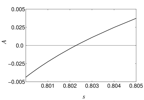
FIG. 5.: Dependence of the amplitude in the asymptotics of a moving kink on the velocity for a given equation (see text).

In Fig. 5 we show the dependence of the amplitude $A$ of the asymptotics versus velocity $s$. We indeed find that our chosen solution (32) (with $C=1$, $\mu=\ln{(1+\sqrt{2})}$, $s=1/[\sqrt{2}\ln{(1+\sqrt{2})}]\simeq 0.802278$ in this particular case) can be continued, but it thus gets dressed with plane wave asymptotics. The change of sign in the amplitude implies a phase change from $0$ to $\pi$. A slightly changed potential will exhibit similar solutions but with slightly shifted curves in Fig. 5 . Thus, it follows that the moving solution with uniform asymptotics is structurally stable, i.e., has a similar solution with uniform asymptotics for slightly changed equations of motion. This follows from the fact that the crossing of the $A(s)$ curve in Fig. 5 with $A=0$ is a generic intersection.

VII Moving pulses in higher lattice dimensions

So far we have been discussing moving pulses and kinks in one-dimensional lattices. In this chapter we will show that the inverse method can be easily generalized to higher space dimensions for reaction-diffusion equations, provided we take into account two or more components.

Let us consider a two-dimensional lattice. The function $u_{n}(t)$ will now depend on two lattice indices $u_{m,n}(t)$. The differences $(u_{n-1}+u_{n+1}-2u_{n})$ will now turn into some general discrete Laplacians $D(u_{m,n})$. Assuming a moving solution in the form

$$u_{m,n}(t)=u(m-s_{x}t,n-s_{y}t)\equiv u(x,y)$$ (80)

we arrive at the equations

$$-s_{x}u_{,x}-s_{y}u_{,y}+D[u(x,y)]=f(u)\;\;.$$ (81)

Fixing a value of $u$ we obtain a line in the $\{x,y\}$ space and since the rhs should not change, the lhs should be constant on this line - a very restrictive condition. If we instead consider two components moving in the same directions with same velocities, the equations become

$$-s_{x}u_{,x}-s_{y}u_{,y}+D[u(x,y)]=f(u,v)\;\;,$$ (82)

$$-s_{x}v_{,x}-s_{y}v_{,y}+D[v(x,y)]=g(u,v)\;\;.$$ (83)

Again fixing a value for $u$ we obtain some line in $\{x,y\}$. If we consider a functions $u,v$ decaying to zero at infinities, this line will be a closed loop. Let us assume that $v$ is not constant on the loops of constant $u$. That helps, but still if we fix some point on the loop with some given value of $v$ there will be a countable number of other points $p_{i}$ on the loop where $v$ takes the same value. Then the lhs’s of Eqs. (82) and (83) have to be equal in these points. We can satisfy this condition by demanding two symmetries but only in the case when we have only two points $p_{i}$. First our pulse functions $u,v$ should be invariant under reflections at a line parallel to the direction of motion. This ensures that the first order derivatives on the lhs’s of Eqs. (82) and (83) will be the same in all $p_{i}$. To ensure invariance of the Laplacians in $p_{i}$ we only have to demand that the chosen direction of motion (defined by $s_{x},s_{y}$) is parallel to a reflection symmetry line of the lattice. For instance, for a square lattice these will be only the major lattice axes and the diagonals. The initially assumed condition that $v$ varies along the loop of constant $u$ can be, e.g., easily satisfied by considering pulses which are symmetric under point reflections and whose symmetry centers are shifted along the line of motion. Note that contrary to the one-dimensional case the inverse method yields the functions $f,g$ in a two-dimensional part of their phase space $\{u,v\}$.

What if we add a third component? The conditions weaken again, similarly to the case of two components in the one-dimensional lattice. For instance, one can design pulses where two components are invariant under point reflections with centers shifted along the line of motion, and the third component will be off-centered from the line connecting the two first centers.

Let us consider a three-dimensional lattice and two components. Fixing $u$ we now obtain a closed surface in $\{x,y,z\}$. Requiring $v$ to generally vary on this surface, we find that $v$ will stay constant at least on loops embedded on the surface. Since the lattice is invariant only under discrete symmetries, we can not satisfy invariance of the lhs’s of equations similar to Eqs. (82) and (83) on this loop. Consequently, there exist no moving two-component pulses in a three-dimensional lattice (and straightforwardly in any higher-dimensional lattice). This is in contrast to the space-continuous case, where space is invariant under continuous symmetries. Then we can satisfy the invariance of the lhs’s along the loop trivially if both pulses are invariant under rotations around a line pointing in the direction of their motion. The initial condition that $v$ is constant only on loops (not on the whole surface) is easily obtained by considering pulses $u,v$ with shifted centers, just as in the two-dimensional case.

Adding a third component $w$ to the three-dimensional lattice case reduces the problem of constant $v$ and $w$ on a loop to that in a countable set of points $p_{i}$. Still we need a symmetry to ensure invariance of lhs’s in the points $p_{i}$. This is easily achieved in the case when we have only two points $p_{i}$ by demanding two symmetries. First we need all three components $u,v,w$ to be invariant under reflection at a plane which contains the direction of motion. Secondly this plane has to be parallel to any mirror reflection symmetry plane of the lattice. Again the initial condition of having just countable sets of points $p_{i}$ with coinciding values $\{u,v,w\}$ can be achieved by shifting the centers of the three pulse components apart while staying on one line - the direction of motion. For instance, for a cubic lattice with lattice points at $x=l,y=m,z=n$ and $l,m,n$ integer reflection symmetry planes are $\{x,y,0\}$, $\{0,y,z\}$, $\{x,0,z\}$, $\{x,\pm x,z\}$, $\{x,\pm z,z\}$, $\{x,y,\pm x\}$ among possible others. Any vector embedded in these planes is an allowed moving direction.

VIII Conclusions

In this paper we have studied several types of nonlinear lattice systems. Contrary to most of papers on nonlinear lattices where authors try to find a solution (either analytically or numerically) of the given system, we approach the problem from the opposite side - we look for the system (in fact, for the interaction and/or on-site potentials) which admits some specific solution.

We have studied kinks and pulses in the Klein-Gordon system, acoustic solitons in chains with nonlinear intersite interactions and discrete breathers in the nonlinear Schrödinger-type systems. In all these cases the method enables us to generate a unique on-site or interaction potential for a given pulse or kink and its velocity if this solution satisfies certain conditions. As a particular result, we have shown that the acoustic solitons are always supersonic. We also conclude that nonzero Peierls-Nabarro barrier does not prevent discrete kinks from propagating with constant velocities. In the case of discrete moving breathers in DNLS-type systems we create nonlinear terms in the equation (3) for given envelope profile and breather frequency, wave number and velocity.

Our method is equally well suited for dissipative systems. Systems of coupled reaction-diffusion equations do not possess one important property which is time reversibility and therefore despite being closely related to the Klein-Gordon type equations, do not have pulse travelling-wave solutions in the one-dimensional case for one component. We generalize the search for pulses to higher lattice dimensions and find that moving pulses can be easily obtained provided we also increase the number of components.

All presented results can be easily extended to systems with longer range interactions, and to space continuous systems (i.e., to partial differential equations). Note that the continuum limit of the considered difference equations is easily recovered by choosing solitary wave profiles which vary slowly along the lattice.

- [1] M. Toda, Theory of Nonlinear Lattices (Springer Verlag, Berlin, 1989).
- [2] J. K. Hale and S. M. V. Lunel, Introduction to Functional Differential Equations (Springer Verlag, Berlin, 1993).
- [3] G. Friesecke and J. A. D. Wattis, Commun. Math. Phys. 161, 391 (1994).
- [4] S. J. Orfanidis, Phys. Rev. D 18, 3823 (1978).
- [5] S. Flach and C. R. Willis, Phys. Rep. 295, 181 (1998).
- [6] K. Hori and S. Takeno, J. Phys. Soc. Japan 61, 2186 (1992).
- [7] C. Claude, Y. S. Kivshar, O. Kluth, and K. H. Spatschek, Phys. Rev. B 47, 14228 (1993).
- [8] S. Flach and C. R. Willis, Phys. Rev. Lett. 72, 1777 (1994).
- [9] D. Chen, S. Aubry, and G. P. Tsironis, Phys. Rev. Lett. 77, 4776 (1996).
- [10] S. Aubry and T. Cretegny, Physica D 119, 34 (1998).
- [11] S. Flach and K. Kladko, Physica D in print (1998).
- [12] M. J. Ablowitz and J. F. Ladik, J. Math. Phys. 17, 1011 (1976).
- [13] V. H. Schmidt, Phys. Rev. B 20, 4397 (1979).
- [14] P. C. Bressloff and G. Rowlands, Physica D 106, 225 (1997).
- [15] M. Peyrard and M. D. Kruskal, Physica D 14, 88 (1984).
- [16] J. M. Speight and R. S. Ward, Nonlinearity 7, 475 (1994).
- [17] E. B. Bogomol’nyi, Sov. J. Nucl. Phys. 24, 449 (1976).
- [18] A. C. Scott, Rev. Mod. Phys. 47, 487 (1975).
- [19] A. S. Michailov, Foundations of Synergetics I (Springer Verlag, Berlin, 1994).
- [20] R. S. MacKay and S. Aubry, Nonlinearity 7, 1623 (1994).
- [21] A. V. Savin, Y. Zolotaryuk, and J. C. Eilbeck, submitted to Physica D (1999).
- [22] J. C. Eilbeck and R. Flesch, Phys. Lett. A 149, 200 (1990).
- [23] Y. Zolotaryuk, J. C. Eilbeck, and A. V. Savin, Physica D 108, 81 (1997).