On the degenerated soft–mode instability

Abstract

We consider instabilities of a single mode with finite wavenumber in inversion symmetric spatially one dimensional systems, where the character of the bifurcation changes from sub– to supercritical behaviour. Starting from a general equation of motion the full amplitude equation is derived systematically and formulas for the dependence of the coefficients on the system parameters are obtained. We emphasise the importance of nonlinear derivative terms in the amplitude equation for the behaviour in the vicinity of the bifurcation point. Especially the numerical values of the corresponding coefficients determine the region of coexistence between the stable trivial solution and stable spatially periodic patterns. Our approach clearly shows that similar considerations fail for the case of oscillatory instabilities.

1 Introduction

Pattern formation in systems of large size has attracted much research interest in recent years. Especially the fact that many aspects, at least of one–dimensional systems or of quasi one–dimensional patterns, can be described by reduced equations of motion has allowed for linking quite different fields of physics (cf. [1] and references therein). To some extent the approach strongly parallels the normal form calculations in low dimensional dynamical systems [2], The reduced equations for simple instabilities, i. e. the Ginzburg–Landau equation is well established and its derivation can even be found in textbooks [3]. However, at least from the general point of view, less is known if additional constraints are imposed on the instability, that means if higher order codimension bifurcations are considered.

We are here concerned with instabilities in spatially one dimensional systems where a single mode becomes unstable with respect to a wavenumber $q_{c}$ due to an eigenvalue zero in the spectrum. Such a situation occurs generically in inversion symmetric situations and we henceforth consider such systems. Let $\lambda(k,\underline{\mu})$ denote the corresponding critical eigenvalue in dependence on the wavenumber $k$ and the system parameters $\underline{\mu}$. It obeys

$$\lambda(q_{c},\underline{\mu})=0,\quad\left.\partial_{k}\lambda(k,\underline{\mu})\right|_{k=q_{c}}=0,\quad\left.\partial^{2}_{k}\lambda(k,\underline{\mu})\quad\right|_{k=q_{c}}<0\quad.$$ (1)

These conditions trace a codimension one set, i. e. a hypersurface in the parameter space on which the instability occurs. It is well established, even from a rigorous point of view [4], that the dynamics near such an instability is governed by a slowly varying envelope which obeys a real Ginzburg–Landau equation. Whether the instability is sub– or supercritical, i. e. whether the amplitude saturates in the vicinity of the instability, depends on the sign of the cubic term. The transition from sub– to supercriticality, i. e. the change of the sign, leads to a codimension two bifurcation. It is of course contained in the bifurcation set determined by eqs.(1). Such instabilities, which for example are relevant in the hydrodynamic context (cf. [5] for a recent reference) are at the centre of interest of our contribution.

From pure symmetry considerations the structure of the reduced amplitude equation may be fixed, taking the translation and inversion symmetry into account

$$\partial_{\tau}\bar{A}=\bar{\eta}\bar{A}+D\partial^{2}_{\xi}\bar{A}+\bar{r}|\bar{A}|^{2}\bar{A}+s|\bar{A}|^{4}\bar{A}+{\mathrm{i}}g|\bar{A}|^{2}\partial_{\xi}\bar{A}+{\mathrm{i}}d\bar{A}^{2}\partial_{\xi}\bar{A}^{*}\quad.$$ (2)

However, these considerations do not tell us whether such an equation is valid at all, and how the coefficients depend on the actual parameters of the underlying equations of motion. We present the complete derivation of the amplitude equation (2) starting from a general equation of motion, even if the method is in principle well established in the hydrodynamic context. But our approach is purely algebraic and has the advantage, that the results can be applied immediately to quite different physical situations. As a by–product we remark that for the similar hard–mode case a comparable approach fails, in contrast to statements in the literature. Finally we will dwell on some properties of eq.(2), since a complete discussion is difficult to find in the literature, despite the fact that related results from different points of view can be found quite frequently [6, 7, 8, 9].

2 Derivation of the amplitude equation

2.1 Notation

We suppose that the basic equation of motion for the $N$–component real field $\underline{\Phi}(x,t)$ is cast into the form

$$\partial_{t}\underline{\Phi}={\cal L}_{\underline{\mu}}\underline{\Phi}+{\cal N}[\underline{\Phi};\underline{\mu}]$$ (3)

such that the trivial translation invariant stationary state is given by $\underline{\Phi}\equiv 0$ . For the linear operator, which determines the instability of this state, we allow for an expression as general as possible, i. e.

$${\cal L}_{\underline{\mu}}\underline{\Psi}=\sum_{\alpha}\underline{\underline{L}}_{\alpha}(\underline{\mu})\partial^{\alpha}_{x}\underline{\Psi}\quad.$$ (4)

Using plane wave solutions $\underline{u}\exp({\mathrm{i}}kx)$ the eigenvalue problem is completely determined by the $N\times N$ matrices

$$\underline{\underline{L}}(k;\underline{\mu})=\sum_{\alpha}\underline{\underline{L}}_{\alpha}(\underline{\mu})({\mathrm{i}}k)^{\alpha}$$ (5)

according to

$$\underline{\underline{L}}(k;\underline{\mu})\underline{u}_{k}(\underline{\mu})=\lambda(k,\underline{\mu})\underline{u}_{k}(\underline{\mu})\quad.$$ (6)

We denote by $\lambda$ the eigenvalue branch with maximal real part, which obeys eqs.(1) at the instability. In our case the inversion symmetry guarantees that all quantities are real valued.

For the nonlinear part we employ an expansion in powers of the field according to

$${\cal N}(\underline{\Psi};\underline{\mu})={\cal N}_{2}(\underline{\Psi};\underline{\mu})+{\cal N}_{3}(\underline{\Psi};\underline{\mu})+{\cal N}_{4}(\underline{\Psi};\underline{\mu})+{\cal N}_{5}(\underline{\Psi};\underline{\mu})+\cdots$$ (7)

where

$${\cal N}_{2}(\underline{\Psi};\underline{\mu})=\sum_{\alpha,\beta}\underline{C}^{(\alpha\beta)}_{\underline{\mu}}\{\partial^{\alpha}_{x}\underline{\Psi},\partial^{\beta}_{x}\underline{\Psi}\}$$ (8)

$${\cal N}_{3}(\underline{\Psi};\underline{\mu})=\sum_{\alpha,\beta,\gamma}\underline{D}^{(\alpha\beta\gamma)}_{\underline{\mu}}\{\partial^{\alpha}_{x}\underline{\Psi},\partial^{\beta}_{x}\underline{\Psi},\partial^{\gamma}_{x}\underline{\Psi}\}$$ (9)

denote the most general expressions of second and third order, with vector valued bi– and trilinearforms $\underline{C}^{(\alpha\beta)}$ and $\underline{D}^{(\alpha\beta\gamma)}$. Written in components they read for example

$$\left(\underline{C}^{(\alpha\beta)}_{\underline{\mu}}\{\underline{u},\underline{v}\}\right)_{m}=\sum_{k,l}c_{\underline{\mu};mkl}^{(\alpha\beta)}u_{k}v_{l}\quad.$$ (10)

The contributions of order four and five are understood in the same way using the notation $\underline{E}^{(\alpha\beta\gamma\delta)}$ and $\underline{F}^{(\alpha\beta\gamma\delta\epsilon)}$ for the corresponding multilinearforms. In the subsequent analysis it is necessary to evaluate the nonlinearities if plane waves are inserted for the field. To be specific only waves with the multiples of the critical wavenumber $q_{c}$ will occur. In such a case all the nonlinearities are expressed in terms of the abbreviations (cf. eq.(5))

$$\underline{C}_{mn}(\underline{u},\underline{v};\underline{\mu}):=\sum_{\alpha\beta}({\mathrm{i}}mq_{c})^{\alpha}({\mathrm{i}}nq_{c})^{\beta}\underline{C}^{(\alpha\beta)}_{\underline{\mu}}\{\underline{u},\underline{v}\}$$ (11)

$$\underline{D}_{lmn}(\underline{u},\underline{v},\underline{w};\underline{\mu}):=\sum_{\alpha\beta\gamma}({\mathrm{i}}lq_{c})^{\alpha}({\mathrm{i}}mq_{c})^{\beta}({\mathrm{i}}nq_{c})^{\gamma}\underline{D}^{(\alpha\beta\gamma)}_{\underline{\mu}}\{\underline{u},\underline{v},\underline{w}\}$$ (12)

$$\underline{E}_{klmn}(\underline{u},\underline{v},\underline{w},\underline{x};\underline{\mu}):=\sum_{\alpha\beta\gamma\delta}({\mathrm{i}}kq_{c})^{\alpha}({\mathrm{i}}lq_{c})^{\beta}({\mathrm{i}}mq_{c})^{\gamma}({\mathrm{i}}nq_{c})^{\delta}\underline{E}^{(\alpha\beta\gamma\delta)}_{\underline{\mu}}\{\underline{u},\underline{v},\underline{w},\underline{x}\}$$ (13)

$$\underline{F}_{jklmn}(\underline{u},\underline{v},\underline{w},\underline{x},\underline{y};\underline{\mu}):=\sum_{\alpha\beta\gamma\delta\epsilon}({\mathrm{i}}jq_{c})^{\alpha}({\mathrm{i}}kq_{c})^{\beta}({\mathrm{i}}lq_{c})^{\gamma}({\mathrm{i}}mq_{c})^{\delta}({\mathrm{i}}nq_{c})^{\epsilon}\underline{F}^{(\alpha\beta\gamma\delta\epsilon)}_{\underline{\mu}}\{\underline{u},\underline{v},\underline{w},\underline{x},\underline{y}\}$$ (14)

which are frequently used in what follows.

2.2 Weakly nonlinear analysis

Suppose that at $\underline{\mu}=\underline{\mu}_{c}$ a degenerated soft–mode instability occurs. Let $\underline{u}_{c}\exp({\mathrm{i}}q_{c}x)$ denote the marginally stable mode, i. e. $\underline{u}_{c}=\underline{u}_{q_{c}}(\underline{\mu}_{c})$ is the nulleigenvector of the matrix (5) at $\underline{\mu}=\underline{\mu}_{c}$ and $k=q_{c}$. In the vicinity of this parameter value, i. e. for

$$\underline{\mu}=\underline{\mu}_{c}+\varepsilon\underline{\mu}^{(1)}+\varepsilon^{2}\underline{\mu}^{(2)}+\cdots$$ (15)

the solution of the full equation is expanded as

$$\underline{\Phi}(x,t)=\varepsilon^{1/2}\underline{\Phi}_{1}+\varepsilon\underline{\Phi}_{2}+\varepsilon^{3/2}\underline{\Phi}_{3}+\varepsilon^{2}\underline{\Phi}_{4}+\varepsilon^{5/2}\underline{\Phi}_{5}+\cdots$$ (16)

$$\underline{\Phi}_{1}=\underline{u}_{c}\exp({\mathrm{i}}q_{c}x)A(\tau_{1},\tau_{2},\ldots,\xi_{1},\xi_{2},\ldots)+c.c$$ (17)

where $\varepsilon$ denotes a dimensionless smallness parameter. As usual the dynamics of the complex valued amplitude $A$, which possesses a slowly varying space–time dependence on the scales $\tau_{k}=\varepsilon^{k}t$, $\xi_{k}=\varepsilon^{k}x$, will be determined by the secular conditions of the expansion. However, before we proceed let us comment on the choice of the expansion. The actual expansion parameter is given by $\varepsilon^{1/2}$ and for completeness the slow scales $\varepsilon^{1/2}t$ and $\varepsilon^{1/2}x$ should also be taken into account. But as will become obvious from the following considerations these scales drop and do not contribute. The same conclusion holds for the expression (15), where $\underline{\mu}^{(1,2)}$ act as unfolding parameters. In addition, since $\underline{\mu}^{(1)}$ will be confined along the codimension one set of soft–mode bifurcations, the real unfolding of the bifurcation occurs at the order $\mathop{\mathrm{O}}\nolimits(\varepsilon^{2})$. Hence the scaling of the amplitude in eq.(16) coincides with the scaling in the corresponding spatially homogeneous situation. Nevertheless, we stress again that the inclusion of all terms of orders $\mathop{\mathrm{O}}\nolimits(\varepsilon^{k/2})$ yields the same results as presented below.

If one inserts the expansion (15) into the definitions (4) and (7) one obtains

$${\cal L}_{\underline{\mu}}={\cal L}+\varepsilon{\cal L}^{(1)}+\varepsilon^{2}{\cal L}^{(2)}+\ldots$$ (18)

and

$${\cal N}_{k}(\underline{\Psi};\underline{\mu})={\cal N}_{k}(\underline{\Psi})+\varepsilon{\cal N}^{(1)}_{k}(\underline{\Psi})+\dots\quad.$$ (19)

Here the terms of higher order contain the parameters $\underline{\mu}^{(1,2)}$. In order to simplify the notation we do not introduce a different symbol for the contributions of order zero, but just skip the argument $\underline{\mu}$. Even this convention introduces a slight abuse of notation, it is henceforth understood that the corresponding expressions are evaluated at $\underline{\mu}=\underline{\mu}_{c}$, e. g. ${\cal L}:={\cal L}_{\underline{\mu}_{c}}$. Analogous expansions hold for quantities like eq.(5) or (11)–(14). In particular the matrix $\underline{\underline{L}}(k)=\underline{\underline{L}}(k;\underline{\mu}_{c})$ determines the critical mode and $\underline{\underline{L}}^{(1)}(k)=(\underline{\mu}^{(1)}\partial_{\underline{\mu}})\underline{\underline{L}}(k;\underline{\mu})|_{\underline{\mu}=\underline{\mu}_{c}}$.

The following steps are now like for the usual codimension one case and can in principle be found in textbooks. If one inserts the expansion (16) into the equation of motion (3), takes eqs.(18) and (19) into account and performs the derivatives with respect to all scales, then one obtains at each order in $\varepsilon^{k/2}$ an inhomogeneous linear equation determining $\underline{\Phi}_{k}$

$$\partial_{t}\underline{\Phi}_{k}={\cal L}\underline{\Phi}_{k}+\sum_{n}\exp({\mathrm{i}}nq_{c}x)\underline{w}_{n}\quad.$$ (20)

The inhomogeneous part typically contains Fourier modes with integer multiples of the critical mode, and the slow scales are just considered as fixed parameters. If $\underline{v}_{c}$ denotes the left nulleigenvector of the critical mode, i. e. $\underline{v}_{c}^{*}\underline{\underline{L}}(q_{c})=0$, then the condition that the solution of eq.(20) does not become secular reads

$$\langle\underline{v}_{c}|\underline{w}_{n=1}\rangle=0\quad.$$ (21)

Here the brackets denote the usual scalar product. Now the solution, discarding exponentially decaying transients, reads

$$\underline{\Phi}_{k} = -\sum_{n\neq\pm 1}\underline{\underline{L}}(nq_{c})^{-1}\underline{w}_{n}\exp({\mathrm{i}}nq_{c}x)$$ (22)

$$- \left(\underline{\underline{L}}_{c}^{-1}\underline{w}_{n=1}\exp({\mathrm{i}}q_{c}x)+\underline{u}_{c}Z(\tau_{1},\ldots,\xi_{1},\ldots)\exp({\mathrm{i}}q_{c}x)+c.c.\right)$$

where the coefficient $Z$ of the solution of the homogeneous equation may depend on the slower scales. $\underline{\underline{L}}_{c}^{-1}$ denotes the inverse on the subspace omitting the critical mode, i. e.

$$\underline{\underline{L}}_{c}^{-1}\underline{\underline{L}}(q_{c})=\underline{\underline{L}}(q_{c})\underline{\underline{L}}_{c}^{-1}=\underline{\underline{1}}-|\underline{u}_{c}\rangle\langle\underline{v}_{c}|,\quad\underline{\underline{L}}_{c}^{-1}\underline{u}_{c}=0,\quad\underline{v}_{c}^{*}\underline{\underline{L}}_{c}^{-1}=0\quad.$$ (23)

The reason that we reiterate this scheme here is twofold. On the one hand we would like to give the reader the chance, within the amount of formalism to relax with a passage, which he or she of course knows quite well. On the other hand the textbooks mentioned above usually stop with such general considerations or specialise to certain conditions which may not be shared by the model under consideration. Here we will continue with the most general equation of motion, even if we have to proceed to the fifth order. We demonstrate that the explicit evaluation is not at all horrible within a suitable notation.

At the order $\mathop{\mathrm{O}}\nolimits(\varepsilon^{1/2})$ eq.(20) just yields the eigenvalue equation for the critical mode (cf. eq.(6)). At order $\mathop{\mathrm{O}}\nolimits(\varepsilon)$ the quadratic nonlinearity contributes nonresonant Fourier modes $\pm 2q_{c},0$ to the inhomogeneous part (cf. eq.(A3)), so that no nontrivial secular condition occurs. The solution (22) reads in this case

$$\underline{\Phi}_{2}=2\underline{\Gamma}_{20}|A|^{2}+\left(\underline{\Gamma}_{22}\exp({\mathrm{i}}2q_{c}x)A^{2}+\underline{u}_{c}\exp({\mathrm{i}}q_{c}x)B+c.c.\right)$$ (24)

where the amplitude $B$ of the homogeneous solution depends on the slower scales and the abbreviations (A4) are introduced.

At the third order $\mathop{\mathrm{O}}\nolimits(\varepsilon^{3/2})$ the quadratic and cubic nonlinearity contribute as well as the linear operators ${\cal L}$ and $\partial_{t}$, if the derivatives with respect to the slow scales are performed. The complete inhomogeneous part of eq.(22) is for convenience given in eq.(Appendix A). The secular condition (21) yields

$$0=-\langle\underline{v}_{c}|\underline{u}_{c}\rangle\partial_{\tau_{1}}A+\langle\underline{v}_{c}|\underline{\underline{L}}^{(1)}(q_{c})\ \underline{u}_{c}\rangle A+\rho_{3}A|A|^{2}$$ (25)

if we equate the coefficient of $\partial_{\xi_{1}}A$ to zero with the help of eq.(1). In the usual codimension one case we would now end up with the Ginzburg–Landau equation. Here however we require that the coefficient of the cubic term vanishes

$$\rho_{3}(q_{c};\underline{\mu}_{c}):=\langle\underline{v}_{c}|2\underline{C}_{2\bar{1}}(\underline{\Gamma}_{22},\underline{u}_{c})+4\underline{C}_{10}(\underline{u}_{c},\underline{\Gamma}_{20})+3\underline{D}_{11\bar{1}}(\underline{u}_{c},\underline{u}_{c},\underline{u}_{c})\rangle\stackrel{{\scriptstyle!}}{{=}}0\quad.$$ (26)

Together with the condition (1) this equation determines the codimension two bifurcation manifold. Since the secular condition (25) has to yield a finite and nonvanishing solution, we finally have to require that both of the two remaining terms vanish separately. Hence we are left with

$$\partial_{\tau_{1}}A=0$$ (27)

and

$$\underline{\mu}^{(1)}\partial_{\underline{\mu}}\lambda(q_{c},\underline{\mu})|_{\underline{\mu}=\underline{\mu}_{c}}=0$$ (28)

if we take into account, that the matrix element in eq.(25) can be expressed in terms of a directional derivative owing to the definitions (15) and (18). The condition (28) has a simple geometrical interpretation (cf. fig.1).

Figure 1: Diagrammatic view of the parameter space in the vicinity of the degenerated soft–mode bifurcation point $\underline{\mu}_{c}$. The solid line indicates the soft–mode bifurcation manifold and $\underline{\mu}^{(1,2)}$ the unfolding vectors (cf. eq.(15)).

If we take the total derivative of eqs.(1) with respect to $\underline{\mu}$ along a direction in the codimension one bifurcation manifold, i. e. we take the dependence of the critical wavenumber on $\underline{\mu}$ into account, we are exactly left with eq.(28). Hence the secular condition fixes the parameter variation $\underline{\mu}^{(1)}$ at order $\mathop{\mathrm{O}}\nolimits(\varepsilon)$ in such a way that only variations within the soft–mode instability manifold are permitted. The full parameter unfolding is obtained at higher order. By the way we remark that similar considerations exclude the spatial scale $\varepsilon^{1/2}x$ from the perturbation expansion. For the solution we now get the result

$$\underline{\Phi}_{3} = \left[\underline{\Gamma}_{31}A|A|^{2}-{\mathrm{i}}\underline{\gamma}_{31}^{a}\partial_{\xi_{1}}A+\underline{\gamma}_{31}^{b}A\right]\exp({\mathrm{i}}q_{c}x)+\underline{\Gamma}_{33}\exp({\mathrm{i}}3q_{c}x)A^{3}$$ (29)

$$+ 2\underline{\Gamma}_{20}AB^{*}+2\underline{\Gamma}_{22}\ \exp({\mathrm{i}}2q_{c}x)AB+\underline{u}_{c}\exp({\mathrm{i}}q_{c}x)C+c.c.$$

using the abbreviations (A8)–(A10).

At the order $\mathop{\mathrm{O}}\nolimits(\varepsilon^{2})$ also the parameter dependence of the nonlinearities (cf. eq.(19)) contributes. The inhomogeneous part, which is given in eq.(Appendix A) up to Fourier modes $2q_{c}$ yields for the secular condition (21), taking the secular condition (28) of the preceding order into account

$$0=-\langle\underline{v}_{c}|\underline{u}_{c}\rangle\partial_{\tau_{1}}B+\rho_{3}\left[2|A|^{2}B+A^{2}B^{*}\right]\quad.$$ (30)

By virtue of the higher order codimension condition (26) we are left with

$$\partial_{\tau_{1}}B=0\quad.$$ (31)

For the solution at this order we have, if we restrict to Fourier modes $\pm 2q_{c},0$ which will become resonant at the next order

$$\underline{\Phi}_{4} = \underline{\Gamma}_{40}|A|^{4}+2\underline{\gamma}^{b}_{40}|A|^{2}+2\underline{\Gamma}_{20}|B|^{2}\ +\left(2{\mathrm{i}}\underline{\gamma}^{a}_{40}A\partial_{\xi_{1}}A^{*}+2\underline{\Gamma}_{20}AC^{*}\right.$$ (32)

$$+ \left.\exp({\mathrm{i}}2q_{c}x)\left[\underline{\Gamma}_{42}A^{2}|A|^{2}+2{\mathrm{i}}\underline{\gamma}^{a}_{42}A\partial_{\xi_{1}}A+2\underline{\Gamma}_{22}AC+\underline{\gamma}^{b}_{42}A^{2}+\underline{\Gamma}_{22}B^{2}\right]+c.c.\right)+\ldots\quad.$$

The coefficients are given by eqs.(A13)–(A18).

We now plug in all results to compute the secular condition at the order $\mathop{\mathrm{O}}\nolimits(\varepsilon^{5/2})$ and obtain, taking eqs.(1), (27), (28), and (31) into account

$$\langle\underline{v}_{c}|\underline{u}_{c}\rangle\left[-\partial_{\tau_{2}}A+\eta A+D\partial_{\xi_{1}}^{2}A+{\mathrm{i}}c\partial_{\xi_{1}}A+rA|A|^{2}+sA|A|^{4}+{\mathrm{i}}g|A|^{2}\partial_{\xi_{1}}A+{\mathrm{i}}dA^{2}\partial_{\xi_{1}}A^{*}\right]$$

$$+\rho_{3}\left[2|A|^{2}C+A^{2}C^{*}+A^{*}B^{2}+2A|B|^{2}\right]-\langle\underline{v}_{c}|\underline{u}_{c}\rangle\partial_{\tau_{1}}C=0\quad.$$ (33)

Thanks to the higher order codimension condition (26) the nonlinear terms which couple the different amplitudes vanish. Furthermore the last summand, being solely dependent on the scale $\tau_{1}$ has to vanish too, in order to avoid a secular contribution. If we introduce $\bar{A}:=\exp[{\mathrm{i}}c\xi_{1}/(2D)]A$ to eliminate the linear derivative term, we are left with the closed amplitude equation (2), where

$$\bar{\eta}:=\eta+c^{2}/(4D),\quad\bar{r}:=r+c(g-d)/(2D)\quad.$$ (34)

It is worth to mention that our formalised approach has enabled us to incorporate the higher order codimension condition at all steps in the perturbation expansion.

2.3 Coefficients

In addition we have obtained the general microscopic expressions for the coefficients. We use the notation introduced in section 2.1 and the abbreviations of the appendix.

The linear unfolding parameter reads

$$\langle\underline{v}_{c}|\underline{u}_{c}\rangle\eta:=\langle\underline{v}_{c}|\underline{\underline{L}}^{(1)}(q_{c})\underline{\gamma}_{31}^{b}\rangle+\langle\underline{v}_{c}|\underline{\underline{L}}^{(2)}(q_{c})\underline{u}_{c}\rangle$$

$$=\langle\underline{v}_{c}|\underline{u}_{c}\rangle\left[1/2(\underline{\mu}^{(1)}\partial_{\underline{\mu}})^{2}\lambda(q_{c},\underline{\mu})|_{\underline{\mu}=\underline{\mu}_{c}}+(\underline{\mu}^{(2)}\partial_{\underline{\mu}})\lambda(q_{c},\underline{\mu})|_{\underline{\mu}=\underline{\mu}_{c}}\right]\quad,$$ (35)

where the last expression follows from the definitions (15) and (18) straightforwardly. Hence the linear unfolding contains a contribution from the curvature of the bifurcation manifold and one from the transversal intersection.

The diffusion constant is given by

$$\langle\underline{v}_{c}|\underline{u}_{c}\rangle D:=-1/2\langle\underline{v}_{c}|\underline{\underline{L}}^{\prime\prime}(q_{c})\underline{u}_{c}\rangle-\langle\underline{v}_{c}|\underline{\underline{L}}^{\prime}(q_{c})\underline{\gamma}_{31}^{a}\rangle=-1/2\langle\underline{v}_{c}|\underline{u}_{c}\rangle\partial_{k}^{2}\lambda(k,\underline{\mu}_{c})|_{k=q_{c}}\quad.$$ (36)

For the linear derivative term we have obtained

$$\langle\underline{v}_{c}|\underline{u}_{c}\rangle c := \langle\underline{u}_{c}|-\underline{\underline{L}}^{\prime}(q_{c})\underline{\gamma}_{31}^{b}-\underline{\underline{L}}^{(1)}(q_{c})\underline{\gamma}_{31}^{a}-(\underline{\underline{L}}^{(1)})^{\prime}(q_{c})\underline{u}_{c}\rangle$$ (37)

$$= -\langle\underline{v}_{c}|\underline{u}_{c}\rangle\partial_{k}(\underline{\mu}^{(1)}\partial_{\underline{\mu}})\lambda(k,\underline{\mu})|_{k=q_{c},\underline{\mu}=\underline{\mu}_{c}}\quad.$$

In view of the relations (1) the derivative can be expressed also in terms of the change of the critical wavenumber along the soft–mode bifurcation manifold.

The cubic unfolding coefficient reads

$$\langle\underline{v}_{c}|\underline{u}_{c}\rangle r := \langle\underline{v}_{c}|\underline{\underline{L}}^{(1)}(q_{c})\underline{\Gamma}_{31}+2\underline{C}_{2\bar{1}}(\underline{\Gamma}_{22},\underline{\gamma}_{31}^{b})+2\underline{C}_{2\bar{1}}(\underline{\gamma}_{42}^{b},\underline{u}_{c})$$ (38)

$$+ 4\underline{C}_{10}(\underline{\gamma}_{31}^{b},\underline{\Gamma}_{20})+4\underline{C}_{10}(\underline{u}_{c},\underline{\gamma}_{40}^{b})+6\underline{D}_{11\bar{1}}(\underline{\gamma}_{31}^{b},\underline{u}_{c},\underline{u}_{c})+3\underline{D}_{11\bar{1}}(\underline{u}_{c},\underline{u}_{c},\underline{\gamma}_{31}^{b})$$

$$+ 2\underline{C}_{2\bar{1}}^{(1)}(\underline{\Gamma}_{22},\underline{u}_{c})+4\underline{C}_{10}^{(1)}(\underline{u}_{c},\underline{\Gamma}_{20})+3\underline{D}_{11\bar{1}}^{(1)}(\underline{u}_{c},\underline{u}_{c},\underline{u}_{c})\rangle\quad.$$

If we use here the representations (A10), (A20), and (A21) as well as the higher order codimension relation (26) the expression simplifies to

$$\langle\underline{v}_{c}|\underline{u}_{c}\rangle r=(\underline{\mu}^{(1)}\partial_{\underline{\mu}})\rho_{3}(q_{c};\underline{\mu})|_{\underline{\mu}_{c}=\underline{\mu}}$$ (39)

if we define the object on the right hand side by eq.(26) but evaluated with the full parameter dependent nonlinearities (11), (12) and eigenvectors (cf. eq.(6)).

The evaluation of the coefficient of the quintic term yields

$$\langle\underline{v}_{c}|\underline{u}_{c}\rangle s := \langle\underline{v}_{c}|2\underline{C}_{10}(\underline{u}_{c},\underline{\Gamma}_{40})+2\underline{C}_{2\bar{1}}(\underline{\Gamma}_{22},\underline{\Gamma}_{31})+2\underline{C}_{2\bar{1}}(\underline{\Gamma}_{42},\underline{u}_{c})+2\underline{C}_{3\bar{2}}(\underline{\Gamma}_{33},\underline{\Gamma}_{22})$$ (40)

$$+ 4\underline{C}_{10}(\underline{\Gamma}_{31},\underline{\Gamma}_{20})+6\underline{D}_{11\bar{1}}(\underline{\Gamma}_{31},\underline{u}_{c},\underline{u}_{c})+3\underline{D}_{11\bar{1}}(\underline{u}_{c},\underline{u}_{c},\underline{\Gamma}_{31})$$

$$+ 3\underline{D}_{3\bar{1}\bar{1}}(\underline{\Gamma}_{33},\underline{u}_{c},\underline{u}_{c})+6\underline{D}_{21\bar{2}}(\underline{\Gamma}_{22},\underline{u}_{c},\underline{\Gamma}_{22})+12\underline{D}_{100}(\underline{u}_{c},\underline{\Gamma}_{20},\underline{\Gamma}_{20})$$

$$+ 12\underline{D}_{20\bar{1}}(\underline{\Gamma}_{22},\underline{\Gamma}_{20},\underline{u}_{c})+4\underline{E}_{111\bar{2}}(\underline{u}_{c},\underline{u}_{c},\underline{u}_{c},\underline{\Gamma}_{22})+12\underline{E}_{21\bar{1}\bar{1}}(\underline{\Gamma}_{22},\underline{u}_{c},\underline{u}_{c},\underline{u}_{c})$$

$$+ 24\underline{E}_{110\bar{1}}(\underline{u}_{c},\underline{u}_{c},\underline{\Gamma}_{20},\underline{u}_{c})+10\underline{F}_{111\bar{1}\bar{1}}(\underline{u}_{c},\underline{u}_{c},\underline{u}_{c},\underline{u}_{c},\underline{u}_{c})\rangle\quad.$$

This expression is a genuine term of the fifth order and cannot be reduced further.

For the normal derivative term the coefficient reads

$$\langle\underline{v}_{c}|\underline{u}_{c}\rangle g := \langle\underline{v}_{c}|-2\underline{\underline{L}}^{\prime}(q_{c})_{(q_{c})}\underline{\Gamma}_{31}-4\underline{C}_{10}(\underline{u}_{c},\underline{\gamma}^{a}_{40})+4\underline{C}_{2\bar{1}}(\underline{\gamma}^{a}_{42},\underline{u}_{c})$$ (41)

$$- 4\underline{C}_{10}(\underline{\gamma}^{a}_{31},\underline{\Gamma}_{20})-4\tilde{\underline{C}}_{01}(\underline{\Gamma}_{20},\underline{u}_{c})-4\tilde{\underline{C}}_{10}(\underline{u}_{c},\underline{\Gamma}_{20})-4\tilde{\underline{C}}_{2\bar{1}}(\underline{\Gamma}_{22},\underline{u}_{c})$$

$$- 6\underline{D}_{11\bar{1}}(\underline{\gamma}^{a}_{31},\underline{u}_{c},\underline{u}_{c})-6\tilde{\underline{D}}_{11\bar{1}}(\underline{u}_{c},\underline{u}_{c},\underline{u}_{c})\rangle$$

whereas for the odd derivative term we obtain

$$\langle\underline{v}_{c}|\underline{u}_{c}\rangle d := \langle\underline{v}_{c}|-\underline{\underline{L}}^{\prime}(q_{c})\underline{\Gamma}_{31}+4\underline{C}_{10}(\underline{u}_{c},\underline{\gamma}^{a}_{40})+2\underline{C}_{2\bar{1}}(\underline{\Gamma}_{22},\underline{\gamma}^{a}_{31})$$ (42)

$$- 4\tilde{C}_{01}(\underline{\Gamma}_{20},\underline{u}_{c})-2\tilde{C}_{\bar{1}2}(\underline{u}_{c},\underline{\Gamma}_{22})+3\underline{D}_{11\bar{1}}(\underline{u}_{c},\underline{u}_{c},\underline{\gamma}^{a}_{31})-3\tilde{D}_{\bar{1}11}(\underline{u}_{c},\underline{u}_{c},\underline{u}_{c})\rangle\quad.$$

All coefficients are real valued, since the constituents are real owing to the symmetry of the underlying system. The coefficients of the linear terms can be expressed in terms of the spectrum. In addition, the cubic unfolding is obtained as a formal parameter derivative of the cubic coefficient of the ordinary Ginzburg Landau equation. One should note that this contribution and the linear derivative term are both caused by the parameter variation along the codimension one bifurcation manifold and are easily missed if the parameters are not unfolded according to eq.(15). The mentioned properties are not passed to the amplitude equation (2), since the coefficients are renormalised by eqs.(34). For the remaining coefficients no simple interpretation seems to be available.

3 Properties of the amplitude equation

Partial discussions of eq.(2) from different points of view can be found in the literature [9]. Here we focus on those results which have in our opinion consequences for the behaviour near the codimension two bifurcation point.

First of all the coefficients $D$ and $s$ have to be positive respectively negative in order to yield a bounded solution. We confine the subsequent analysis to this case. Hence these coefficients can be incorporated in the length scale as well as the magnitude of $\bar{A}$ and an additional parameter can be eliminated by a rescaling of the time. However, since no real simplification is achieved we discuss the unscaled equation directly.

3.1 Potential case

In the absence of the odd derivative term, $d=0$, eq.(2) admits a potential $L=\int{\ell}dx$ decreasing in time, with density

$$\ell := -\bar{\eta}|\bar{A}|^{2}+D|\partial_{\xi}\bar{A}|^{2}-\bar{r}/2|\bar{A}|^{4}-s/3|\bar{A}|^{6}-{\mathrm{i}}g/4|\bar{A}|^{2}\left(\bar{A}^{*}\partial_{\xi}\bar{A}-\bar{A}\partial_{\xi}\bar{A}^{*}\right)$$ (43)

$$= -\bar{\eta}|\bar{A}|^{2}+D\left|\partial_{\xi}\bar{A}+{\mathrm{i}}g/(4D)|\bar{A}|^{2}\bar{A}\right|^{2}-\bar{r}/2|\bar{A}|^{4}-\left[s/3+g^{2}/(16D)\right]|\bar{A}|^{6}\quad.$$

The potential is definite for $s<-3g^{2}/(16D)$, so that in some sense every solution tends to a time independent state. However, if the inequality is violated, e. g. if $g$ is to large, the solutions may diverge. The potential property seems to be destroyed, if an odd derivative term is present.

3.2 Bifurcation scenario

The trivial state $\bar{A}=0$ of the amplitude equation is stable if $\bar{\eta}<0$. Beyond this threshold time independent plane waves emerge from this solution. For the existence of these solutions $\bar{A}=\alpha_{\kappa}\exp({\mathrm{i}}{\kappa}\xi)$ we obtain from eq.(2) the condition

$$0=\bar{\eta}-D\kappa^{2}+(\bar{r}-\Delta\kappa)|\alpha_{\kappa}|^{2}+s|\alpha_{\kappa}|^{4}\quad.$$ (44)

The quantity $\Delta:=g-d$ completely incorporates the dependence on the normal and the odd derivative term.

Consider for the moment an arbitrary but fixed wavenumber $\kappa$. Eq.(44) determines the bifurcations of the corresponding plane wave. It is evident that at

$$\bar{\eta}=D\kappa^{2}$$ (45)

a wave emerges from the trivial solution, and it is generated in parameter space on that side of the bifurcation set where the inequality

$$(\bar{\eta}-D\kappa^{2})(\bar{r}-\Delta\kappa)<0$$ (46)

is valid. Hence this peculiar bifurcation changes from sub– to supercritical behaviour at $\bar{r}=\Delta\kappa$, i. e. at

$$\bar{\eta}=D\bar{r}^{2}/\Delta^{2}\quad.$$ (47)

Now we are considering larger amplitudes $\alpha_{k}$ and concentrate on the case, where the waves exhibit a saddle node bifurcation. If we rewrite eq.(44) in the form

$$0=s\left[\left(|\alpha_{\kappa}|^{2}-\frac{\bar{r}-\Delta\kappa}{-2s}\right)^{2}-\left(\frac{\bar{r}-\Delta\kappa}{-2s}\right)^{2}-\frac{\bar{\eta}-D\kappa^{2}}{-s}\right]$$ (48)

we immediately recognise that a saddle node bifurcation occurs at

$$\bar{\eta}=D\kappa^{2}-(-s)\left(\frac{\bar{r}-\Delta\kappa}{-2s}\right)^{2}\quad,$$ (49)

provided that the inequality

$$(\bar{r}-\Delta\kappa)/(-2s)>0$$ (50)

holds. The content of eqs.(45), (46), (47), (49), and (50) is summarised in fig.2 for a particular wavenumber $\kappa$.

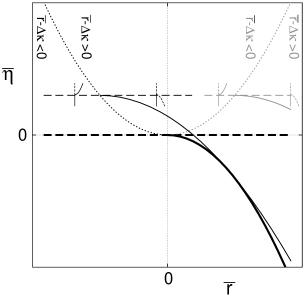
Figure 2: Sketch of a partial bifurcation diagram of the amplitude equation (2) in the $\bar{r}$–$\bar{\eta}$ plane. The thick broken line indicates the instability of the trivial state. The thin broken line represents the bifurcation of plane waves from the trivial state for a wave number $\kappa$ with $\Delta\kappa>0$ (cf. eq.(45)). The pitchfork like inserts indicate whether the bifurcations are sub– or supercritical and the thin dotted line gives the transition for all wavenumbers (cf. eq.(47)). The thin solid line marks the saddle node bifurcation for the plane wave (cf. eq.(49)). The corresponding features for the wavenumber $-\kappa$ are displayed in grey. Finally the thick solid line marks the envelope of saddle node bifurcation lines for all wavenumbers (cf. eq.(51)).

The region of existence of a plane wave solution, which is bounded by eq.(49) extends beyond the stability region of the trivial state.

We now have to perform the analysis presented above for every wavenumber $\kappa$. The region where plane wave solutions exist is given by the union of the regions described above. Hence its boundary is determined by the envelope of the curves (49) for all wavenumbers. It is easily computed as (cf. fig.2)

$$\bar{\eta}=-D\bar{r}^{2}/[4D(-s)-\Delta^{2}],\quad(\bar{r}>0),\hskip 25.0pt\mbox{if }|\Delta|<\Delta_{c}:=2\sqrt{D(-s)}\quad.$$ (51)

If $|\Delta|$ approaches $\Delta_{c}$ the parabola (51) degenerates with the negative $\bar{\eta}$–axis. For $|\Delta|>\Delta_{c}$ no boundary exists at all, so that for every $\bar{\eta}<0$ there exist plane wave solutions.

In summary, the scenario for $|\Delta|<\Delta_{c}$ resembles the sub–supercritical transition in low dimensional dynamical systems, where a saddle–node bifurcation line is typically born. But in the extended case this behaviour is destroyed at $|\Delta|=\Delta_{c}$, which can be viewed as a codimension three bifurcation point.

Yet we have not claimed the stability of the plane wave solutions. A linear stability analysis according to $\bar{A}=\alpha_{k}\exp({\mathrm{i}}\kappa\xi)(1+\delta\beta)$ yields the linear equation

$$\partial_{\tau}\delta\beta = \bar{\eta}\delta\beta+D(-\kappa^{2}\delta\beta+{\mathrm{i}}2\kappa\partial_{\xi}\delta\beta+\partial_{\xi}^{2}\delta\beta)+\bar{r}|\alpha_{\kappa}|^{2}(\delta\beta^{*}+2\delta\beta)+s|\alpha_{\kappa}|^{4}(2\delta\beta^{*}+3\delta\beta)$$ (52)

$$- (g-d)\kappa|\alpha_{\kappa}|^{2}(2\delta\beta+\delta\beta^{*})+{\mathrm{i}}g|\alpha_{\kappa}|^{2}\partial_{\xi}\delta\beta+{\mathrm{i}}d|\alpha_{\kappa}|^{2}\partial_{\xi}\delta\beta^{*}\quad.$$

Splitting into real and imaginary parts and and taking the fixed point equation (44) into account the corresponding real two dimensional system reads

$$\partial_{\tau}\left(\begin{array}[]{c}\mbox{Re}\delta\beta\\ \mbox{Im}\delta\beta\end{array}\right)=\left(\begin{array}[]{cc}2(\bar{r}-\Delta\kappa)|\alpha_{\kappa}|^{2}+4s|\alpha_{\kappa}|^{4}+D\partial_{\xi}^{2}&(-2D\kappa-\Delta|\alpha_{\kappa}|^{2})\partial_{\xi}\\ (2D\kappa+(g+d)|\alpha_{\kappa}|^{2})\partial_{\xi}&D\partial_{\xi}^{2}\end{array}\right)\left(\begin{array}[]{c}\mbox{Re}\delta\beta\\ \mbox{Im}\delta\beta\end{array}\right)\quad.$$ (53)

Analysing the stability in terms of plane waves $\exp({\mathrm{i}}\omega\xi)$ yields a two–dimensional eigenvalue problem, where the trace and the determinant of the corresponding matrix read

$$\mathop{\mathrm{T}r}\nolimits_{\omega} = 2\left[-D\omega^{2}+(\bar{r}-\Delta\kappa)|\alpha_{\kappa}|^{2}+2s|\alpha_{\kappa}|^{4}\right]$$ (54)

$$\mbox{Det}_{\omega} = \omega^{2}\left[D^{2}\omega^{2}-2D\left(\bar{r}-\Delta\kappa\right)|\alpha_{\kappa}|^{2}-4Ds|\alpha_{\kappa}|^{4}\right.$$ (55)

$$- \left.\left(2D\kappa+(g+d)|\alpha_{\kappa}|^{2}\right)\left(2D\kappa+\Delta|\alpha_{\kappa}|^{2}\right)\right]\quad.$$

Stability requires $\mathop{\mathrm{T}r}\nolimits_{\omega}<0$ and $\mbox{Det}_{\omega}\geq 0$ for all wavenumbers $\omega$. Owing to the simple dependence on $\omega$ the condition on the trace results in

$$|\alpha_{\kappa}|^{2}>(\bar{r}-\Delta\kappa)/(-2s)\quad,$$ (56)

which is of course valid if the right hand side is negative. Whenever the right hand side is positive and the parameters are such that plane wave solutions are possible, i. e. we are beyond the saddle node bifurcation line (cf. eqs.(49), (50)), then eq.(48) tells us, that the solution with the larger amplitude obeys the constraint (56), whereas the solution with the smaller amplitude is unstable. Hence we are left with checking the condition on the determinant which results in

$$4D(-s)|\alpha_{\kappa}|^{2}\left[|\alpha_{\kappa}|^{2}-(\bar{r}-\Delta\kappa)/(-2s)\right]-\left(2D\kappa+(g+d)|\alpha_{\kappa}|^{2}\right)\left(2D\kappa+\Delta|\alpha_{\kappa}|^{2}\right)\geq 0\quad.$$ (57)

Due to this condition it is evident, that the stability properties depend on the parameters $g$ and $d$ separately. A complete discussion of the stability using eq.(57) is straightforward but tedious. We do not intend to discuss the full implications of this inequality, but just concentrate on a neighbourhood of the envelope (51) in order to study whether stable solutions are generated at this bifurcation line. For that purpose we fix the wavenumber to $\kappa=-\Delta\bar{r}/(\Delta_{c}^{2}-\Delta^{2})$ which is just the value for which the saddle node bifurcation line touches the envelope (cf. fig.2 and eqs.(48), (49), and (51)) and expand the left hand side of eq.(57) for $\bar{\eta}$ values slightly beyond the envelope (cf. eq.49). We obtain to the leading order the result

$$\left[4D(-s)-2g\Delta\right]|\alpha_{\kappa}|^{2}\left[|\alpha_{\kappa}|^{2}-(\bar{r}-\Delta\kappa)/(-2s)\right]\geq 0\quad.$$ (58)

For the solution with the larger amplitude (cf. eq.(56)) the condition is satisfied provided that $g\Delta<2D(-s)$ holds. Then a stable plane wave occurs at the envelope.

4 Conclusion

We have presented the complete and systematic derivation of the amplitude equation, which governs the transition from sub– to supercritical soft–mode instabilities. Within our approach the general expression for the coefficients and especially their dependence on the system parameters has been obtained. Although these formulas look a little bit lengthy, one should keep in mind that they can be applied to almost every physical situation, and that their evaluation is straightforward in concrete cases.

From the principal point of view it is worth to mention, that the amplitude equation (2) can be derived consistently at all. Such a feature is far from being obvious. To emphasise this point consider the corresponding hard–mode case, i. e. an instability at $q_{c}=0$ with a nonvanishing frequency. A superficial inspection would suggest that the whole derivation goes along the same lines with minor modifications. But if we follow the approach of section 2, we are left at the third order with eq.(25). Since now all expressions are complex valued but the higher order codimension condition requires a vanishing real part only, the secular condition becomes a nonlinear equation. Of course it can be easily integrated to yield the time dependence on the scale $\tau_{1}$ as $A=\tilde{A}\exp[{\mathrm{i}}\mbox{Im}(\rho_{3})|\tilde{A}|^{2}\tau_{1}]$. Here the constant of integration $\tilde{A}$ depends on the slower scales. If one uses this representation in the subsequent orders, then the derivatives with respect to spatial coordinates yield linearly in $\tau_{1}$ increasing terms, since the exponent is space dependent. This feature invalidates the systematic derivation although a semi–quantitative approach has been proposed (cf. the discussion in [10]).

The origin of such difficulties lies in high frequency components which contribute to the secular conditions in low orders and cause an uncontrolled mixing of different time scales. Similar phenomena are well known in the problem of counterpropagating waves, where a formal derivation is still possible and a nonlocal coupling in the amplitude equation is generated [11]. For the degenerated hard–mode instability we expect finally similar effects but further investigations are needed. Nevertheless these considerations emphasise again the necessity of careful derivations of amplitude equations to supplement phenomenological approaches.

Concerning the behaviour beyond the sub–supercritical soft–mode instability we stress that without an odd derivative term a potential system occurs. Hence that kind of term is responsible for a persistent time evolution beyond the threshold. In addition, we mention that the difference $\Delta$ between the normal and the odd derivative term determines the domain of existence of spatially periodic patterns in the vicinity of the threshold. These properties again show that the behaviour beyond the instability depends crucially on the actual numerical values of the coefficients.

Appendix A Inhomogeneous part

For convenience we list in this appendix the inhomogeneous parts, which occur in each stage of the derivation of the amplitude equation. For notational simplicity the same label is assigned to the components at each order and we use an overbar to denote negative indices $\bar{n}=-n$. All the abbreviations which we introduce are real valued.

If we insert eq.(16) into the equation of motion (3) and observe the expansion (18) we obtain at the order $\mathop{\mathrm{O}}\nolimits(\varepsilon^{1/2})$

$$0=\underline{\underline{L}}(q_{c})\underline{u}_{c}\exp(iq_{c}x)A+c.c.$$ (A1)

since the spatial derivatives act on the plane wave only. This condition is fulfilled by virtue of the eigenvalue equation for the critical mode (6).

At the order $\mathop{\mathrm{O}}\nolimits(\varepsilon)$ one obtains a contribution from the temporal and spatial derivatives acting on $\underline{\Phi}_{2}$ and one contribution from the quadratic nonlinearity (8) at $\underline{\mu}=\underline{\mu}_{c}$ with the derivatives acting only on the plane waves. Taking the abbreviation (11) into account the result reads

$$\partial_{t}\underline{\Phi}_{2} = {\cal L}\underline{\Phi}_{2}+\sum_{\alpha\beta}C^{(\alpha\beta)}\{\partial_{x}^{\alpha}\underline{\Phi}_{1},\partial_{x}^{\beta}\underline{\Phi}_{1}\}$$ (A2)

$$= {\cal L}\underline{\Phi}_{2}+\underline{C}_{1\bar{1}}(\underline{u}_{c},\underline{u}_{c})|A|^{2}+\left[\underline{C}_{11}(\underline{u}_{c},\underline{u}_{c})\exp(2iq_{c}x)A^{2}+c.c.\right]\quad.$$

Hence in the notation of eq.(20) the nonvanishing Fourier components read

$$\underline{w}_{0}=-2\underline{\underline{L}}(0)\underline{\Gamma}_{20}|A|^{2},\quad\underline{w}_{2}=-\underline{\underline{L}}(2q_{c})\underline{\Gamma}_{22}A^{2}\quad,$$ (A3)

where the abbreviations

$$\underline{\Gamma}_{20}:=-\underline{\underline{L}}(0)^{-1}\underline{C}_{1\bar{1}}(\underline{u}_{c},\underline{u}_{c}),\quad\underline{\Gamma}_{22}:=-\underline{\underline{L}}(2q_{c})^{-1}\underline{C}_{11}(\underline{u}_{c},\underline{u}_{c})$$ (A4)

have been used, and the obvious relation $\underline{w}_{\bar{n}}=\underline{w}_{n}^{*}$ should be noted. The solution of the linear equation (A2), discarding exponentially decaying transients, is given by eq.(24).

At the order $\mathop{\mathrm{O}}\nolimits(\varepsilon^{3/2})$ the time derivative and the linear operator act plainly on $\underline{\Phi}_{3}$. In addition, these derivatives give a contribution when acting on the slow scales of $\underline{\Phi}_{1}$. For the nonlinearities now the quadratic and the cubic terms at $\underline{\mu}=\underline{\mu}_{c}$ contribute

$$\partial_{t}\underline{\Phi}_{3} = {\cal L}\underline{\Phi}_{3}+{\cal L}^{(1)}\underline{\Phi}_{1}+({\cal L}\underline{\Phi}_{1})^{[1]}-\partial_{\tau_{1}}\underline{\Phi}_{1}$$ (A5)

$$+ \sum_{\alpha\beta}2C^{(\alpha\beta)}\{\partial_{x}^{\alpha}\underline{\Phi}_{2},\partial_{x}^{\beta}\underline{\Phi}_{1}\}+\sum_{\alpha\beta\gamma}D^{(\alpha\beta\gamma)}\{\partial_{x}^{\alpha}\underline{\Phi}_{1},\partial_{x}^{\beta}\underline{\Phi}_{1},\partial_{x}^{\gamma}\underline{\Phi}_{1}\}\quad.$$

Here the notation $({\cal L}\underline{\Phi}_{1})^{[1]}$ means that the derivatives have to be evaluated at the first order in $\varepsilon$. All other derivatives with respect to $x$ are understood at fixed values of $\xi_{k}$. Taking the relation $(\partial_{x}^{\alpha}\exp(iq_{c}x)A)^{[1]}=\alpha(iq_{c})^{\alpha-1}\exp(iq_{c}x)\partial_{\xi_{1}}A$ into account the third contribution on the right hand side is expressed in terms of the derivative of the matrix (5) with respect to $k$. If we evaluate the nonlinear contribution with the help of the solution (24) of the preceding order and recast all contributions into the form (20) we get

$$\underline{w}_{0} = -2\underline{\underline{L}}(0)\underline{\Gamma}_{20}AB^{*}$$

$$\underline{w}_{1} = -\underline{u}_{c}\partial_{\tau_{1}}A+\underline{\underline{L}}^{(1)}(q_{c})\underline{u}_{c}A-{\mathrm{i}}\underline{\underline{L}}^{\prime}(q_{c})\underline{u}_{c}\partial_{\xi_{1}}A$$

$$+ \left[2\underline{C}_{2\bar{1}}(\underline{\Gamma}_{22},\underline{u}_{c})+4\underline{C}_{10}(\underline{u}_{c},\underline{\Gamma}_{20})+3\underline{D}_{11\bar{1}}(\underline{u}_{c},\underline{u}_{c},\underline{u}_{c})\right]|A|^{2}A$$

$$\underline{w}_{2} = -2\underline{\underline{L}}(2q_{c})\underline{\Gamma}_{22}AB$$

$$\underline{w}_{3} = -\underline{\underline{L}}(3q_{c})\underline{\Gamma}_{33}A^{3}$$ (A6)

with the abbreviation

$$\underline{\Gamma}_{33}:=-\underline{\underline{L}}^{-1}(3q_{c})\left[2\underline{C}_{21}(\underline{\Gamma}_{22},\underline{u}_{c})+\underline{D}_{111}(\underline{u}_{c},\underline{u}_{c},\underline{u}_{c})\right]$$ (A7)

Here $\underline{\underline{L}}^{\prime}(k)$ denotes the derivative with respect to $k$. The nonsecular solution discarding transients is given by eq.(29) where the abbreviations

$$\underline{\Gamma}_{31}:=-\underline{\underline{L}}_{c}^{-1}\left[2\underline{C}_{2\bar{1}}(\underline{\Gamma}_{22},\underline{u}_{c})+4\underline{C}_{10}(\underline{u}_{c},\underline{\Gamma}_{20})+3\underline{D}_{11\bar{1}}(\underline{u}_{c},\underline{u}_{c},\underline{u}_{c})\right]$$ (A8)

$$\underline{\gamma}_{31}^{a}:=-\underline{\underline{L}}_{c}^{-1}\underline{\underline{L}}^{\prime}(q_{c})\underline{u}_{c}=(\underline{\underline{1}}-|\underline{u}_{c}\rangle\langle\underline{v}_{c}|)\partial_{k}\underline{u}_{k}(\underline{\mu}_{c})|_{k=q_{c}}$$ (A9)

$$\underline{\gamma}_{31}^{b}:=-\underline{\underline{L}}_{c}^{-1}\underline{\underline{L}}^{(1)}(q_{c})\underline{u}_{c}=(\underline{\underline{1}}-|\underline{u}_{c}\rangle\langle\underline{v}_{c}|)(\underline{\mu}^{(1)}\partial_{\underline{\mu}})\underline{u}_{q_{c}}(\underline{\mu})|_{\underline{\mu}=\underline{\mu}_{c}}\quad.$$ (A10)

have been introduced.

Proceeding to the order $\mathop{\mathrm{O}}\nolimits(\varepsilon^{2})$ one has to observe that in addition the parameter dependence of the quadratic term has to be taken into account (cf. eq.(15)). Denoting the corresponding directional derivative by $C^{(\alpha\beta)(1)}=(\underline{\mu}^{(1)}\partial_{\underline{\mu}})C^{(\alpha\beta)}_{\underline{\mu}}|_{\underline{\mu}=\underline{\mu}_{c}}$ the equation reads

$$\partial_{t}\underline{\Phi}_{4} = {\cal L}\underline{\Phi}_{4}+{\cal L}^{(1)}\underline{\Phi}_{2}+({\cal L}\underline{\Phi}_{2})^{[1]}-\partial_{\tau_{1}}\underline{\Phi}_{2}$$ (A11)

$$+ \sum_{\alpha\beta}\left[C^{(\alpha\beta)}\{\partial_{x}^{\alpha}\underline{\Phi}_{2},\partial_{x}^{\beta}\underline{\Phi}_{2}\}+2C^{(\alpha\beta)}\{\partial_{x}^{\alpha}\underline{\Phi}_{3},\partial_{x}^{\beta}\underline{\Phi}_{1}\}\right.$$

$$\left.+\,2C^{(\alpha\beta)}\{(\partial_{x}^{\alpha}\underline{\Phi}_{1})^{[1]},\partial_{x}^{\beta}\underline{\Phi}_{1}\}+C^{(\alpha\beta)(1)}\{\partial_{x}^{\alpha}\underline{\Phi}_{1},\partial_{x}^{\beta}\underline{\Phi}_{1}\}\right]$$

$$+ \sum_{\alpha\beta\gamma}3D^{(\alpha\beta\gamma)}\{\partial_{x}^{\alpha}\underline{\Phi}_{2},\partial_{x}^{\beta}\underline{\Phi}_{1},\partial_{x}^{\gamma}\underline{\Phi}_{1}\}+\sum_{\alpha\beta\gamma\delta}E^{(\alpha\beta\gamma\delta)}\{\partial_{x}^{\alpha}\underline{\Phi}_{1},\partial_{x}^{\beta}\underline{\Phi}_{1},\partial_{x}^{\gamma}\underline{\Phi}_{1},\partial_{x}^{\delta}\underline{\Phi}_{1}\}\quad.$$

Inserting the solutions of the preceding orders and performing the derivatives we obtain for the Fourier modes up to wavenumber $2q_{c}$

$$\underline{w}_{0} = \underline{\underline{L}}(0)\left[-2\underline{\Gamma}_{20}\left(AC^{*}+A^{*}C+|B|^{2}\right)-2{\mathrm{i}}\underline{\gamma}_{40}^{a}\left(A\partial_{\xi_{1}}A^{*}-A^{*}\partial_{\xi_{1}}A\right)\right.$$

$$- \left.\underline{\Gamma}_{40}|A|^{4}-2\underline{\gamma}_{40}^{b}|A|^{2}\right]$$

$$\underline{w}_{1} = -\underline{u}_{c}\partial_{\tau_{1}}B+\underline{\underline{L}}^{(1)}(q_{c})\underline{u}_{c}B-{\mathrm{i}}\underline{\underline{L}}^{\prime}(q_{c})\underline{u}_{c}\partial_{\xi_{1}}B$$

$$+ \left[2\underline{C}_{2\bar{1}}(\underline{\Gamma}_{22},\underline{u}_{c})+4\underline{C}_{10}(\underline{u}_{c},\underline{\Gamma}_{20})+3\underline{D}_{11\bar{1}}(\underline{u}_{c},\underline{u}_{c},\underline{u}_{c})\right]\left[2|A|^{2}B+A^{2}B^{*}\right]$$

$$\underline{w}_{2} = -\underline{\underline{L}}(2q_{c})\left[\underline{\gamma}_{42}^{b}A^{2}+2\underline{\Gamma}_{22}AC+2{\mathrm{i}}\underline{\gamma}^{a}_{42}A\partial_{\xi_{1}}A+\underline{\Gamma}_{42}A^{*}A^{3}+\underline{\Gamma}_{22}B^{2}\right]$$ (A12)

with the abbreviations

$$\underline{\Gamma}_{40} := -\underline{\underline{L}}(0)^{-1}\left[2\underline{C}_{1\bar{1}}(\underline{\Gamma}_{31},\underline{u}_{c})+2\underline{C}_{1\bar{1}}(\underline{u}_{c},\underline{\Gamma}_{31})+2\underline{C}_{2\bar{2}}(\underline{\Gamma}_{22},\underline{\Gamma}_{22})+4\underline{C}_{00}(\underline{\Gamma}_{20},\underline{\Gamma}_{20})\right.$$ (A13)

$$+ 3\underline{D}_{11\bar{2}}(\underline{u}_{c},\underline{u}_{c},\underline{\Gamma}_{22})+3\underline{D}_{2\bar{1}\bar{1}}(\underline{\Gamma}_{22},\underline{u}_{c},\underline{u}_{c})+12\underline{D}_{10\bar{1}}(\underline{u}_{c},\underline{\Gamma}_{20},\underline{u}_{c})$$

$$+ \left.6\underline{E}_{11\bar{1}\bar{1}}(\underline{u}_{c},\underline{u}_{c},\underline{u}_{c},\underline{u}_{c})\right]$$

$$\underline{\gamma}^{a}_{40} := -\underline{\underline{L}}(0)^{-1}\ \left[-\underline{\underline{L}}^{\prime}(0)\underline{\Gamma}_{20}+\underline{C}_{1\bar{1}}(\underline{u}_{c},\underline{\gamma}^{a}_{31})-\tilde{\underline{C}}_{\bar{1}1}(\underline{u}_{c},\underline{u}_{c})\right]$$ (A14)

$$\underline{\gamma}^{b}_{40} := -\underline{\underline{L}}(0)^{-1}\left[\underline{C}_{1\bar{1}}(\underline{\gamma}^{b}_{31},\underline{u}_{c})+\underline{C}_{1\bar{1}}(\underline{u}_{c},\underline{\gamma}^{b}_{31})+\underline{\underline{L}}^{(1)}(0)\ \underline{\Gamma}_{20}+\underline{C}_{1\bar{1}}^{(1)}(\underline{u}_{c},\underline{u}_{c})\right]$$ (A15)

$$\underline{\Gamma}_{42} := -\underline{\underline{L}}(2q_{c})^{-1}\left[2\underline{C}_{11}(\underline{\Gamma}_{31},\underline{u}_{c})+2\underline{C}_{3\bar{1}}(\underline{\Gamma}_{33},\underline{u}_{c})+4\underline{C}_{20}(\underline{\Gamma}_{22},\underline{\Gamma}_{20})\right.$$ (A16)

$$+ \left.6\underline{D}_{110}(\underline{u}_{c},\underline{u}_{c},\underline{\Gamma}_{20})+6\underline{D}_{21\bar{1}}(\underline{\Gamma}_{22},\underline{u}_{c},\underline{u}_{c})+6\underline{E}_{111\bar{1}}(\underline{u}_{c},\underline{u}_{c},\underline{u}_{c},\underline{u}_{c})\right]$$

$$\underline{\gamma}^{a}_{42} := -\underline{\underline{L}}(2q_{c})^{-1}\left[-\underline{\underline{L}}^{\prime}(2q_{c})\underline{\Gamma}_{22}-\underline{C}_{11}(\underline{\gamma}^{a}_{31},\underline{u}_{c})-\tilde{\underline{C}}_{11}(\underline{u}_{c},\underline{u}_{c})\right]$$ (A17)

$$\underline{\gamma}^{b}_{42} := -\underline{\underline{L}}(2q_{c})^{-1}\left[2\underline{C}_{11}(\underline{u}_{c},\underline{\gamma}^{b}_{31})+\underline{\underline{L}}^{(1)}(2q_{c})\underline{\Gamma}_{22}+\underline{C}_{11}^{(1)}(\underline{u}_{c},\underline{u}_{c})\right]$$ (A18)

and

$$\tilde{\underline{C}}_{mn}(\underline{u},\underline{v}):={\mathrm{i}}\sum_{\alpha\beta}\alpha({\mathrm{i}}mq_{c})^{\alpha-1}({\mathrm{i}}nq_{c})^{\beta}\underline{C}^{(\alpha\beta)}\{\underline{u},\underline{v}\}\quad.$$ (A19)

The nonsecular solution of eq.(A11) up to Fourier modes $\pm 2q_{c}$ is then given by eq.(32). We remark that, if the definitions (A4) are understood in terms of the full parameter dependent quantities and eigenvectors (cf. eqs.(5), (11), and (6)), then the abbreviations (A15) and (A18) obey, taking relation (A10) into account

$$\underline{\gamma}_{40}^{b} = \left.(\underline{\mu}^{(1)}\partial_{\underline{\mu}})\underline{\Gamma}_{20}\right|_{\underline{\mu}=\underline{\mu}_{c}}-\underline{\Gamma}_{20}\left(\langle\underline{v}_{c}|(\underline{\mu}^{(1)}\partial_{\underline{\mu}})\underline{u}_{q_{c}}(\underline{\mu})|_{\underline{\mu}=\underline{\mu}_{c}}\rangle+c.c.\right)$$ (A20)

$$\underline{\gamma}_{42}^{b} = \left.(\underline{\mu}^{(1)}\partial_{\underline{\mu}})\underline{\Gamma}_{22}\right|_{\underline{\mu}=\underline{\mu}_{c}}-2\underline{\Gamma}_{22}\langle\underline{v}_{c}|(\underline{\mu}^{(1)}\partial_{\underline{\mu}})\underline{u}_{q_{c}}(\underline{\mu})|_{\underline{\mu}=\underline{\mu}_{c}}\rangle\quad.$$ (A21)

Finally at the order $\mathop{\mathrm{O}}\nolimits(\varepsilon^{5/2})$ we end up with

$$\partial_{t}\underline{\Phi}_{5} = {\cal L}\underline{\Phi}_{5}+{\cal L}^{(1)}\underline{\Phi}_{3}+{\cal L}^{(2)}\underline{\Phi}_{1}+({\cal L}\underline{\Phi}_{3})^{[1]}-\partial_{\tau_{1}}\underline{\Phi}_{3}+({\cal L}\underline{\Phi}_{1})^{[2]}-\partial_{\tau_{2}}\underline{\Phi}_{1}+({\cal L}^{(1)}\underline{\Phi}_{1})^{[1]}$$ (A22)

$$+ \sum_{\alpha\beta}\left[2C^{(\alpha\beta)}\{\partial_{x}^{\alpha}\underline{\Phi}_{4},\partial_{x}^{\beta}\underline{\Phi}_{1}\}+2C^{(\alpha\beta)}\{\partial_{x}^{\alpha}\underline{\Phi}_{3},\partial_{x}^{\beta}\underline{\Phi}_{2}\}\right.$$

$$\left.+\,2C^{(\alpha\beta)}\{(\partial_{x}^{\alpha}\underline{\Phi}_{2})^{[1]},\partial_{x}^{\beta}\underline{\Phi}_{1}\}+2C^{(\alpha\beta)}\{(\partial_{x}^{\alpha}\underline{\Phi}_{1})^{[1]},\partial_{x}^{\beta}\underline{\Phi}_{2}\}+2C^{(\alpha\beta)(1)}\{\partial_{x}^{\alpha}\underline{\Phi}_{2},\partial_{x}^{\beta}\underline{\Phi}_{1}\}\right]$$

$$+ \sum_{\alpha\beta\gamma}\left[3D^{(\alpha\beta\gamma)}\{\partial_{x}^{\alpha}\underline{\Phi}_{3},\partial_{x}^{\beta}\underline{\Phi}_{1},\partial_{x}^{\gamma}\underline{\Phi}_{1}\}+3D^{(\alpha\beta\gamma)}\{\partial_{x}^{\alpha}\underline{\Phi}_{2},\partial_{x}^{\beta}\underline{\Phi}_{2},\partial_{x}^{\gamma}\underline{\Phi}_{1}\}\right.$$

$$\left.+\,3D^{(\alpha\beta\gamma)}\{(\partial_{x}^{\alpha}\underline{\Phi}_{1})^{[1]},\partial_{x}^{\beta}\underline{\Phi}_{1},\partial_{x}^{\gamma}\underline{\Phi}_{1}\}+D^{(\alpha\beta\gamma)(1)}\{\partial_{x}^{\alpha}\underline{\Phi}_{1},\partial_{x}^{\beta}\underline{\Phi}_{1},\partial_{x}^{\gamma}\underline{\Phi}_{1}\}\right]$$

$$+ \sum_{\alpha\beta\gamma\delta}4E^{(\alpha\beta\gamma\delta)}\{\partial_{x}^{\alpha}\underline{\Phi}_{2},\partial_{x}^{\beta}\underline{\Phi}_{1},\partial_{x}^{\gamma}\underline{\Phi}_{1},\partial_{x}^{\delta}\underline{\Phi}_{1}\}$$

$$+ \sum_{\alpha\beta\gamma\delta\epsilon}F^{(\alpha\beta\gamma\delta\epsilon)}\{\partial_{x}^{\alpha}\underline{\Phi}_{1},\partial_{x}^{\beta}\underline{\Phi}_{1},\partial_{x}^{\gamma}\underline{\Phi}_{1},\partial_{x}^{\delta}\underline{\Phi}_{1},\partial_{x}^{\epsilon}\underline{\Phi}_{1}\}\quad.$$

As before $D^{(\alpha\beta\gamma)(1)}$ denotes the directional derivative and $({\cal L}\underline{\Phi}_{1})^{[2]}$ indicates that spatial derivatives have to be evaluated at order $\mathop{\mathrm{O}}\nolimits(\varepsilon^{2})$. Inserting the previous orders and performing the derivatives the Fourier mode $\underline{w}_{1}$ of the inhomogeneous part of eq.(A22) is evaluated and yields after some algebra the secular condition (2.2), taking the abbreviation

$$\tilde{\underline{D}}_{lmn}(\underline{u},\underline{v},\underline{w}):={\mathrm{i}}\sum_{\alpha\beta\gamma}\alpha({\mathrm{i}}lq_{c})^{\alpha-1}({\mathrm{i}}mq_{c})^{\beta}({\mathrm{i}}nq_{c})^{\gamma}\underline{D}^{(\alpha\beta\gamma)}\{\underline{u},\underline{v},\underline{w}\}$$ (A23)

into account.

References

References

• [1] Cross M C and Hohenberg P C 1993 Rev. Mod. Phys. 65 851
• [2] Guckenheimer J and Holmes P 1986 Nonlinear Oscillations, Dynamical Systems, and Bifurcations of Vector Fields (New York: Springer)
• [3] Manneville P 1990 Dissipative Structure and Weak Turbulence (San Diego: Acad. Press)
• [4] Collet P 1994 Nonlinearity 7 1175
• [5] Becerril R and Swift J B 1997 Phys. Rev. E 55 6270
• [6] Deissler R J and Brand H R Phys. Lett. A 1990 146 252
• [7] van Saarloos W and Hohenberg P C 1992 Physica D 56 303; Erratum 1993 Physica D 69 209
• [8] Eckhaus W and Iooss G 1989 Physica D 39 124
• [9] Doelman A and Eckhaus W 1991 Physica D 53 249
• [10] Brand H, Lomdahl P S, and Newell A C Phys. Lett. A 1986 118 67
• [11] Knobloch E and de Luca J 1990 Nonlinearity 3 975