[
Hexagons and Interfaces in a Vibrated Granular Layer
Abstract
The order parameter model based on parametric Ginzburg-Landau equation is used to describe high acceleration patterns in vibrated layer of granular material. At large amplitude of driving both hexagons and interfaces emerge. Transverse instability leading to formation of “decorated” interfaces and labyrinthine patterns, is found. Additional sub-harmonic forcing leads to controlled interface motion.
pacs:
PACS: 47.54.+r, 47.35.+i,46.10.+z,83.70.Fn] Driven granular materials often manifest collective fluid-like behavior: convection, surface waves, and pattern formation (see e.g. [1]). One of the most fascinating examples of this collective dynamics is the appearance of long-range coherent patterns and localized excitations in vertically-vibrated thin granular layers [2, 3, 4]. The particular pattern is determined by the interplay between driving frequency and acceleration of the container ( is the amplitude of oscillations, is the gravity acceleration) [2, 3]. Patterns appear at almost independently of the driving frequency . At small frequencies [5] the transition is subcritical (hysteretic), leading to formation of either squares or localized excitations such as individual oscillons and various bound states of oscillons. For higher frequencies the transition is supercritical, and stripes appear first. Both squares and stripes oscillate at half of the driving frequency . At higher acceleration (), stripes and squares become unstable, and hexagons appear instead. Further increase of acceleration at converts hexagons into a domain-like structure of flat layers oscillating with frequency with opposite phases. Depending on parameters, interfaces separating flat domains, are either smooth or ”decorated” by periodic undulations. Undulations slowly grow with time and eventually become quasi-periodic labyrinthine patterns. For various quarter-harmonic patters emerge.
The problem of pattern formation in thin layers of granular material was studied by several groups. While molecular dynamics simulations [6] and hydrodynamic and phenomenological models [7] reproduced certain experimental features, neither of them offered a systematic description of the whole rich variety of the observed phenomena. In Ref. [8] we introduced the order parameter characterizing the complex amplitude of sub-harmonic oscillations. The equations of motion following from the symmetry arguments and mass conservation reproduced essential phenomenology of patterns near the threshold of primary bifurcation: stripes, squares and oscillons.
In this Letter we describe high acceleration patterns on the basis the order parameter model. We show that at large amplitude of driving both hexagons and interfaces emerge. We find morphological instability leading to formation of “decorated” interfaces and labyrinthine patterns. We develop the description of the labyrinths in terms of nonlocal contour dynamics. Additional sub-harmonic forcing leads to the motion of the interface with the direction controlled by relative phases of harmonic and sub-harmonic components of forcing.
The essential of the model [8, 9] is the order parameter equation for the complex amplitude of parametric layer oscillations at the frequency . In general, is coupled with the the average thickness of the layer . However, at high frequencies () the coupling between and becomes unimportant, and the model can be reduced to a single order-parameter equation
| (1) |
Eq.(1) describes the evolution of the order parameter for the parametric instability in spatially-extended systems (see [10, 11]). Linear terms in this equation are obtained from the complex growth rate for infinitesimal periodic layer perturbations . Expanding for small , and keeping only two leading terms in the expansion we reproduce the linear terms in Eq. (1), where and , where . The term characterizes the effect of driving at the resonance frequency. The term accounts for nonlinear saturation of waves at finite amplitude.
It is convenient to shift the phase of the complex order parameter via with . The equations for real and imaginary part are:
| (2) | |||||
| (3) |
where . At , Eqs. (2),(3) has only one trivial uniform state , At , two new uniform states appear, . The onset of these states corresponds to the period doubling of the layer flights sequence, observed in experiments [2] and predicted by the simple inelastic ball model [2, 12]. Signs reflect two relative phases of layer flights with respect to container vibrations.
First we analyze the stability of the state with respect to perturbations with wavenumber , The uniform state loses its stability with respect to periodic modulations with the wavenumber at (correspondingly, ), where
| (4) | |||||
| (5) |
Small perturbations with all directions of the wavevector grow with the same rate. The resultant selected pattern is determined by the nonlinear competition between the modes. In the presence of the reflection symmetry , quadratic nonlinearity is absent, and cubic nonlinearity favors stripes corresponding to a single mode. Near the fixed points the reflection symmetry for perturbations is broken, and hexagons emerge at the threshold of instability. To clarify this point we perform weakly-nonlinear analysis of Eqs. (2),(3) for , and . At , the variables and are related as in linear system:
| (6) | |||||
| (7) |
Corresponding adjoint eigenvector is
| (8) |
Substituting Eq. (7) into Eqs. (2),(3) and performing the orthogonalization, we obtain equations for the slowly-varying complex amplitudes , (we assume only three waves with triangular symmetry, favored by quadratic nonlinearity)
| (9) | |||||
| (10) |
where the coefficients are
| (11) |
Eqs. (10) are well-studied (see [13]). There are three critical values of : and . The hexagons are stable for , and the stripes are stable for . Thus, near the model exhibit stable hexagons [14]. Since we have two symmetric fixed points, both up- and down-hexagons co-exist. For smaller stripes are stable, and for larger , flat layers are stable, in agreement with observations[3, 16]. The above analysis requires the values of to be small. For parameters , this requirement is satisfied for , but not for . The estimates can be improved by substituting at instead of in (11). The resulting range of stable hexagons is plotted in the phase diagram (see Fig. 1).
At , Eqs. (2),(3) have an interface solution connecting two uniform states . For this solution is of the form . For the solution is available only numerically. In order to investigate the stability of the interface, we consider the perturbed solution . For we obtain linear equations
| (12) |
| (15) |
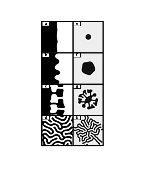
In order to determine the spectrum of eigenvalues one has to solve Eq. (12) along with stationary Eqs. (2),(3). Using numerical matching-shooting technique, we have obtained positive eigenvalues corresponding to interface instability. This instability is confirmed by direct numerical simulations of Eq.(1). An example of the evolution of slightly perturbed interface is shown in Fig. 2. Small perturbations grow to form a “decorated” interface similar to [17], with time these decorations evolve slowly and eventually form a labyrinthine pattern [16].
The neutral curve for this instability can be determined as follows. Numerical analysis shows that at the threshold the most unstable wavenumber is and we can expect that for . Expanding Eqs.(12) in power series of : in the zeroth order in we obtain . The corresponding solution is the translation mode . In the first order in we arrive at the linear inhomogeneous problem
| (16) |
A bounded solution to Eq. (16) exists if the r.h.s. is orthogonal to the localized mode of the adjoint operator . The orthogonality condition fixes the relation between and :
| (17) |
The instability, corresponding to the negative surface tension of the interface, onsets at . The neutral curve is shown in Fig. 1. This instability leads to so called “decorated” interfaces (see Fig. 2,a). At the nonlinear stage the undulations grow and form labyrinthine patterns (Fig. 2, b-d). The evolution of the interface can be investigated near the line (see Fig. 1). In the vicinity of this line and . in the leading order we can obtain from Eq. (3) , and Eq. (2) yields
| (18) |
Rescaling the variables , we can reduce Eq. (1) to the Swift-Hohenberg equation (SHE)
| (19) |
where . This equation is simpler than Eq. (1), however it captures many essential features of the original system dynamics, including existence and stability of stripes and hexagons in different parameter regions (see[15]), existence of the interface solutions, interface instability and emergence of labyrinthine patterns. Indeed, simple analysis shows that the growth rate of the instability of the uniform state as a function of the perturbation wavenumber is determined by the formula , so it becomes unstable at at critical wavenumber . As in the original model, near the threshold of this instability, subcritical hexagonal patterns are preferred. Interface stability can also be analyzed more simply as the linearized operator corresponding to the model (19) is self-adjoint. The threshold value is obtained from the following solvability condition
| (20) |
We derived the equation for the position of the curved interface parameterized by its arclength . The solution is sought for in the form , where is the unit normal vector, is the 1D interface solution and is the correction due to interaction with the remote parts of the interface. This correction can be obtained from the linearized SHE in the far field. Substituting this solution in the SHE (19), we obtained the equation for the interface velocity ,
| (21) |
where is the local interface curvature, is an interface “mass” per unit length, and is the surface tension, and . Coefficient is determined from the matching with the asymptotic of one-dimensional interface solution. Eq.(21) is similar to that of Ref. [18]. The first term in the r.h.s. of (21) at describes the destabilizing effect of negative surface tension, and the Biot-Savart type integral accounts for non-local interactions among parts of the interface. According to Ref.[18], combination of these effects gives rise to labyrinthine patterns. Since here is complex, function oscillates, and interfaces form bound states at the distance ). The characteristic wavelength of labyrintine patterns is and is different from the most unstable wavelength of the original interface instability. This difference is evident from Fig. 2 which shows snapshots of the interface dynamics.
In the region of stability () for the original model Eq. (1) the interface is stationary due to symmetry. However, if the plate oscillates with two frequencies, and , the symmetry between two states connected by the interface, is broken, and interface moves. The velocity of interface motion depends on the relative phase of the sub-harmonic forcing with respect to the forcing at . This effect can be described by the additional term in Eq. (1), where characterizes the amplitude of the sub-harmonic pumping, and determines its relative phase. For small , we look for moving interface solution in the form . and . Solvability condition yields the following expression for the interface velocity
| (22) |
The explicit answer is possible to obtain for when , and , which yields the interface velocity . In general, , , and hence , can be found numerically. The interface velocity as function of is shown in Fig. 3.
We have shown that large acceleration patterns are captured by the generic parametric Ginzburg-Landau equation (1). The structure of the phase diagram Fig.1 is qualitatively similar to that of experiments Refs.[2, 16, 17] for high frequencies of vibration. Increasing vibration amplitude leads to transition from a trivial state to stripes, hexagons, decorated interfaces, and finally, to stable interfaces. In experiments, at yet higher , quarter-harmonic patterns appear, however these patterns are not described by our model. Transition from unstable to stable interfaces also occurs with decreasing (increasing vibration frequency ), in agreement with Ref.[16, 17]. In our model, the interface instability leads to labyrinthine patterns, however it seems that in experiments this instability sometimes saturates to provide stationary “decorations”. Presumably, this saturation is caused by the weak interaction with the density field neglected here. For additional sub-harmonic driving the model predicts steady moving interfaces with the direction of motion controlled by the phase of the sub-harmonic component. Experimental study of the controlled interface motion will be reported elsewhere [19].
We acknowledge useful discussions with H. Swinney, R. Behringer, H. Jaeger and R. Goldstein. This work was supported by the US DOE under grants DE-FG03-95ER14516, DE-FG03-96ER14592, W-31-109-ENG-38, and by NSF, STCS #DMR91-20000.
![[Uncaptioned image]](/html/patt-sol/9802004/assets/x1.png)
REFERENCES
- [1] H. M. Jaeger, S.R. Nagel and R. P. Behringer, Physics Today 49, 32 (1996); Rev. Mod. Phys. 68, 1259 (1996).
- [2] F. Melo, P. Umbanhowar and H.L. Swinney, Phys. Rev. Lett. 72, 172 (1994); ibid 75, 3838 (1995)
- [3] P. B.Umbanhowar, F. Melo and H.L. Swinney, Nature 382, 793 (1996).
- [4] T. H. Metcalf, J. B. Knight, H. M. Jaeger, Physica A 236, 202 (1997).
- [5] In experiments [2, 3] Hz.
- [6] S. Luding et al., Europhys. Lett. 36, 247 (1996); C. Bizon et. al, Phys. Rev. Lett.80, 57 (1998).
- [7] D. Rothman, Phys. Rev. E57 (1998); E. Cerda, F. Melo, and S. Rica, Phys. Rev. Lett.79, 4570 (1997); T. Shinbrot, Nature 389, 574 (1997); J. Eggers and H. Riecke, patt-sol/9801004; S. C. Venkataramani and E. Ott, preprint, 1998.
- [8] L.S. Tsimring and I.S. Aranson, Phys. Rev. Lett. 79, 213 (1997).
- [9] I.S. Aranson, L.T. Tsimring, Physica A 249, 103 (1998).
- [10] W.Zhang and J.Vinals, Phys. Rev. Lett.74, 690 (1995).
- [11] S.V.Kiyashko et al., Phys. Rev. E54, 5037 (1996).
- [12] A. Metha and J.M. Luck, Phys. Rev. Lett.65, 393 (1990).
- [13] M. Cross and P.C. Hohenberg, Rev. Mod. Phys. 65 851 (1993).
- [14] This analysis is similar to that of Ref. [15] where stability of hexagons was demonstrated for the SHE. In a certain limit Eq. (1) can be reduced to SHE (see below).
- [15] G. Dewel et al., Phys. Rev. Lett.74, 4647 (1995).
- [16] P. K. Das and D. Blair, Phys. Lett. A, to appear.
- [17] P.B.Umbanhowar, Ph. Thesis, U.Texas, Austin, 1996.
- [18] D.M. Petrich and R.E. Goldstein, Phys. Rev. Lett.72, 1120 (1996); D.M. Petrich, D.J.Muraki, and R.E. Goldstein, Phys. Rev. E53, 3933 (1996).
- [19] I. Aranson, L. Tsimring, V. Vinokur and U. Welp, in preparation.
![[Uncaptioned image]](/html/patt-sol/9802004/assets/x3.png)