Three basic issues concerning interface dynamics in nonequilibrium pattern formation

Abstract

In these lecture notes, we discuss at an elementary level three themes concerning interface dynamics that play a role in pattern forming systems: (i) We briefly review three examples of systems in which the normal growth velocity is proportional to the gradient of a bulk field which itself obeys a Laplace or diffusion type of equation (solidification, viscous fingers and streamers), and then discuss why the Mullins-Sekerka instability is common to all such gradient systems. (ii) Secondly, we discuss how underlying an effective interface description of systems with smooth fronts or transition zones, is the assumption that the relaxation time of the appropriate order parameter field(s) in the front region is much smaller than the time scale of the evolution of interfacial patterns. Using standard arguments we illustrate that this is generally so for fronts that separate two (meta)stable phases: in such cases, the relaxation is typically exponential, and the relaxation time in the usual models goes to zero in the limit in which the front width vanishes. (iii) We finally summarize recent results that show that so-called “pulled” or “linear marginal stability” fronts which propagate into unstable states have a very slow universal power law relaxation. This slow relaxation makes the usual “moving boundary” or “effective interface” approximation for problems with thin fronts, like streamers, impossible.

Introduction

In this course, and in the two related lectures by Ebert and Brener on their work in [1] and [2], some basic features of the dynamics of growing interfaces in systems which spontaneously form nonequilibrium patterns will be discussed. The analysis of such growth patterns has been an active field of research in the last decade. Moreover, the field is quite diverse, with examples coming from various (sub)disciplines within physics, materials science, and even biology — combustion, convection, crystal growth, chemical waves in excitable media and the formation of Turing patterns, dielectric breakdown, fracture, morphogenesis, etc. We therefore can not hope to review the whole field, but instead will content ourselves with addressing three rather basic topics which we consider to be of rather broad interest, in that they appear (in disguise) in many areas of physics and in some of the related fields. These three themes are explained below.

Our first theme concerns the generality of interfacial growth problems in which the normal growth velocity $v_{n}$ is proportional to the gradient $\nabla\Phi$ of a bulk field $\Phi$ ($v_{n}\sim\nabla\Phi$), and the associated long wavelength instability of such interfaces. As we shall see, one important class of interfacial growth problems with these properties is diffusion limited growth: either the interface grows through the accretion of material via diffusion through one of the adjacent bulk phases, or the growth of the interface is limited by the speed through which, e.g., heat can be transported away from the interface through diffusion. Since the diffusion current near the interface is proportional to the gradient of the appropriate field in the bulk (a concentration field, the temperature, etc.), $v_{n}\sim\nabla\Phi$ in such growth problems. But these are not the only possibilities of how one can have an interface velocity proportional to $\nabla\Phi$. As we will discuss, in viscous fingering an air bubble displaces fluid between two closely spaced plates; as the fluid velocity between the plates is proportional to the gradient of a pressure field $p$, the fact that the air displaces all the fluid means that again at the interface $v_{n}\sim\nabla p$. Likewise, for an ionization front the interface velocity is determined mostly by the drift velocity of electrons in the electric field ${\rm E}=-\nabla\Phi$, where now $\Phi$ is the electrical potential, and so again $v_{n}\sim|\nabla\Phi|$. As we shall see, all such interfacial growth problems where the bulk field itself obeys a Laplace of diffusion equation, exhibit a long wavelength instability, the so-called Mullins-Sekerka instability [3]. This instability lies at the origin of the formation of many nontrivial growth patterns, and Brener and Ebert discussed examples of these at the school. Although this theme is not at all new, it is nevertheless useful to discuss it as an introduction and to stress the generality — the same Mullins-Sekerka instability plays a role in fractal growth processes like Diffusion Limited Aggregation [4]. The above issues are the subject of the first lecture and section 1.

In physics, it is quite common — and often done intuitively without even stating this explicitly — to switch back and forth between a formulation in terms of a mathematically sharp interface (an infinitely thin surface or line at wich the physical fields or their derivatives can show discontinuities) and a formulation in terms of a continuous order parameter field which exhibits a smooth but relatively thin transition zone or domain wall. E.g., we think of the interface between a solid and its melt as a microscopically thin interface, whose width is of the order of a few atomic dimensions. Accordingly, the formulation of the equations that govern the formation of growth patterns of a solid which grows into an undercooled melt on much larger scales $\ell_{\rm pattern}$ have traditionally been formulated in terms of a sharp interface or boundary. The equations, which will be discussed below, are then the diffusion equation for the temperature in the bulk of the liquid and the solid, together with boundary conditions at the interface. These interfacial boundary conditions are a kinematic equation for the growth velocity of the interface in terms of the local interface temperature, and a conservation equation for the heat. The latter expresses that the latent heat released at the interface upon growth of the solid has to be transported away through diffusion into the liquid and the solid. In other words, in an interfacial formulation, the appropriate equations for the bulk fields are introduced, but the way in which the order parameter changes from one state to the other in the interfacial region, is not taken into account explicitly: the physics at the interface is lumped into appropriate boundary conditions. Such an interface formulation of the equations often expresses the physics quite well and most efficiently, and is often the most convenient one for the analytical calculations which we will present later. For numerical calculations, however, the existence of a sharp boundary or interface is a nuisance, as they force one to introduce highly non-trivial interface tracking methods. Partly to avoid this complication, several workers have introduced in the last few years different models, often referred to as phase-field models [5, 6], in which the transition from one phase or state to another one is described by introducing a continuum equation for the appropriate order parameter. Instead of a sharp interface, one then has a smooth but thin transition zone of width $W$, where the order parameter changes from one (meta)stable state to another one. Numerically, such smooth interface models are much easier to handle, since one can in principle apply standard numerical integration routines.

While we mentioned above an example where one has (sometimes in a somewhat artifial way) introduced continuum field equations to analyze a sharp interface problem, insight into the dynamics of problems with a moving smooth but thin transition zone is often more easily gained by going in the opposite direction, i.e., by viewing this zone as a mathematically sharp interface or shock front. An example of this is found in combustion [7, 8]. In premixed flames, the reaction zone is usually quite small, and one speaks of flame sheets. Already long ago, Landau (and independently Darrieus) considered the stability of planar flame fronts by viewing them as a sharp interface [7, 8]. In the last 20 years, much progress has been made in the field of combustion by building on this idea of using an effective interface description of thin flame sheets. Likewise, much of the progress on understanding chemical waves, spirals and other patterns in reaction diffusion systems rests on the possibility to exploit similar ideas [9, 10]. Other examples from condensed matter physics: if the magnetic anisotropy is not too large, domain walls in solids can have an appreciable width, but for many studies of magnetic domains of size much larger than this width, we normally prefer to think of the walls as being infinitely thin [11]. Similar considerations hold for domains in liquid crystals [11]. In studies of coarsening (the gradual increase in the typical length scale after a quench of a binary fluid or alloy into the so-called spinodal regime where demixing occurs), both smooth and sharp interface formulations are being used [12, 13, 14, 15].

At a summer school on statistical physics, it seems appropriate to note in passing that some of the model equations which include the order parameter are very similar to those studied in particular in the field of dynamic critical phenomena, such as model A, B,.. etc. in the classification of Hohenberg and Halperin [16]. Here, however, we are not interested in the universal scaling properties of an essentially homogeneous system near the critical point of a second order phase transition, but in many cases in the nonlinear nonequilibrium dynamics of interfaces between a metastable and a stable state. This corresponds to the situation near a first order transition. When we consider in section 3 fronts which propagate into an unstable state, this can be viewed as the interfacial analogue of the behavior when we quench a system through a second order phase transition, especially within a mean-field picture, where fluctuations are not important.

Finally, we also stress that while thermal fluctuations are essential to second order phase transition, they can often be neglected in pattern forming systems, since the typical length and energy scales of interest in pattern forming systems are normally very large (See section VI.D of [17] for further discussion of this point).

A word about nomenclature. For many physicists, front, domain wall and reaction zone are words that have the connotation of describing smooth transition zones of finite thickness, while the word interface is being used for a surface whose thickness is so small that it can be treated as a mathematically sharp boundary of zero thickness. The approximation in which the interface thickness is taken to zero is sometimes refered to as a moving boundary approximation. Since neither this concept nor the meaning of the word “interface” is universally accepted, we will sometimes use effective interface description or effective interface approximation as an alternative to “moving boundary approximation” to denote a description of a front or transition zone by a sharp interface with appropriate boundary conditions.

Of course, switching back and forth between a sharp interface formulation or one with a smooth continuous order parameter field is only possible if the latter reduces to the first in the limit in which the interface thickness $W\rightarrow 0$ (the interface width is illustrated in Fig. 8 below). Indeed, it is possible to derive an effective interface description systematically by performing an expansion of the equations in powers of $W$ (technically, this is done using singular perturbation theory or matched asymptotic expansions [5, 6, 21, 22, 23]). In such an analysis, the wall or front is treated as a sharp interface when viewed on the “outer” pattern forming length scale $\ell_{\rm pattern}\gg W$, and the dynamics of the front or wall on the “inner” scale $W$ emerges in the form of one or more boundary conditions for this interface. E.g., one boundary condition can be a simple expression for the normal velocity of the interface in terms of the local values of the slowly varying outer fields, like the temperature.

This brings us to the second theme and lecture of this course: for the adiabatic decoupling of slow and fast variables underlying an effective interface description, an exponential relaxation of the front structure and velocity is necessary. The point is that an interfacial description — mapping a smooth continuum model onto one with a sharp interface for the analysis of patterns on a length scale $\ell_{\rm pattern}\gg W$ — is only possible if we can make an adiabatic decoupling. In intuitive terms, this means that if we “freeze” the slowly varying outer fields (temperature, pressure, etc.) at their instantaneous values and perturb the front profile on the scale $W$ by some amount, then the front profile and speed should relax as $\exp(-t/\tau_{\rm front})$ to some asymptotic shape and value which are given in terms of the “frozen” outer field. If, moreover, the inner front relaxation time $\tau_{\rm front}$ vanishes as $W\rightarrow 0$ (e.g., in the model we will discuss $\tau_{\rm front}\sim W$), then indeed in the limit $W\rightarrow 0$ the relaxation of the order parameter dynamics within the front region decouples completely from the slow time and length scale variation of the outer fields, as in the limit $W\rightarrow 0$ both the length and the time scale become more and more separated. The adiabatic decoupling then implies that for $W\ll\ell_{\rm pattern}$ the front follows essentially instantaneously the slow variation of the outer fields in the region near the front. Accordingly, in the interfacial limit $W\rightarrow 0$ the front dynamics on the inner scale $W$ then translates into boundary conditions that are local in time and space at the interface. As we shall illustrate, for fronts between two (meta)stable states, the separation of both length and time scale as $W\rightarrow 0$ is normally the case, and this justifies an interfacial description.

Of course, stated this way, the above point may strike you as trivial, as it is a common feature of problems in which fast variables can be eliminated [24]. However, it is an observation that we have hardly ever seen stressed or even discussed at all in the literature, and its importance is illustrated by our third theme: fronts propagating into an unstable state may show a separation of spatial scales in the limit $W\rightarrow 0$, but need not show a separation of time scales in this limit. Our reason for the last statement is that, as we will discuss, a wide class of fronts which propagate into an unstable state (the interfacial analogue of the situation near a second order phase transition) exhibits slow power law relaxation ($\sim 1/t$). This certainly calls the possibility of an effective interface formulation with boundary conditions which are local in space and time into question, but the consequences of this power law relaxation still remain to be fully explored.

The connection between the issue of the front relaxation and the issue of the separation of time scales necessary for an effective interface description is still a subject of ongoing research of Ebert and myself. We will in these lecture notes only give an introduction to the background of this issue and to the ideas underlying the usual approaches, leaving the real analysis and a full discussion of this problem to our future publications [25].

That our third theme is not a formal esotheric issue, is illustrated by the fact that it grew out of our attempt to develop an interfacial description for streamers. As has been discussed by Ebert in her seminar, streamers are examples of a nonequilibrium pattern forming phenomenon. They consist of a very sharp fronts ($W\approx 10\mu m$) which shows patterns with a size $\ell_{\rm pattern}$ of order 1 mm [32]. However, a streamer front turns out to be an example of a front propagating into an unstable state [1], and we have found through bitter experience that the standard methods to arrive at an interfacial approximation break down, and that the slow power law relaxation lies at the heart of this. Apart from this, the power law relaxation is of interest in its own right, especially at a summer school on Fundamental Problems in Statistical Mechanics, as its universality is reminiscent of the universal behavior near a second order critical point in the theory of phase transitions — the common origin of both is in fact the universality of the flow near the asymptotic fixed point.

1 Gradient driven growth problems and the Mullins-Sekerka instability

1.1 The dendritic growth equations [26, 27, 28]

When we undercool a pure liquid below the melting temperature, the liquid will not solidify immediately. This is because below the melting temperature the liquid is only metastable. Moreover, the solid-liquid transition is usually strongly first order, so that the nucleation rate for the solid phase to form through nucleation at small to moderate undercoolings is low. If, however, we bring a solid nucleus into the melt, the solid will start to grow immediately at its interfaces. Initially the shape of the solid germ remains rather smooth (we assume the interface to be rough, not faceted [29]), but once it has grown sufficiently large, it does not stay rounded (like an ice cube melting in a soft-drink), but instead branch-type structures grow out. An example of such a so-called dendrite is shown in Fig. 1(a). The basic instability underlying the formation of these dendrites is the Mullins-Sekerka instability discussed below, and which in this case is associated with the build-up near the interface of a diffusion boundary layer in the temperature. This in turn is due to the fact that while the solid grows, latent heat is released at the interface. In fact, the amount of heat released is normally so large that most of the heat has to diffuse away, in order to prevent the local temperature to come above the melting temperature $T_{M}$. E.g., for water the latent heat released when a certain volume solidifies is enough to heat up that same volume by about 80 ^oC. So, since the undercooling is normally just a few degrees, most of the latent heat has to diffuse away in order for the temperature not to exceed $T_{M}$.

Figure 1: Examples of three growth patterns: a dendrite in (a), a viscous finger in (b), and streamer in (c) . Usually, dendritic growth is studied in liquids with a melting temperature near room temperature. The one shown in (a) was observed in ${}^{3}He$ [30] at 100 mK, and the fact that it is similar in shape and form to those usually observed illustrates the generality of dendritic growth [courtesy of E. Rolley and S. Balibar]. In (b), a top view of a viscous finger is shown. The air inside the finger like pattern displaces the oil outside (from [31], with permission from the author). The streamer pattern is from a numerical simulation [32].

The basic equations that model this physics are the diffusion equation for the temperature in the liquid and the solid,

$${{\partial T}\over{\partial t}}=D\nabla^{2}T~{},$$ (1)

together with the boundary conditions at the interface

$$\hskip 79.6678pt{{L}\over{c}}v_{n} = -D[(\nabla T^{\ell})_{n,int}-(\nabla T^{s})_{n,int}]~{},$$ (2)

$$v_{n} = {{1}\over{\beta}}[T_{M}(1-(\sigma/L)\kappa)-T^{\rm int}]~{}.$$ (3)

Eq. (1) is just the normal heat diffusion equation for the temperature; it holds both in the liquid ($T=T^{\ell}$) and in the solid ($T=T^{s}$). At the interface, the temperature is continuous, so there $T^{\ell}=T^{s}=T^{\rm int}$. In (1), we have for simplicity taken the diffusion coefficient $D$ in both phases equal. The first boundary condition (2) expresses the heat conservation at the interface: $v_{n}$ is the normal growth velocity of the interface, so $Lv_{n}$ is the amount of heat released at the surface per unit time ($L$ is the latent heat per unit volume). If we consider an infinitesimal “pillbox” at the interface, the heat produced has to be equal to the net amount of heat which is being transported out of the flat sides through heat diffusion. The heat current is in general $-cD\nabla T$, with $c$ the specific heat per unit volume (the combination $cD$ is the so-called heat conductivity), and we denote the components normal to the interface by $(\nabla T^{\ell})_{n,int}$ and $(\nabla T^{s})_{n,int}$. After dividing by $c$, we therefore recognize in the right hand side of (2) the net heat flow away from the interface. Note that this equation is completely fixed by a conservation law at the interface, in this case conservation of heat, and that it can be written down by inspection. The only input is the assumption that the interface is very thin. Moreover, it shows the structure we mentioned in the beginning, namely that the normal growth velocity is proportional to the gradient of a bulk quantity — the larger the difference in the gradients in the solid and the liquids is, the faster the growth can be.

Finally, the second boundary condition at the liquid-solid interface (3) is essentially the local kinetic equation which expresses the microscopic physics at the interface: We assume the interface to be rough, so that the interface can be smoothly curved [29]. $T_{M}[1-(\sigma/L)\kappa]$ is then the melting temperature of such a curved interface, where $\sigma$ is the surface tension. Here the curvature $\kappa$ is taken positive when the solid bulges out into the liquid; the suppression of $T_{M}$ in such a case can intuitively be thought of as being due to the fact that there are more broken “crystalline” bonds if the solid is curved out into the liquid, but the relation follows quite generally from thermodynamic considerations [26]. The ratio $(\sigma/L)$ is a small microscopic length, say of the order of tens of Ångstroms. The necessity of introducing the suppression of the local interface melting temperature will emerge later, when we will see that if we don’t do so, there would be a strong short wavelength (“ultraviolet”) instability at the interface.

Now that we understand the meaning of $T_{M}(1-(\sigma/L)\kappa)$ as a local melting term of a curved interface, we see that Eq. (3) just expresses the linear growth law for rough interfaces [29]; $1/\beta$ in this expression has the meaning of a mobility. If we take the limit of infinite mobility ($1/\beta\rightarrow\infty$), the interface grows so easily that we can approximate (3) by

$$(\beta\rightarrow 0)\hskip 42.67912ptT^{\rm int}=T_{M}[1-(\sigma/L)\kappa]~{},$$ (4)

which is sometimes refered to as the local equilibrium approximation.

We stress that the boundary condition (3) is local in space and time, i.e., the growth velocity $v_{n}$ responds instantaneously to the local temperature and curvature. There are of course sound physical reasons why this is a good approximation: the typical solid-liquid interfaces we are interested in are just a few atomic dimensions wide, and respond on the time-scale of a few atomic collision times (of order picoseconds) to changes in temperature [35], while Eqs. (1)-(3) are used to analyze pattern formation on length scales of order microns or more and with growth velocities of the order of a $\mu$m/s, say. Hence, an interface grows over a distance comparable to its width in a time of the order of $10^{-3}$ seconds, and the time scale for the evolution of the patterns is typically even slower. This wide separation of length and time scales justifies the assumptions underlying the interfacial boundary conditions.

Eqs. (1)-(3), together with appropriate boundary conditions for the temperature far away from the interface, constitute the basic equations that describe the growth of a dendrite into a pure melt. They may look innocuous, as they appear to be linear equations, but they are not! The reason is that they involve the unknown position and shape of the interface through the boundary conditions, and that the dynamics of the interface depends in turn on the diffusion fields: the location of the interface has to be found self-consistently in the course of solving these equations! This is why such a so-called moving boundary problem is so highly nonlinear and complicated.

These equations (with crystalline anisotropy included in the capillary term $(\sigma/L)$) were actually the starting point of Brener’s talk at the school, and the work he discussed [2] showed how challenging the nonlinear analysis necessary to obtain a phase diagram of growth patterns can be. Such work builds on many advances made in the last decade on understanding the growth velocity and shape of dendrites, and for a discussion of these we refer to the literature [34, 36].

1.2 Viscous fingering [34]

In viscous fingering, or Saffman-Taylor fingering, one considers a fluid (typically an oil) confined between two long parallel closely spaced plates. In Fig. 1(b) one looks from the top at such a cell — the plates, separated by a small distance $b=0.8~{}mm$, are thus in the plane of the paper. The two black sides in this photo constitute the lateral side walls; the oil between the plates can not penetrate into these. The distance between these side walls is 10 cm , hence the lateral width of the cell is much smaller than the spacing $b$ of the plates. The thin line is the air-fluid interface and the region inside the finger-like shape is air, while the oil is outside. The air is blown into the area between the plates from the upper part of the figure. If the air-fluid interface initially stretches all the way across the cell from left to right, one quickly finds that when the air is blown in, this interface is unstable, and that after a while a single finger-shaped pattern like the one shown in Fig. 1(b) penetrates into the fluid. Understanding the shape and width of this finger has been a major theme in interfacial pattern formation [34]. In simple fluids it is so well understood that the analysis of the finger shapes when surfactants or polymers are added to the displaced fluid has become a way to learn something about the resulting properties of the fluid and the air-fluid interface [37]. We will content ourselves here with giving an introduction of the basic equations, aimed at bringing out the same gradient-driven structure of the interface equations.

In viscous fingering experiments, the spacing $b$ between plates is much smaller than the width of the cell (the distance between the two dark sides in Fig. 1(b). As a result, the average fluid flow field varies in the plane of the cell only slowly over distances of the order of the lateral dimensions of the cell. Locally, therefore, the flow in the small direction normal to the planes is almost like that of homogeneous planar Poisseuille flow, for which we know that the average fluid velocity is $-b^{2}/(12\eta)$ times the gradient of the pressure $p$. Here $\eta$ is the kinematic viscosity of the fluid. Hence, if we now introduce ${\bf v}(x,y)$ as the height-averaged flow field between the plates of the cell, which we take to lie in the $xy$-plane, we have ${\bf v}(x,y)=-b^{2}/(12\eta)\nabla p$. Taking the fluid to be incompressible, $\nabla\cdot{\bf v}=0$, implies that in the bulk of the fluid the pressure simply obeys the Laplace equation,

$$\nabla^{2}p=0~{},$$ (5)

while at the interface the fact that the air displaces all the fluid is expressed by

$$v_{n}=-{{b^{2}}\over{12\eta}}(\nabla p)_{n,int}~{}.$$ (6)

Furthermore, if we ignore the viscosity of the air and wetting effects, the pressure at the interface is nothing but the equilibrium pressure of a smoothly curved air-fluid interface, i.e.,

$$p|_{int}=p_{0}-\sigma\kappa~{},$$ (7)

where as before $\sigma$ is the surface tension and $p_{0}$ the background pressure in the gas. The curvature term $-\sigma\kappa$ is the direct analogue of the one in (3); in the context of air-fluid interfaces it is known as the Laplace pressure term, and it corresponds to the well-known effect that the pressure inside a soap bubble is larger than the one outside. As in the case of crystal growth discussed above, the form of the boundary conditions can essentially be guessed on physical grounds and by appealing to the fact that the microscopic relaxation time at the interface is typically orders of magnitude smaller than the time and length scale of the pattern.

1.3 Streamer dynamics — a moving charge sheet?

We finally introduce a problem which is not at all understood in detail but whose similarity with dendrites and viscous fingers motivated some of the issues discussed here [1]. The basic phenomenon is that when an electric field is large enough, an electron avalanche type can build up in a gas, due to the fact that free electrons get accelerated sufficiently that they ionize neutral molecules, thus generating more free electrons, etc. Streamers are the type of dielectric breakdown fronts that can occur in gases as a combined result of this avalanche type of phenomenon and the screening of the field due to the build-up of a charge layer. The basic equations that are being used to model this behavior are the following continuum balance equations for the electron density $n_{e}$ and ion density $n_{+}$, and the electric field ${\bf E}$ [32]

$$\hskip 79.6678pt\partial_{t}\;n_{e}\;+\;\nabla\cdot{\bf j}_{e} = |n_{e}\mu_{e}{\bf E}|\;\alpha_{0}\;\mbox{e}^{-E_{0}/|{\bf E}|}~{},$$ (8)

$$\partial_{t}\;n_{+}\;+\;\nabla\cdot{\bf j}_{+} = |n_{e}\mu_{e}{\bf E}|\;\alpha_{0}\;\mbox{e}^{-E_{0}/|{\bf E}|}~{},$$ (9)

and the Poisson equation

$$\nabla\cdot{\bf E}={{e}\over{\varepsilon_{0}}}\;(n_{+}-n_{e})~{}.$$ (10)

The electron and ion current densities ${\bf j}_{e}$ and ${\bf j}_{+}$ are

$${\bf j}_{e}=-n_{e}\;\mu_{e}\;{\bf E}-D_{e}\;\nabla\;n_{e}~{},\hskip 28.45274pt{\bf j}_{+}=0~{},$$ (11)

so that ${\bf j}_{e}$ is the sum of a drift and a diffusion term, while the ion current ${\bf j}_{+}$ is neglected, since the ions are much less mobile than the electrons. The right hand side of Eqs. (8) and (9) is a source term due to the ionization reaction: In high fields free electrons can generate free electrons and ions by impact on neutral molecules. The source term is given by the magnitude of the electron drift current times the target density times the effective ionization cross section; the constant $E_{0}$ in the ionization probability depends on the mean free path of the electrons and the ionization energy of the neutral gas molecules. The rate constant $\alpha_{0}$ has the dimension of an inverse length. The exponential function expresses, that only in high fields electrons have a nonnegligible probability to collect the ionization energy between collisions.

In Fig. 1(c), we show a plot of the simulations of the above equations [32]. In this figure, a gap between two planar electrodes across which there is a large voltage difference is studied for parameters in the model that correspond to $N_{2}$ gas. Initially, the electron density is essentially zero everywhere except in a very small region near the upper electron. The simulation of Fig. 1(c) shows the situation 5.5 nanoseconds later; the lines in this plot are lines of constant electron density. The density differs by a factor 10 between successive lines. Since these lines are closely spaced — the electron density rises by a factor $10^{10}$ in a few $\mu$m — the simulations illustrate that a streamer consists of an ionized region (inside the contour lines) propagating into a non-ionized zone. Inside this zone, almost all of the ionization takes place, and the total charge density is nonzero. It is this nonzero charge density that also screens the electric field from the interior of the streamer. We can therefore also think of the streamer as a moving charge sheet, whose shape is somewhat like a viscous finger. In fact, if the upper electrode is spherical rather than planar, one finds branched streamers which are reminiscent of dendrites [33]. Note that in this interfacial picture, the charge sheet is also the reaction zone where most of the ionization takes place, and that the build-up of the charge in this zone is at the same time is responsible for the screening of the field in the interior of the streamer.

An immediate question that comes to mind is whether we can analyze such a streamer as a moving interface problem by mapping the continuum equations onto a a sharp interface of zero thickness, by taking the limit in which the charge sheet becomes infinitely thin [1]. If such an analysis can be done, very much along the lines of the analysis for combustion or for the so-called phase-field models mentioned in the introduction, one would intuitively expect that the dynamics in the transition zone would, in the $W\rightarrow 0$ limit, translate into boundary conditions at the interface. In particular, one expects one equation expressing charge conservation, and a kinematic relation for the normal velocity of the interface. Based on ones experience with the other problems described earlier, this kinematic expression might be guessed to express the local interface velocity as a function of the instantaneous values of the “outer” fields at the interface. As we shall see in section 3, this does not appear to be necessarily possible for front problems like streamers, which correspond to front propagation into unstable states. The physical reason that the non-ionized region into which the streamer fronts propagate is unstable, is that as soon as there are free electrons, there is further ionization due to the source term on the right hand side of the streamer equations (8), (9). This leads to an avalanch type of phenomenon, with exponential growth of the electron density, characteristic of a linearly unstable state.

Let us nonetheless not let ourselves get discouraged, but follow our nose and assert that if the electron diffusion is small, one would expect that the normal velocity of a streamer front like that of Fig. 1(c) is approximately equal to the drift velocity of the electrons on the outer side of the charge sheet,

$$v_{n}\approx|\mu_{e}{\bf E}^{+}|=|\mu_{e}\nabla\Phi^{+}|~{}.$$ (12)

Here $\Phi$ is the electrical potential, ${\bf E}=-\nabla\Phi$, and the superscript + indicates the value of the field at the charge sheet, extrapolated from the non-ionized region. A linear relation, like (12) is indeed found to a good approximation for negatively charged streamers [1]. Now, in the non-ionized region outside the streamer, the charge density is essentially zero [$n_{+}\approx 0,n_{e}\approx 0$ in (11)], and hence here

$$\nabla^{2}\Phi\approx 0\hskip 34.14322pt\mbox{in the non-ionized region}~{}.$$ (13)

Thus we see that if we do think of a streamer sheet as a moving charge sheet and assume that the potential inside the streamer is roughly constant due to the high mobility of the electrons, it falls within the same class of gradient driven problems as dendrites and viscous fingers: the normal velocity of the charge sheet is proportional to the gradient of a field $\Phi$, which itself obeys a Laplace or diffusion equation.

1.4 The Mullins-Sekerka instability [26, 27, 28]

We now discuss the Mullins-Sekerka instability of a planar interface. We will first follow the standard analysis for the simplest case of a planar solidification interface [3, 26, 27, 28], and then indicate why in the long wavelength limit the same instability happens for all gradient-driven fronts whose outer field obeys a Laplace or diffusion equation. The analysis of the planar interface appears at first sight to be somewhat of an academic problem, as we will find such an interface to be unstable. However, the analysis does identify the basic physics that is responsible for the formation of natural growth shapes and it helps us to identify the proper length scale for the growth shapes that result (the form of the dispersion relation also plays a role in analytical approaches to the dendrite and viscous finger problem [34]).

Figure 2: Qualitative sketch of the temperature profile at a planar interface in solidification.

We want to consider the stability of a planar interface which grows with velocity $v$. To do so, we write the diffusion equation in a frame $\xi_{v}=z-vt$ moving with velocity $v$ in the $z$-direction,

$${{\partial T}\over{\partial t}}-v{{\partial T}\over{\partial\xi_{v}}}=D\nabla^{2}T~{}.$$ (14)

Note that now $\nabla^{2}$ denotes the Laplacian in the moving $x,y,\xi_{v}$ frame. Furthermore, we consider for simplicity the limit $\beta\rightarrow 0$ so that the other two basic equations are Eqs. (2) and (4),

$$\hskip 71.13188pt{{L}\over{c}}v_{n} = -D[(\nabla T^{\ell})_{n,int}-(\nabla T^{s})_{n,int}]~{},$$ (15)

$$T^{\rm int} = T_{M}[1-(\sigma/L)\kappa]~{}.$$ (16)

Let us first look for a steady state solution, i.e., the solution for a plane growing with a constant velocity $v$ in the $z$-direction into an undercooled liquid. Since according to boundary condition (16) $T^{\rm int}=T_{M}$ for a plane, the solution in the solid is $T^{s}_{0}=T_{M}$, while solving the diffusion equation (14) for a solutions $T^{\ell}_{0}$ that are stationary in the $\xi_{v}$ frame yields

$$T^{\ell}_{0}(\xi_{v})=(T_{M}-T_{\infty})e^{-\xi_{v}/\ell_{D}}+T_{\infty}~{},\hskip 28.45274ptT^{s}_{0}=T_{M}~{}.$$ (17)

Here we have taken the position of the plane at $\xi_{v}=0$, $T_{\infty}$ is the temperature far in front of the plane, and $\ell_{D}=D/v$ is the thermal diffusion length. The temperature profile given by Eq. (17) is sketched in Fig. 2. Substitution of this result into the boundary condition for heat conservation (15) yields

$${{L}\over{c}}=(T_{M}-T_{\infty})~{}.$$ (18)

This equation shows that the temperature $T_{\infty}$ has to be precisely an amount $L/c$ below the melting temperature (this criterion is often refered to as unit undercooling), and it is an immediate consequence of heat conservation. For, in order for the plane to be able to move with a constant speed, the amount of heat in the diffusion boundary layer must be constant in time, in the co-moving frame, and hence the net effect of the moving interface is that it replaces a liquid volume element at a temperature $T_{\infty}$ by a solid volume element at a temperate $T_{M}$, while the heat per unit volume which is generated is $L$. Equating this to the heat $c(T_{M}-T_{\infty})$ necessary to give the required increase in temperature gives (18).

In passing, we note that if the undercooling far away is less [$(T_{M}-T_{\infty})<L/c$], a planar solidification front will gradually slow down ($v\sim 1/\sqrt{t}$) due to the slow increase of the thickness of the boundary layer. This gradual decrease of the speed is slow enough that we can extend most of the analysis below by making a quasistationary approximation for the velocity, but for simplicity we will assume that condition (18) is satisfied.

We now turn to a linear stability analysis of this planar interface. To do so, we assume that the interface is slightly perturbed, i.e., that the position of the interface deviates slightly from the planar position $\xi_{v}=0$. The strategy then is to write the interface position as $\xi_{v}=\zeta(x,y,t)$ with $\zeta(x,y,t)$ small, and to solve the diffusion equation and boundary conditions to first order in $\zeta(x,y,t)$. Since the unperturbed planar solution is translation invariant in the $xy$ plane, the eigenmodes of the linearized equations are simple Fouriermodes, and it suffices to analyze each Fourier mode separately. Moreover, for simplicity we can take this mode to vary in the $x$ direction only. We thus write the perturbed interface and the temperature field as single Fourier modes of the form

$$\zeta(x,y,t)=\zeta_{k}e^{\Omega t+ikx}~{},\hskip 28.45274pt\delta T^{\ell,s}=\delta T^{\ell,s}(\xi_{v})e^{\Omega t+ikx}~{}.$$ (19)

Our goal is to determine the dispersion relation, i.e., $\Omega$ as a function of $k$. If $\Omega$ is positive, the corresponding mode $k$ grows, and the planar solution is unstable to that perticular mode. Consider first the temperature diffusion equation. Since it is already linear, the functions $\delta T^{\ell,s}(\xi_{v})$ satisfy the simple differential equations

$${{d^{2}\delta T^{\ell,s}_{k}(\xi_{v})}\over{d\xi_{v}^{2}}}+{{1}\over{\ell_{D}}}{{d\delta T^{\ell,s}_{k}(\xi_{v})}\over{d\xi_{v}}}=(\Omega/D-k^{2})\delta T^{\ell,s}_{k}(\xi_{v})~{}.$$ (20)

The solutions of these equations are simple exponentials; when we impose that the perturbed temperature fields $\delta T^{\ell,s}$ have to decay to zero far away from the interface, we get

$$\delta T^{\ell}_{k}(\xi_{v}) = \delta T^{\ell}_{k}e^{-q\xi_{v}}~{},\hskip 19.91684ptq={{1}\over{2\ell_{D}}}\left(1+\sqrt{1-4\ell_{D}^{2}\Omega/D+4k^{2}\ell_{D}^{2}}\right)~{},$$ (21)

$$\delta T^{s}_{k}(\xi_{v}) = \delta T^{s}_{k}e^{q^{\prime}\xi_{v}}~{},\hskip 19.91684ptq^{\prime}={{1}\over{2\ell_{D}}}\left(-1+\sqrt{1-4\ell_{D}^{2}\Omega/D+4k^{2}\ell_{D}^{2}}\right)~{}.$$ (22)

Furthermore, continuity of the temperature at the interface implies $T^{\ell}_{0}(\xi_{v}=\zeta)+\delta T^{\ell}(\xi_{v}=\zeta)=T_{M}+\delta T^{s}(\xi_{v}=\zeta)$. To linear order, we can take $\delta T^{\ell}$ and $\delta T^{s}$ at $\xi_{v}=0$, since they are already linear in the perturbations. Expanding $T_{0}^{\ell}(\xi_{v}=\zeta)$ to linear order gives $T_{0}^{\ell}(\xi_{v}=\zeta)=T_{M}-(T_{M}-T_{\infty})\zeta/\ell_{D}+..$ and so we simply get

$$\delta T^{\ell}_{k}-(T_{M}-T_{\infty})\ell^{-1}_{D}\zeta_{k}=\delta T^{s}~{}.$$ (23)

Turning now to the boundary conditions (15) and (16), we note that the curvature $\kappa$ of the surface $\xi_{v}=\zeta$ becomes $\kappa=-{\partial^{2}\zeta/\partial x^{2}}/[{(1+(\partial\zeta/\partial x)^{2})^{3/2}}]=-\partial^{2}\zeta/\partial x^{2}+O(\zeta^{2})$. The local equilibrium interface boundary condition (16) therefore becomes with this result and (23)

$$\hskip 71.13188pt\delta T^{s}_{k} = -(\sigma/L)T_{M}k^{2}\zeta_{k}~{},$$ (24)

$$\delta T^{\ell}_{k} = (T_{M}-T_{\infty})\ell^{-1}_{D}\zeta_{k}-(\sigma/L)T_{M}k^{2}\zeta_{k}~{}.$$ (25)

Finally, we need to linearize the conservation boundary condition (15). The relation between the $z$-component of the interface velocity and the normal velocity $v_{n}$ is $v_{z}=v+\dot{\zeta}=v_{n}\cos\theta$, where $\theta$ is the angle between the interface and the $z$ or $\xi$ direction. Since $\cos\theta=1/\sqrt{1+(\partial\zeta/\partial x)^{2}}$, this gives to linear order $v_{n}=v+\dot{\zeta}$. Furthermore, the perturbed gradient at the liquid side of the interface has two contributions, one from $T_{0}^{\ell}$ evaluated at the perturbed position of the interface, and one from $\delta T^{\ell}$. One gets, using also (18),

$$\Omega={{v}\over{\ell_{D}}}\left[-1+q\ell_{D}+D(q+q^{\prime})\left(-d_{0}k^{2}\right)\right]~{},$$ (26)

where

$$d_{0}=\frac{\sigma T_{M}c}{L^{2}}~{},$$ (27)

is the capillary parameter, which has a dimension of length. Just like the ratio $\sigma/L$, $d_{0}$ is typically a small microscopic length, of the order of tens of Ångstrom, say.

Eq. (26) is the dispersion relation for the growth rate $\Omega$ we were after. In this general form, it is not so easy to analyze for general $k$, since $q$ and $q^{\prime}$ depend $k$ and $\Omega$ through Eqs. (21) and (22).

The expression for $\Omega$ becomes much more transparent if the diffusion coefficient $D$ is large enough and the perturbations of short enough wavelength that both $\Omega\ll Dk^{2}$ and $k\ell_{D}\ll 1$. This is actually the relevant limit for small wavelengths, as then $\ell_{D}$ is very large and timescales are slow. In this case, Eq. (21) and (22) show that $q^{\prime}\approx q\approx|k|$, and then the dispersion relation (26) reduces to

$$\Omega\approx v|k|\left[1-2d_{0}\ell_{D}k^{2}\right]~{}.$$ (28)

This is the form in which the dispersion relation is best known. As Fig. 3 illustrates, $\Omega$ grows linearly for small $k$ (long wavelength), and all modes with wave number $k<k_{n}=1/\sqrt{2d_{0}\ell_{D}}$ have positive growth rates and hence are unstable ($k_{n}$ is the neutral wavenumber for which $\Omega=0$). Hence a mode with this wavenumber neither grows nor decays). The maximum growth rate is for $k_{max}=\sqrt{3}k_{n}$, i.e., for a wavelength $\lambda_{max}=2\pi/k_{n}=2\pi\sqrt{6d_{0}\ell_{D}}$. We thus see that the planar interface is unstable to modes within a whole range of wavenumbers. Hence, even if we could prepare initially a (nearly) flat interface, we would soon see that small protrusions, especially those with a spatial scale of order $\lambda_{max}$, would start to grow out. Quite soon, the interface evolution is then not described anymore by the linearized equations, and one has to resort to some nonlinear analysis to understand the morphology of the patterns that subsequently arise. Typically, $\lambda_{max}$ still is an important length scale even for these growth shapes, but it definitely is not the only parameter that determines the scale and morphology of the patterns [26, 27, 28, 34]. An example of this was discussed at the school by Brener [2].

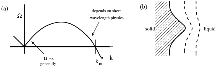
Figure 3: (a) Sketch of the dispersion relation (28) for the stability of the planar solidification interface, in the quasi-stationary approximation. The linear behavior of $\Omega$ with $|k|$ is generic for gradient driven growth problems, while the stabilization for larger $k$ values depends on the problem under consideration. (b) Sketch of the compression of the isotherms in front of a bulge of the interface. If such a bulge appears on a long enough length scale that the capillary suppression of the local melting temperature is not too large, then the enhanced heat diffusion near the bulge associated with the compression of the isotherms makes the interface unstable. This is the origin of the Mullins-Sekerka instability, which is generic to gradient-driven growth problems.

Qualitatively, the origin of the Mullins-Sekerka instability is easy to understand with the help of Fig. 3(b). If the interface has some protrusion into the liquid, then the isotherms are compressed in the neighborhood of this protrusion, provided the length scale of the protrusion is large enough that the suppression of the local melting term due to the capillary correction is small. This means that the heat diffusion away from the interface is enhanced, i.e., that the latent heat produced in this region of the interface diffuses away more easily. Hence the interface can grow faster there, and the protrusion grows larger in time.

It is important to realize that the instability that we identified above only occurs upon growth, and not upon melting if the the heat necessary to melt the crystal is supplied through the melt. This is why ice cubes keep a smooth rounded shape during melting. You are encouraged to repeat the qualitative arguments of Fig. 3(b) to convince yourself of this. See [26] for help and further discussion of this point.

Clearly, the physical mechanism underlying the Mullins-Sekerka instability is not limited to crystal growth: it arises wherenever the growth of or dynamics of a free interface is proportional to the gradient of a field which itself obeys a Laplace equation or diffusion equation — in fact, the approximation $q\approx q^{\prime}\approx k$ that allowed us to reduce the dispersion relation to (28) amounts to replacing the diffusion equation by the Laplace equation in the quasi-stationary limit! Now that we’ve done the analysis once in detail, it is easy to see that the linear dispersion $\Omega\sim|k|$ which we found for solidification for small $k$ [See Fig. 3(a)], is a general feature of diffusion limited or gradient driven interface dynamics. To be specific, consider an interface whose normal velocity $v_{n}$ is propertional to the gradient of some field $\Phi$, which obeys the Laplace equation,

$$v_{n}=\nabla\Phi|_{int}~{},\hskip 42.67912pt\nabla^{2}\Phi=0\hskip 22.76228pt\mbox{in the bulk}~{}.$$ (29)

For a planar solution with velocity $v$, we have then the solution $\Phi_{0}(z)=\Phi^{\prime}_{0}z=vz$. Again, we consider perturbations $\zeta=\zeta e^{\Omega t+ikx}$ of the interface. In order that $\delta\Phi$ then obeys the Laplace equation, it must be of the form

$$\delta\Phi=\delta\Phi_{k}e^{ikx-|k|z}~{},\hskip 42.67912ptz>0~{},$$ (30)

Since to linear order the interface velocity $v_{n}$ in the presence of the perturbation is $v+\dot{\zeta}$, we now have

$$\Omega\zeta_{k}=-|k|\delta\Phi_{k}~{}.$$ (31)

Finally the boundary conditions on the planar interface are such that they can be written in terms of derivatives of the fields or the interface shape, and if the basic equations are translation invariant (i.e., there is no external field that tends to pin the position of the interface), then we must have in linear order

$$\Phi_{0}(\xi_{v}=\zeta_{k})+\delta\Phi_{k}=~{}~{}\mbox{terms of higher order in}~{}k~{},$$ (32)

hence, since $\Phi_{0}^{\prime}=v$,

$$\delta\Phi_{k}=-v\zeta_{k}~{}~{}\mbox{ as }k\rightarrow 0~{}.$$ (33)

Using this in (31), we find

$$\Omega\approx v|k|~{}~{}\mbox{ as }k\rightarrow 0~{}.$$ (34)

This clearly shows the generality of the presence of unstable long wavelength modes with linear dispersion in gradient driven interface dynamics. Not only solidification, but also viscous fingering, streamer formation and flames [7, 8] are subject to this same type of instability, as our discussion earlier in this section demonstrates. The differences between the various problems mainly occur in the stabilizing behavior at short distance scales. These depend on the details of the physics, and are usually different for different problems. They have to be included, however, since otherwise the interface would be completely unstable in the short wavelength limit $k\rightarrow\infty$.

1.5 The connection between viscous fingering and DLA

An interesting illustration of the above observation is given by Diffusion Limited Aggregation (DLA), in which clusters grow due to accretion of brownian particles. Hence the driving force for growth is essentially the same physics as above, a long-range diffusion field governed by the Laplace equation, but in this case there are no stabilizing smoothing terms at shorter wavelength. Only the particle size or the lattice serves as a short distance cutoff, and in this case the growth is fractal [4].

The connection between the viscous fingering problem and DLA is actually quite deep. In the viscous fingering case, the growth is deterministic, and controlled by solving the Laplace equation in the bulk. In DLA, the probability distribution of the random walkers is also governed by the Laplace equation and the flux at the boundary of the growing cluster is proportional to the gradient of the probability distribution of walkers — as we saw, this is the basic ingredient of the Mullins-Sekerka instability. More importantly, however, the DLA growth process is intrinsically noisy as one particle is added at a time, and as there is no relaxation at the boundary of the cluster. As pointed out by Kadanoff et al. [39, 40], the noise can be suppressed by having a cluster grow only at a site once that site has been visited a number of times by a random walker, and by allowing particles at the perimeter to detach and re-attach to the cluster with a probability that depends on the number of neighbors at each site. With increasing noise reduction, DLA in a channel crosses over to viscous fingering.

Another surprising connection is that the mean occupation profile of the average of many realizations of DLA clusters in a channel approaches the shape of a viscous finger. See [41, 42] for details.

2 Smooth fronts as effective interfaces

2.1 Fronts between a stable and a metastable state in one dimension — existence, stability and relaxation

We now turn our attention to a different but related issue, namely the question when we can map a model with a smooth front, domain wall or transition zone, onto a sharp interface model, with boundary conditions which are local in space and time. The answer to this question, namely that this typically can be done for problems in which the interface separates two (meta)stable states or phases may not be that surprising. Nevertheless, thinking about these issues helped us clarify some of the points which we feel have not been paid due attention to in the literature, and which come to the foreground in our work with Ebert and Caroli on streamers [1]. There you really run into trouble if you blindly apply the formalism as it is usually presented in the literature. This will be discussed in detail in our future publications with Ebert [25], and I will keep you in suspense till section 3 for a brief sketch of our present results and implications. Further motivation for the analysis of this section was given in the introduction.

I am convinced most — if not all — elements of the discussion below must appear at many places in the literature. For example, the first part of the analysis appears in one form or another in [12, 13, 14, 15], but since it will arise in almost any Ginzburg-Landau type of analysis — the working horse of condensed matter physics — I presume most ingredients can be found at many more places (similar questions arise in the analysis of instantons in field theory). Nonetheless, we have not come across any discussion from the perspective that we will emphasize in [25], the relation between relaxation, interface limits, and solvability. The present section is intended to provide a summary of the background material that can be found at scattered places in the literature and to serve as an introduction our papers [25].

To be concrete, we will present our discussion in terms of a dynamical equation in one dimension of the form

$${{\partial\phi}\over{\partial t}}={{\partial^{2}\phi}\over{\partial x^{2}}}+g(\phi)~{}.$$ (35)

Here $\phi$ is a real order parameter. This equation is about the simplest model equation for the analysis of relaxation dynamics, but it captures the essentials of the issues that also arise in more complicated variants and extensions.

Later, in our discussion of the coupling to other fields, it is useful to introduce appropriate parameters to tune the time and spatial scales of the variation of $\phi$, but for the present discussion of Eq. (35) we will not need these. We have therefore used the freedom to choose appropriate time and spatial scales to set the prefactors of the derivative terms to unity.

It will turn out to be useful to express $g(\phi)$ in terms of the derivative of two other functions, which both play the role of a potential in different circumstances:

$$g(\phi)\equiv-{{df(\phi)}\over{d\phi}}\equiv{{dV(\phi)}\over{d\phi}}~{},$$ (36)

so that equivalent forms of (35) are

$${{\partial\phi}\over{\partial t}}={{\partial^{2}\phi}\over{\partial x^{2}}}-{{df(\phi)}\over{d\phi}}\hskip 42.67912pt\Longleftrightarrow\hskip 42.67912pt{{\partial\phi}\over{\partial t}}={{\partial^{2}\phi}\over{\partial x^{2}}}+{{dV(\phi)}\over{d\phi}}~{}.$$ (37)

As we shall see later on, $f$ has the interpretation of a free energy density in a Ginzburg-Landau picture, while $V$ will play the role of a particle potential in a standard argument in which there is a one-to-one correspondence between front solutions and trajectories of a particle moving in the potential $V$.

We are interested in cases in which $g(\phi)$ has two zeroes $g(\phi_{s})$ with $g^{\prime}(\phi_{s})<0$; these correspond to (meta)stable homogeneous solutions $\phi=\phi_{s}$ of Eq. (35). Indeed, if we linearize this equation about $\phi_{s}$, and substitute $\Delta\phi\sim e^{\Omega t+ikx}$ (very much like we’ve done before), then we find $\Omega=g^{\prime}(\phi_{s})-k^{2}<0$, which confirms that the state is linearly stable. Without loss of generality, we can always take $g(0)=0$ ($V^{\prime}(0)=0$), so that $\phi=0$ is one of the stable states. We will label the other linearly stable state simply $\phi_{s}$. Although this is not necessary, we will for simplicity also take $g$ antisymmetric [$g(-\phi)=g(\phi)$], so that the potentials $f$ and $V$ are symmetric. A typical example of a function $g(\phi)$ and its corresponding potentials is sketched in Fig. 4. Note that there is also a third root of $g(\phi)$ in between 0 and $\phi_{s}$, and that here $g^{\prime}(\phi_{u})>0$. A homogeneous state $\phi=\phi_{u}$ is therefore unstable ($\Omega=g^{\prime}-k^{2}>0$ for small $k$).

Figure 4: The function $g(\phi)$ and the associated potentials $f(\phi)$ and $V(\phi)$ used in our discussion of front solutions of Eq. (35)

Let us now focuss right away on front or domain wall type solutions of the type sketched in Fig. 5(a): they connect a domain where $\phi\approx\phi_{s}$ on the left to a domain where $\phi\approx 0$ on the right. Obvious questions are: what does the solution look like? In which direction will the front move? And how does it relax to its moving state? The answers to these questions can be obtained in a very appealing and intuitive way for this simple model equation by reformulating the questions into a form that almost every physicist is familiar with. However, the two main points — the existence of a unique solution and exponential relaxation — have more general validity.

We can look for the existence of moving front solutions by making the Ansatz $\phi_{v}(x-vt)=\phi_{v}(\xi_{v})$, with $\xi_{v}=x-vt$. Such solutions are uniformly translating in the $x$ frame, and hence stationary in the co-moving frame $\xi_{v}$. Substitution of this Ansatz into Eq. (37) gives, after a rearrangement

$${{d^{2}\phi_{v}}\over{d\xi_{v}^{2}}}=-v{{d\phi_{v}}\over{d\xi_{v}}}-{{dV(\phi_{v})}\over{d\phi_{v}}}~{}.$$ (38)

This equation is familiar to you: it is formally equivalent to the equation for a “particle” with mass 1 moving in a potential $V$, in the presence of “friction”. In this analogy, which is summarized below, $\xi_{v}$ plays the role of time, and $v$ the role of a friction coefficient:

$$\begin{array}[]{cccc}\xi_{v}&\phi_{v}&v&V\\ \Updownarrow&\Updownarrow&\Updownarrow&\Updownarrow\\ \hskip 11.38092pt\mbox{time}&\hskip 11.38092pt\mbox{displacement}&\hskip 11.38092pt\mbox{friction coefficient}&\hskip 11.38092pt\mbox{potential}\end{array}$$ (39)

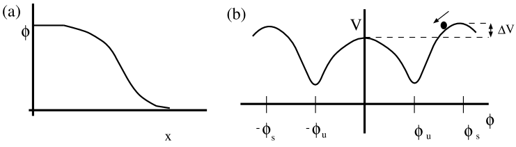
Figure 5: (a) Example of the type of moving front solution we are looking for. (b) The potential $V$. A moving front solution like the one sketched in (a) corresponds in the particle-on-the-hill analogy to the solution of the dynamical problem in which the particle starts at the top at $\phi_{s}$, moves down the hill and up the one in the center, and comes to rest at the center top as the quasi-time $\xi_{v}\rightarrow\infty$.

Clearly, the question whether there is a traveling wave solution of the type sketched in Fig. 5(a) translates into the question, in the particle-on-the-hill analogy: is there a solution in which the particle starts at the top of the potential $V$ at $\phi_{s}$ at “time” $\xi_{v}=-\infty$, rolls down the hill, and comes to rest at the top of the hill at $\phi=0$? In the language of the analogy the answer is immediately obvious: if the value $V(\phi_{s})$ of the potential at $\phi_{s}$ is larger than at $\phi=0$, i.e., if

$$\Delta V\equiv V(\phi_{s})-V(0)$$ (40)

is positive, then there must be a solution with a nonzero positive value of the velocity (the “friction coefficient”). Such a solution corresponds to a front which moves to the right so that the $\phi\approx\phi_{s}$ domain expands. In the opposite case, when the potential at $\phi_{s}$ is lower than at 0 so that $\Delta V<0$, then such a solution only exists for “negative friction” so that enough energy is pumped into the system that the particle can climb the center hill. Negative friction corresponds to a left-moving front with $v<0$, so that the $\phi\approx 0$ domain expands.

Let us make this a bit more precise by first asking what happens when the “friction” $v$ is very large. Then, there is no solution where the particle moves from the top at $\phi_{s}$ to the one at $\phi=0$: for large friction the particle creeps down the hill and comes to rest in the bottom of the potential. When the friction is reduced, the particle looses less energy, and is able to climb further up on the left side of the well. Hence if we keep on reducing the “friction” $v$, at some value $v=v_{0}$ the particle has just enough energy left to climb up all the way to the top at $\phi=0$, and get to rest there. In other words, at $v=v_{0}$, there is a unique solution of the type sketched in Fig. 5(a). If $v$ is reduced slightly below $v_{0}$, the particle overshoots a little bit, and it finally ends up in the left well. So for $v$ just below $v_{0}$, there are no solutions with $\phi_{v}\rightarrow 0$ for $\xi_{v}\rightarrow 0$. However, if we keep on reducing $v$, there comes a point $v=v_{1}$ where the particle first overshoots the middle top, then moves back and forth once in the left well, and finally makes it to the center top — the profile $\phi_{v_{1}}(\xi_{v})$ then has one node where $\phi_{v_{1}}(\xi_{v})=0$. Clearly, we can continue to reduce $v$ and find values $v_{2},v_{3},v_{4},\ldots$ where the profile $\phi_{v_{i}}$ has $2,3,4,\ldots$ nodes. As is illustrated in Fig. 6, we thus have a discrete set of moving front solutions. Which one is stable and dynamically relevant? Intuitively, we may expect that the one with the largest velocity, $v_{0}$, is both the stable and the dynamically relevant one, since the multiple oscillations of the other profiles look rather unphysical. This indeed turns out to be the case: if you start with an initial condition close to the profile $\phi_{v_{1}}$ with velocity $v_{1}$, you will find that the node either “peels off” from the front region and then stays behind, or moves quickly ahead to disappear from the scene on the front end. In both cases, a front with velocity $v_{0}$ emerges after a while. The stability analysis of the front solutions which we will present later confirms that only the fastest $v_{0}$ front solution is linearly stable.

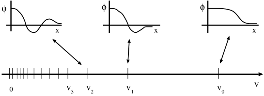
Figure 6: Graphical representation of the fact that a discrete set of moving front solutions is found at velocity values $v_{0},v_{1},v_{2},\ldots$. The number of nodes of the corresponding profiles $\phi_{v_{i}}$ is $i$.

Before turning to the linear stability analysis, we make a brief digression about the connection with a more thermodynamic point of view that is especially popular in studies of coarsening [12, 13, 14, 15].

It is well known that Eqs. (35),(37) can also be written as

$${{\partial\phi}\over{\partial t}}=-{{\delta F}\over{\delta\phi}}~{},\hskip 45.52458ptF=\int dx\left[{\textstyle\frac{1}{2}}\left(\frac{\partial\phi}{\partial x}\right)^{2}+f(\phi)\right]~{}.$$ (41)

In a Ginzburg-Landau like point of view, $F$ plays the role of a free energy functional, whose derivative $\delta F/\delta\phi$ drives the dynamics, and $f(\phi)$ is the coarse grained free energy density. This formulation brings out clearly that the dynamics is relaxational and corresponds to that of a non-conserved order parameter (the conserved case corresponds to $\partial\phi/\partial t=+\nabla^{2}\delta F/\delta\phi$, so that $\int dx~{}\phi$ remains constant under the dynamics). Note also that in statistical physics one often starts with postulating an expression for a coarse grained free energy functional like $F$, and then obtains the dynamics for $\phi$ from the first equation in (41). One should be aware that in pattern formation, one usually has to start from the dynamical equations, and that these usually do not follow from some simple free energy functional [43].

An immediate consequence of (41) is that

$${{dF}\over{dt}}=\int dx~{}{{\delta F}\over{\delta\phi}}{{\partial\phi}\over{\partial t}}=-\int dx\left({{\delta F}\over{\delta\phi}}\right)^{2}\leq 0~{},$$ (42)

so that under the dynamics of $\phi$, $F$ is a non-increasing function of time — it either decreases or stays constant (in technical terms: $F$ is a Lyapunov functional). Since the homogeneous steady states $\phi=0$ and $\phi=\phi_{s}$ correspond to minima of $f(\phi)$ and hence of $F$, this immediately shows that a front moves in the direction so that the domain whose state has the lowest free energy density $f$ expands. Since $f=-V$, this is equivalent to the conclusion reached above, that the domain corresponding to the maximum value of the potential $V$ expands.

Consider now the case in which the states $\phi=0$ and $\phi_{s}$ have the same free energy density: $\Delta f\equiv f(\phi_{s})-f(0)=-\Delta V=0$. They are then “in equilibrium”, and a wall or interface between these two states does not move. Then the excess free energy per unit area, associated with the presence of this wall, which is nothing but the surface tension $\sigma$ is

$$\sigma=\int dx\left[{\textstyle\frac{1}{2}}\left(\frac{\partial\phi_{0}}{\partial x}\right)^{2}+f(\phi_{0})-f(0)\right]~{}.$$ (43)

We can rewrite this by using the fact that energy conservation in the particle picture implies that the sum of the kinetic and “potential” energy ($-f$) is constant, so that ${\textstyle\frac{1}{2}}(\partial\phi_{0}/\partial x)^{2}-f(\phi_{0})=-f(0)$, since far away to the right $\partial\phi_{0}/\partial x\rightarrow 0$ and $\phi_{0}\rightarrow 0$. Using this in (43), we get

$$\sigma=\int dx\left(\frac{\partial\phi_{0}}{\partial x}\right)^{2}~{},$$ (44)

which is an expression which is very often used in square-gradient theories of interfaces. In our case, we can use it to obtain a physically transparant expression for the velocity $v$ of the moving front: If we multiply (38) by $d\phi_{v}/d\xi_{v}$ and integrate over $\xi_{v}$, the term on the left side becomes $\int d\xi_{v}(d\phi_{v}/d\xi_{v})(d^{2}\phi_{v}/d\xi_{v}^{2})$ $={\textstyle\frac{1}{2}}\int d\xi_{v}(\d/d\xi_{v})(d\phi_{v}/d\xi_{v})^{2}=0$ since $d\phi_{v}/d\xi_{v}$ vanishes for $\xi_{v}\rightarrow\pm\infty$. As a result, we are left with

$$v={{\int d\xi_{v}\left[{{d\phi_{v}}\over{d\xi_{v}}}{{df}\over{d\phi}}\right]}\over{\int d\xi_{v}\left({{d\phi_{v}}\over{d\xi_{v}}}\right)^{2}}}={{-\Delta f}\over{\int d\xi_{v}\left({{d\phi_{v}}\over{d\xi_{v}}}\right)^{2}}}~{}.$$ (45)

This expression confirms again that the domain whose state has the lowest free energy $f$ expands. But it shows more: for small differences $\Delta f$, the velocity is small, so we can approximate $\phi_{v}$ in the denominator by $\phi_{0}$, the profile of the interface in equilibrium. But in this approximation, the denominator is nothing but the surface tension of Eq. (44), so

$$v\approx{{-\Delta f}\over{\sigma}}~{},\hskip 42.67912ptv~{}\mbox{small}~{}.$$ (46)

Thus, the response of the interface is linear in the driving force $\Delta f$ and the surface tension $\sigma$ plays the role of an inverse mobility coefficient. The above expressions are often used in the work on coarsening, and can be extended to include perturbatively the effect of curvature or slowly varying additional fields on the interface velocity. We will come to this later.

We now return to the question of stability of the front solutions with velocity $v_{0},v_{1},\ldots$, using an analysis that is inspired by a few simple arguments in [44]. Keep in mind that we will study the stability of front solutions in one dimension themselves, not the stability of a planar interface or front to small changes in its shape, like we did in section 1. To study the linear stability of a front solution $\phi_{v}(\xi_{v})$, we write

$$\phi_{v_{i}}(\xi_{v},t)=\phi_{v_{i}}(\xi_{v})+\eta(\xi_{v},t)~{},$$ (47)

and linearize the dynamical equation (35) in $\eta$ in the moving frame $\xi_{v}$ to get

$${{\partial\eta}\over{\partial t}}=v_{i}{{\partial\eta}\over{\partial\xi_{v}}}+{{\partial^{2}\phi}\over{\partial x^{2}}}+g^{\prime}(\phi_{v_{i}})\eta+O(\eta^{2})~{}.$$ (48)

Since the equation is linear, we can answer the question of stability by studying the spectrum of temporal eigenvalues. To do so, we write

$$\eta(\xi_{v},t)=e^{-Et}e^{-v\xi_{v}/2}\psi_{E}(\xi_{v})~{}.$$ (49)

so that all modes with eigenvalues $E>0$ are stable. Upon substitution of this in (48), we get

$$\begin{array}[t]{r}\left[-{{\partial^{2}}\over{\partial\xi_{v}^{2}}}+\underbrace{\left({{v^{2}}\over{4}}-g^{\prime}(\phi_{v_{i}})\right)}\right]\\ U(\xi_{v})\end{array}\psi_{E}(\xi_{v})=E\psi_{E}(\xi_{v})~{},$$ (50)

which is nothing but the Schrödinger equation (with $\hbar^{2}/m=1$) and which explains why we used $E$ for the temporal eigenvalue in the Ansatz (49). In the analogy with quantum mechanics which we will now exploit, $U(\xi_{v})$ plays the role of a potential , and we are interested in the energy eigenvalues $E$ of the quantum mechanical particle in this potential. If we find a negative eigenvalue, the profile $\phi_{v_{i}}$ is unstable, i.e., there is then at least one eigenmode of the linear evolution operator whose amplitude will grow in time under the dynamics. In other words, if we take as an initial condition for the dynamics the uniformly translating profile $\phi_{v}$ we considered plus a small perturbation about this which has a decomposition along this unstable eigenmode, the perturbation proportional to this eigenmode will grow in time.

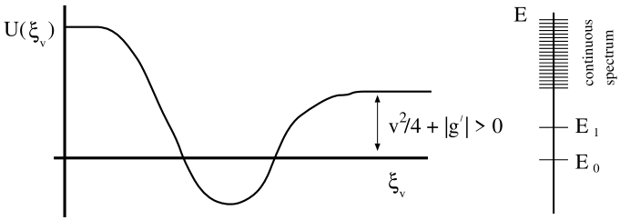
Figure 7: Sketch of the potential $U(\xi_{v})$ which enters in the stability analysis of the front $\phi_{v_{0}}$ between a stable and a meta-stable state. The asymptotes $U(\infty)$ and $U(-\infty)$ are both positive. The resulting eigenvalues spectrum is sketched on the right. Note that there always is an eigenvalue $E=0$ due to the translation mode.

Consider first the form of the potential $U(\xi_{v})$ for $v=v_{0}$. In this case the front has a smooth monotonically decreasing profile of the form sketched in Fig. 5(a). Both for $\xi_{v}\rightarrow-\infty$ and for $\xi_{v}\rightarrow\infty$, $g^{\prime}(\phi_{v_{0}})$ is negative, so $U(\xi_{v})$ is positive for $\xi_{v}\pm\infty$. In between, around $\phi_{v_{0}}=\phi_{u}$, $g^{\prime}(\phi)$ is positive as Fig. 4(a) shows, and so $U(\xi_{v})$ is smaller than its asymptotic values in this range. The resulting shape of $U(\xi_{v})$ is sketched in Fig. 7 for a case in which $U(-\infty)>U(\infty)$. Armed with a physicist’s standard knowledge of quantum mechanics, we can now immediately draw the following conclusions:
          (i) The continuous spectrum corresponds to solutions $\psi_{E}$ that approach plane wave states as $\xi_{v}\rightarrow\infty$ in the case drawn in Fig. 7, and so they have an energy $E\geq U(\infty)=(v_{0}^{2}/4+|g^{\prime}(0)|)>0$. In other words, the bottom of the continuous spectrum lies at a positive energy, and all the corresponding eigenmodes relax exponentially fast.
          (ii) Next, consider the discrete spectrum. Since the original equation is translation invariant, if $\phi_{v_{0}}(\xi_{v})$ is a solution, so is $\phi_{v_{0}}(\xi_{v}+a)=\phi_{v_{0}}(\xi_{v})+a~{}d\phi_{v_{0}}(\xi_{v})/d\xi_{v}+\cdots$. In other words, as the perturbation is nothing but a small shift of the profile, the perturbation should neither grow nor decay. This implies that $d\phi_{v_{0}}(\xi_{v})/d\xi_{v}$ must be a “zero mode” of the linear equation, i.e., be a solution of the Schrödinger equation (49) with eigenvalue $E=0$:

$$E=0:\hskip 28.45274pt\psi_{0}(\xi_{v})={{d\phi_{v_{0}}(\xi_{v})}\over{d\xi_{v}}}~{}.$$ (51)

(iii) Clearly, the “translation mode” $d\phi_{v_{0}}(\xi_{v})/d\xi_{v}$ with eigenvalue zero is a “bound state solution” [as it should, in view of (i)] since it decays exponentially to zero for $\xi_{v}\rightarrow\pm\infty$. Moreover, since $\phi_{v_{0}}$ decays monotonically, $d\phi_{v_{0}}(\xi_{v})/d\xi_{v}<0$, so the translation mode $d\phi_{v_{0}}(\xi_{v})/d\xi_{v}$ does not have a zero, i.e., is nodeless. Now it is a well-known result of quantum mechanics [45] that the bound state wave functions can be ordered according to the number of nodes they have: the ground state with energy $E_{0}$ has no nodes, the first excited bound state (if it exists) has one node, and so on. If we combine this with our observation that $\psi_{0}=d\phi_{v_{0}}(\xi_{v})/d\xi_{v}$ is nodeless and has an eigenvalue $E_{0}=0$, we are led immediately to the conclusion that if there are other bound states, they must have eigenvalues $E>0$.

Taken together, these results show that apart from the trivial translation mode all eigenfunctions have positive eigenvalues $E$ and so are stable: they decay as $t\rightarrow\infty$. Moreover, there is a gap: if the form of the function $g(\phi)$ is such that there are bound state solutions, then the mode that relaxes slowest is the first “excited” bound state solution $\psi_{1}$ with eigenvalue $E_{1}>0$. Otherwise, the slowest relaxation mode is determined by the bottom of the continuous spectrum. In either case, all nontrivial perturbations around the profile $\phi_{v_{0}}$ relax exponentially fast.

It is now easy to extend the analysis to the other front profile solutions $\phi_{v_{1}},\phi_{v_{2}}$, etc. Consider, e.g., $\phi_{v_{1}}$. The analysis of the continuous spectrum proceeds as before so the continuous spectrum again has a gap. Again, the translation mode $d\phi_{v_{1}}(\xi_{v})/d\xi_{v}$ neither grows nor decays, so has eigenvalue zero, but now the fact that $\phi_{v_{1}}$ goes through zero once and then decays to zero implies that $d\phi_{v_{1}}(\xi_{v})/d\xi_{v}$ has exactly one node. According to the connection between the number of nodes of bound state solutions and the ordering of the energy eigenvalues, there must then be precisely one eigenfunction with a smaller eigenvalue than the translation mode which has $E=0$. In other words, there is precisely one unstable mode. Likewise, all other profiles $\phi_{v_{i}}$ with $i\geq 0$ are unstable to $i$ modes.

In summary, our analysis shows that in the dynamical equation (35) for the order parameter $\phi$, there is a discrete set of moving front solutions. Only the fastest one is stable, and its motion is in accord with simple thermodynamic intuition. Moreover, the relaxation towards this unique solution is exponentially fast, as $e^{-\Delta Et}$, where $\Delta E$ is the gap to the lowest bound state eigenvalue, if one exists, or else to the bottom of the continuum band.

2.2 Relaxation and the effective interface approximation

As explained in the introduction, in many cases one wants to map a problem with a smooth but thin front or interfacial zone onto one with a mathematically sharp interface with appropriate boundary conditions. We have termed this the effective interface approximation. Reasons for using this mapping can be either to replace a sharp interface problem by a computationally simpler one with a smooth front (e.g., a so-called phase-field model for a solidification front [5, 6, 46]) or to translate a problem with a thin transition zone (e.g., streamers [1], chemical waves [9, 10], combustion [7, 8]) onto a moving boundary problem, so as to be able to exploit our understanding of this class of problems. We will refer to this literature and to [23] for detailed discussion of the mathematical basis of such approaches. Here, we just want to emphasize how the exponential relaxation of front profiles that we discussed above is a conditio sine qua non for being able to apply this mapping.

For concreteness, let us consider the following phase-field model which is a simple example of the type of models which have been introduced for studying solidification within this context

$$\hskip 73.97733pt{{\partial u}\over{\partial t}} = \nabla^{2}u+{{\partial\phi}\over{\partial t}}~{},$$ (52)

$$\varepsilon{{\partial\phi}\over{\partial t}} = \varepsilon^{2}\nabla^{2}\phi+g(\phi,u)~{},$$ (53)

$$g(\phi,u) = -{{\partial f}\over{\partial\phi}}~{},\hskip 28.45274ptf(\phi,u)=\phi^{2}(\phi-1)^{2}+\lambda u\phi~{}.$$ (54)

In this formulation, $\phi$ is the order parameter field, and $u$ plays the role of a temperature. For fixed $u$, we recognize in (53) the order parameter equation that we have studied before: the potential $f$ has a double well structure for $\lambda u$ small. At $u=0$ the states $\phi=0$ and $\phi=1$ have the same free energy $f$, and the “liquid” state $\phi=0$ and “solid” state $\phi=1$ are then in equilibrium. As we have seen, an interface beween these two states then neither melts nor grows. For $\lambda>0$, a positive temperature $u$ makes the liquid-like state at the minimum near $\phi=0$ the lowest free energy state, and below the melting temperature $u=0$ the solid-like minimum near $\phi=1$ has the lowest free energy. The order parameter equation is coupled to the diffusion equation (52) for the temperature through the term $\partial\phi/\partial t$. This term plays the role of a latent heat term when solidification occurs: it is a source term in the interfacial zone, where $\phi$ rapidly increases from about zero to one. Moreover, if the interface is locally moving with speed $v_{n}$, then $\partial\phi/\partial t\approx-v\partial\phi/\partial\xi_{v}$, so if we integrate through the thin interfacial zone we see that this term contributes a factor $v_{n}$, in agreement with the the fact that the latent heat released at the solid-melt interface is proportional to $v_{n}$.

In writing Eqs. (52)-(54), the space and time scales have been written in units of the “outer” scale on which the temperature field $u$ varies. In these units, the interface width in the order parameter field $\phi$ should be small, and this is why the parameter $\varepsilon\ll 1$ has been introduced in (53): it ensures that the interface width $W$ scales as $\varepsilon$ and that the time scale $\tau$ for the order parameter relaxation is also of order $\varepsilon$. It thus allows us to derive the effective interface equations mathematically using the methods of matched asymptotic expansions or singular perturbation theory [5, 21, 22] by taking the limit $\varepsilon\rightarrow 0$. Since both $W$ and $\tau$ scale as $\varepsilon$ the response of the interface velocity $v_{n}$ stays finite as $\varepsilon$ goes to zero.

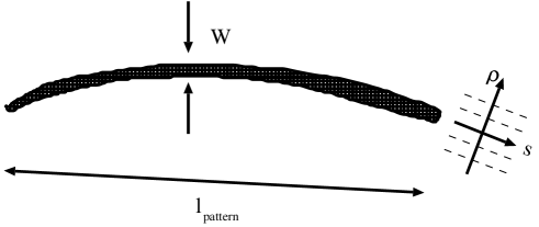
Figure 8: Qualitative sketch of a curved front of width $W$, and the local curvilinear coordinate system $(\rho,{\bf s})$ used in the derivation of an effective interface model.

Although the mathematical analysis by which effective interface equations can be obtained is certainly more sophisticated and systematical than what will transpire from the brief discussion in this section, what seems to be the essential step in all the approaches is the following. In the term $\lambda u$ in $g$ or $f$, which is often treated for convenience as a small perturbation, it is recognized that in the interfacial zone (of width of order $\varepsilon$) $u$ does not change much and hence can effectively be treated as a constant in lowest order. Moreover, since the shape of the interface is curved on the “outer” scale, the curvature $\kappa$ of the interfacial zone, when viewed on the inner scale of the front width, is treated as a small parameter which enters, as we shall see below, the equations in order $\varepsilon$. This is because when $W\rightarrow 0$, the front becomes locally almost planar. As is illustrated in Fig. 8, one now introduces a curved local coordinate system $\rho({\bf r},t),{\bf s({\bf r},t)}$ where the $\rho$ is oriented normal to the front and points in the direction of the $\phi\approx 0$ phase, which in a Ginzburg-Landau description is normally associated with the disordered phase (we thought of it as the “liquid” phase before). By choosing, e.g., the line $\rho=0$ to coincide with the contour line $\phi={\textstyle\frac{1}{2}}$, we ensure that this line follows the interface zone. In the limit $\rho\rightarrow 0$ we then have

$$\lim_{\rho\rightarrow 0}\left.{{\partial\rho}\over{\partial t}}\right|_{\bf r}=-v_{n}({\bf s},t)~{},\hskip 28.45274pt\lim_{\rho\rightarrow 0}\nabla^{2}\rho=\kappa({\bf s},t)~{}.$$ (55)

The derivation of an effective interface approximation now proceeds by introducing the stretched (curvilinear) coordinate $\xi_{v}=\rho/\varepsilon$ for the analysis of the inner structure of the front profile, and assuming that the fields $\phi$ and $u$ can be expanded in a power series of $\varepsilon$ as

$$\mbox{``inner region'':}\hskip 28.45274pt\phi = \phi^{\rm in}_{0}(\xi_{v},{\bf s},t)+\varepsilon\phi^{\rm in}_{1}(\xi_{v},{\bf s},t)+\cdots~{},$$

$$u = u^{\rm in}_{0}(\xi_{v},{\bf s},t)+\varepsilon u^{\rm in}_{1}(\xi_{v},{\bf s},t)+\cdots~{},$$ (56)

$$\mbox{``outer region'':}\hskip 28.45274pt\phi = \phi^{\rm out}_{0}({\bf r},t)+\varepsilon\phi^{\rm out}_{1}({\bf r},t)+\cdots~{},$$

$$u = u^{\rm out}_{0}({\bf r},t)+\varepsilon u^{\rm out}_{1}({\bf r},t)+\cdots~{}.$$ (57)

These “inner” and “outer” expansions then have to obey matching conditions [23, 46] (according to the theory of matched asymptotic expansions [21, 22], the outer expansion of the inner solution has to be equal to the inner expansion of the outer solution). We will not discuss these here, but instead limit ourselves to an analysis of the inner problem. On the inner scale, we have

$$\varepsilon^{2}\nabla^{2}={{\partial^{2}}\over{\partial\xi_{v}^{2}}}+\varepsilon\kappa{{\partial}\over{\partial\xi_{v}}}+O(\varepsilon^{2})~{}.$$ (58)

Furthermore, we shall treat the term $u$ in $g$ formally as a term of order $\varepsilon$ and write $v=v_{1}\varepsilon+\cdots$ and $u=u_{1}\varepsilon+\cdots$ — this is not so elegant and not necessary either, but it gets us to the proper answer efficiently. As the velocity is then also of order $\varepsilon$, this implies that $\phi_{0}$ is then the stationary front profile ($\partial\phi_{0}/\partial\xi_{v}=0$) between two phases in equilibrium, so that from (54) the lowest order equation becomes

$${{\partial^{2}\phi^{\rm in}_{0}}(\xi_{v})\over{\partial\xi_{v}^{2}}}+g(\phi^{\rm in}_{0}(\xi_{v}),0)=0~{}.$$ (59)

The solution of this equation is just the equilibrium profile $\phi_{0}$ that we introduced in our discussion of the surface tension. Of course, it is not at all surprising that (59) emerges in lowest order, since at $u=0$ the two phases are in equilibrium. Now, in the next order, we get

$$\left({{\partial^{2}}\over{\partial\xi_{v}^{2}}}+g^{\prime}(\phi^{\rm in}_{0})\right)\phi^{\rm in}_{1}(\xi_{v})=-(v_{1}+\kappa){{\partial\phi^{\rm in}_{0}(\xi_{v})}\over{\partial\xi_{v}}}-\left.{{\partial g(\phi^{\rm in}_{0},u)}\over{\partial u}}\right|_{u=0}u_{1}~{}.$$ (60)

This equation allows us to solve for $\phi^{\rm in}_{1}$ in principle. But even without doing so explicitly, we can get the most important information out of it. The operator between parentheses on the left is nothing but the linear operator we already encountered before: the Schrödinger operator in our discussion of stability. We then saw that this operator has a mode with eigenvalue zero, the translation mode $\d\phi_{0}/d\xi_{v}$. Moreover, since the operator is hermitian, it is also a left eigenmode with eigenvalue zero of this operator. This implies that for the equation to be solvable, the right hand side has to be orthogonal to the left zero mode $\d\phi_{0}/d\xi_{v}$. This conditions leads to a so-called solvability condition. Upon multiplying Eq. (60) by $\d\phi_{0}/d\xi_{v}$ and integrating, we can write this condition as an expression for the normal interface velocity $v_{n}$ to lowest order in $\varepsilon$,

$$v_{n}=-\kappa-{{\int d\xi_{v}{{d\phi_{0}}\over{d\xi_{v}}}{{\partial g(\phi_{0},u)}\over{\partial u}}~{}u_{1}}\over{\int d\xi_{v}\left({{d\phi_{0}}\over{d\xi_{v}}}\right)^{2}}}~{}.$$ (61)

Here, we used the fact that $\phi^{\rm in}_{0}=\phi_{0}$. Moreover, in the integration on the right hand side, we can take $u$ constant, since the temperature does not vary to lowest order in the interfacial region (its derivatives do — see [46] for more details).

The above expression is our central result. The fact that the prefactor of the curvature term on the right is unity comes from the fact that the curvature enters according to the expansion (58) of the diffusion term $\nabla^{2}$ in precisely the same way as the velocity term that arises from the transformation to the co-moving curvilinear from $\xi_{v}$. When $u_{1}=0$, i.e., when we consider an interface between two equilibrium phases, it expresses the tendency of the interfaces to straighten out. This effect drives coarsening [12, 13, 14, 15], and the motion is sometimes refered to as motion by mean curvature. The second term gives the driving term when the interface temperature $u$ is not equal to the equilibrium temperature. The structure of this term is also quite transparent. In the denominator, we recognize the surface tension (44), and as we already discussed, the inverse of the surface tension plays the role of an interface mobility in the context of the type of models we consider. In the numerator we can write $g$ in terms of $-\partial f(\phi_{0},u)/\partial\phi_{0}$ and then do the integral in the same way as before in deriving (45); we then simply get

$$v_{n}=-\kappa-{{1}\over{\sigma}}\left.{{d\Delta f}\over{du}}\right|_{u=0}u~{}.$$ (62)

where now $\Delta f$ is the difference in free energy densities at opposite sides of the interface. Clearly, the second term is exactly what we could have guessed on the basis of what we already knew before, and together with the curvature term it has exactly the same type of structure as the boundary condition (3) that we introduced in our first discussion of solidification. The complications that are necessary to model anisotropic kinetics and surface tension with a phase-field model are significant [6], but conceptually the analysis is essentially the same.

By taking big steps, we have not done justice to the systematics of the analysis, and there is much more to say about it. If you want to know more, you will find entries to the literature in [5, 6, 23, 46]. However, the point we want to bring to the foreground, following [25] is that in all such approaches, a hidden assumption is made in writing the inner expansion as $\phi^{\rm in}=\phi^{\rm in}_{0}(\rho/\varepsilon,{\bf s},t)+\cdots$ in (56). In doing so, we basically already assume that on the slow time scale $t$, the profile responds instantaneously to variations in the outer field $u$. This is why on the inner scale, the changes in the profile (like $\phi^{\rm in}_{1}$) are given by ordinary differential equations with coefficients which may vary on the outer slow time scale. As it happens, this is actually justified for these type of problems. For, we have seen that the relaxation of a profile goes exponentially fast, as the spectrum of temporal eigenvalues $E$ has a finite gap $\Delta E$. In the present case, where the time scale $\tau$ in the order parameter equation scales as $\varepsilon$, this means that the relaxation of the front profile goes as $e^{-\Delta Et/\varepsilon}$. This shows that as $\varepsilon\rightarrow 0$, the adiabatic assumption implicit in the above analysis is right, as the relaxation on the inner scale completely decouples from the slow scale variation of the outer fields. In other words: we have left out exponentially small terms as $\varepsilon\rightarrow 0$, but that is something that almost always happens when we an asymptotic expansion! As we shall see now, the adiabatic approximation can not be made for fronts moving into an unstable state, such as streamers.

3 Some elements of front propagation into unstable states — relaxation and the effective interface approximation

We now briefly touch on a few elements of fronts propagating into unstable states. In view of the length restrictions on the contribution to the proceedings of the school, we only highlight some recent results obtained in collaboration with Ebert [25], which show that a large class of fronts propagating into an unstable state show universal power law relaxation and that this makes the mapping of such fronts onto an effective interface model questionable.

Our own motivation comes from our attempt to understand the streamer problem, but examples of fronts propagating into an unstable state arise in various fields of physics: they are important in many convective instabilities in fluid dynamics such as the onset of von Karman vortex generation [52], in Taylor [53] and Rayleigh-Bénard [19] convection, they play a role in spinodal decomposition near a wall [54], the pearling instability of laser-tweezed membranes [55], the formation of kinetic, transient microstructures in structural phase transitions [56], the propagation of a superconducting front into an unstable normal metal [57], or in error propagation in extended chaotic systems [58]. The experimental relevance of the understanding of the relaxation of such fronts is illustrated on propagating Taylor vortex fronts. Here the measured velocities were about 40% lower than predicted theoretically [53], and only later numerical simulations [59] showed that this was due to slow transients.

When one of the states is unstable, even a small perturbation around this state will grow out and spread; therefore, the properties of fronts that propagate into an unstable state depend on the initial conditions. If the initial profile is steep enough, arising, e.g., through local initial perturbations, it is known that the propagating front in practice always relaxes to a unique profile and velocity [47, 44, 48, 49, 51]. Depending on the nonlinearities, one generally can distinguish two regimes: as a rule, fronts whose propagation is driven (“pushed”) by the nonlinearities, resemble very much the fronts which propagate into a metastable state and which we have discussed extensively in section 2 (e.g., their relaxation is also exponential in time). We will therefore not consider this regime, which is often refered to as “pushed” [50, 51] or “nonlinear marginal stability” [49] any further. If, on the other hand, nonlinearities mainly cause saturation, fronts propagate with a velocity determined by linearization about the unstable state, as if they are “pulled” by the linear stability (“pulled” [50, 51] or “linear marginal stability” [48, 49] regime).

Almost all important differences between “pulled” or “linear marginal stability” fronts propagating into an unstable state and those propagating into a metastable state trace back to the fact that in the latter case there typically is a discrete set of front solutions, only one of which is stable as was illustrated in Fig. 6, while in the former case there generally is a family of moving front solutions [47, 44, 48, 49]. To illustrate this, we again turn to Eq. (35), but now take $g(\phi)$ of the form sketched in Fig. 9(a). In this case, $g^{\prime}(0)>0$, so the state $\phi=0$ is unstable. If we again consider fronts propagating into this state, the potential $V$ corresponding to this function $g$ is the one shown in Fig. 9(b). Now, the question of the existence of a uniformly translating profile $\phi_{v}(x-vt)=\phi(\xi_{v})$ translates into the question “is there a solution in the particle on the hill analogy in which the particle starts at time $\xi_{v}=-\infty$ at the top, and comes to the bottom as $\xi_{v}\rightarrow\infty$?”. Obviously, there is such a solution for any positive value of the “friction coefficient” $v$: there is a continuous family of uniformly translating front solutions.

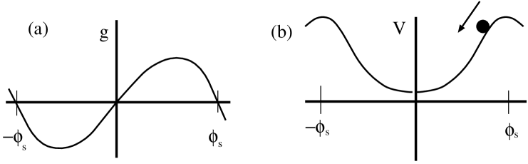
Figure 9: The functions $g$ and $V$ in the case of front propagation into unstable states. Compare Fig. 4, where the functions are drawn for the case of a front between a stable and a metastable state.

It is useful to consider the relation between the velocity $v$ which labels the front solutions, and the asymptotic decay rate $\Lambda$: if we linearize Eq. (35) around the state $\phi=0$ and write $\phi_{v}\sim e^{-\Lambda\xi_{v}}$, then we get $v\Lambda=\Lambda^{2}+g^{\prime}(0)$, so

$$\Lambda_{\pm}={{v}\over{2}}\pm\sqrt{{{v^{2}}\over{4}}-g^{\prime}(0)}~{},\hskip 42.67912ptg^{\prime}(0)>0~{}.$$ (63)

For $v>2g^{\prime}(0)$, the roots are real, and $\Lambda_{-}<\Lambda_{+}$. For $v<2g^{\prime}(0)$, the roots are complex, meaning that the front solutions decay to zero as $\phi_{v}\sim\cos(\Im\Lambda_{\pm}\xi_{v})e^{-\Re\Lambda_{\pm}\xi_{v}}$. Clearly, the velocity $v^{*}=2g^{\prime}(0)$ is a special value, as the two roots coincide there $\Lambda_{-}=\Lambda_{+}=\Lambda^{*}$. It is a well-known result that in such a degenerate case, the front profile does not decay as a single exponential, but that instead in this case

$$\phi_{v^{*}}(\xi_{v})\sim(\xi_{v}+\mbox{const.})e^{-\Lambda^{*}\xi_{v}}~{}.$$ (64)

so that the dominant behavior for large $\xi_{v}$ is the $\xi_{v}e^{-\Lambda^{*}\xi_{v}}$ term.

The special status of the value $v^{*}$ also becomes clear when we look at the stability analysis of the fronts $\phi_{v}(\xi_{v})$. If we retrace the stability analysis of section 2, then in this case the potential $U(\xi_{v})$ in the Schrödinger type equation for the spectrum has an asymptotic value $(v^{*})^{2}/4-g^{\prime}(0)=0$. Hence, according to our arguments the continous spectrum associated with quantum mechanically allowable eigenfunctions $\psi$ comes all the way down to zero, i.e., there is no gap. This already gives a hint that there will be non-exponential relaxation.

In the derivation of effective interface equations, we encountered solvability conditions which involved integrals of the form $\int dx(d\phi_{0}/dx)^{2}$ — see Eq. (61). In the present case, the front velocity is always nonzero, and as a result the stability operator is non-hermitian [25]. If one tries to derive effective interface equations for such fronts using the same type of approach as discussed at the end of section 2, one needs the zero mode of the adjoint operator of the problem with $v\neq 0$ in the corresponding solvability condition. Because of the non-hermitian nature of this operator for $v\neq 0$, this zero mode turns out to be $e^{v\xi_{v}}(\d\phi_{v}/d\xi_{v})$, and one encounters integrals of the type $\int d\xi_{v}e^{v\xi_{v}}(d\phi_{v}/d\xi_{v})^{2}$ (note that for $v=0$, the zero mode of the adjoint operator reduces to the one we used before, $\partial\phi_{0}/\partial\xi_{v}$). As $\xi_{v}\rightarrow\infty$, the integrand behaves as $e^{(v-2\Lambda_{-})\xi_{v}}=e^{\sqrt{v^{2}/4-g^{\prime}(0)}\xi_{v}}$. As a result, the integrals that arise if one naievely applies the standard analysis do not converge. Although there have been some suggestions [61] that one might regularize such integrals by introducing a cutoff which is taken to infinity at the end of the calculations, such fixes do not appear to work here and obscure the connection of this problem with the slow relaxation discussed below.

We have not yet discussed the origin of the result that “pulled” fronts which emerge from sufficiently localized initial conditions move with a speed $v^{*}$ determined by the linear behavior of the dynamical equation [in our case, the fact that $v^{*}$ is determined solely by $g^{\prime}(0)$]. The origin lies in the fact that any perturbation about the unstable state grows out and spreads by itself. This leads to a natural spreading speed of linear perturbations, and $v^{*}$ is nothing but this speed itself [49, 60]. If nonlinearities mainly suppress further growth, then indeed the dynamically relevant front is “pulled” [50] by the leading edge whose dynamics is governed by the linearized equation. Ebert and I have recently found that one can build on this idea to analyze the relaxation of front profiles towards $\phi_{v^{*}}$ [25]. The main idea can be illustrated within the context of the dynamical equation (35) as follows. Let us use the freedom of choosing appropriate space and time scales to take $g^{\prime}(0)=1$. As the discussion following Eq. (63) shows, $v^{*}=2$ and $\Lambda^{*}=1$ in this case, and the linearized dynamical equation reads

$${{\partial\phi(x,t)}\over{\partial t}}={{\partial^{2}\phi(x,t)}\over{\partial x^{2}}}+\phi(x,t)~{}.$$ (65)

We now write the equation in the moving frame $\xi_{v}=x-v^{*}t$ moving with velocity $v^{*}=2$, and make the transformation $\phi(\xi_{v},t)=e^{-\xi_{v}}\psi(\xi_{v},t)$. This is essentially the same type of transformation that we did before in (49) when we performed the stability analysis of moving front solutions. With these transformations, $\psi$ simply obeys the diffusion equation

$${{\partial\psi(\xi_{v},t)}\over{\partial t}}={{\partial^{2}\psi(\xi_{v},t)}\over{\partial x^{2}}}~{}.$$ (66)

As is well known, in many diffusion type problems the long time asymptotics is governed by the fundamental similarity solution or one of its derivatives, like

$$\psi^{\rm sym}_{1}={{1}\over{{t}^{1/2}}}e^{-\xi_{v}^{2}/4t}~{},\hskip 14.22636pt\mbox{or}\hskip 14.22636pt\psi^{\rm sym}_{2}=-{{\partial\psi^{\rm sym}_{1}}\over{\partial\xi_{v}}}={{\xi_{v}}\over{2\ t^{3/2}}}e^{-\xi_{v}^{2}/4t}~{},$$ (67)

so it is not unreasonable to expect that one of these similarity solutions also governs the long time asymptotics in the leading edge here. If so, the corresponding function $\phi(\xi_{v},t)$ should approach the dominant $\xi_{v}e^{-\xi_{v}}$ term of (64) for large times. As $\psi=e^{\Lambda^{*}\xi_{v}}\phi$, this means that the spatial dependence of the similarity solution $\psi^{\rm sym}$ that we are looking for should go as $\xi_{v}$ for $\xi_{v}^{2}\ll t$. Clearly, the appropriate one is $\psi^{\rm sym}_{2}$. Hence, this simple argument suggests that in the frame moving with velocity $v^{*}=2$, the dominant long time dynamics in the leading edge is

$$\phi\sim{{\xi_{v}}\over{t^{3/2}}}e^{-\xi_{v}-\xi_{v}^{2}/4t}=e^{-\xi_{v}-3/2\ln t+\ln\xi_{v}-\xi_{v}^{2}/4t}~{}.$$ (68)

If we now track the position $\xi_{h}(t)$ of the point where $\phi(\xi_{v},t)=h$, we get to dominant order from the requirement that the exponent in the above expression remains constant

$$\xi_{h}=-{{3}\over{2}}\ln t+\cdots\hskip 28.45274pt\Longleftrightarrow\hskip 28.45274pt\dot{\xi}_{h}=-{{3}\over{2t}}+\cdots$$ (69)

As $\dot{\xi}_{h}$ is the velocity of the point where $\phi=h$, we see that in the leading edge of the profile the velocity relaxes towards $v^{*}$ as $-3/(2t)$. This is precisely what was found by Bramson [62] from a rigorous analysis. Although the above argument is rather handwaving, we have recently found [25] that it can be made into a systematic asymptotic analysis which applies not just to the second order dynamical equation (35), but also to higher order partial differential equations which admit uniformly translating front solutions. The surprising finding is that not just the leading order $\sim 1/t$ relaxation term in the velocity is universal, but also the first subdominant $\sim 1/t^{3/2}$ term, which can not be obtained from the sove argument: independent of the “height” $h$ whose position we track, we find that the velocity $v_{h}(t)=v^{*}+\dot{\xi}_{h}$ relaxes to $v^{*}$ as

$$v_{h}=v^{*}-{{3}\over{2\Lambda^{*}t}}\left(1-\frac{\sqrt{\pi}}{\Lambda^{*}\sqrt{Dt}}\right)+O\left(\frac{1}{t^{2}}\right)~{},$$ (70)

where for the order parameter equation (35) with $g^{\prime}(0)=1$, $v^{*}=2$, $\Lambda^{*}=1$ and $D=1$. In the more general case, $D$ is a coefficient which plays the role of a diffusion coefficient, and which can be determined explicitly from the dispersion relation of the linearized equation. Moreover, also the shape of the profile relaxes with the same slow power laws in a universal way which is related to the existence of a family of front solutions. We refer to [25] for details.

The above $1/t$ power law relaxation is clearly too slow to make an effective interface approximation with boundary conditions which are local in space and time possible for “pulled” fronts whose propagation into an unstable states originates in diffusive spreading and growth. To see this, consider, e.g., a spherically symmetric front in Eq. (35) in three dimensions which grows out from some localized region around the origin. For long times the front region is thin in comparison with the distance $r_{f}$ from the origin and the curvature of the front is small and of order $2/r_{f}\approx 2/(2v^{*}t)$. Thus, the curvature is of the same order as the dominant relaxation term of the front, and one can not simply express the instantaneous front velocity in terms of $v^{*}$ plus some kind of curvature correction, as we saw one can do for fronts between a stable and a metastable state. Some preliminary numerical investigations have confirmed this. Whether some other interfacial description with memory type of terms can be developed, or whether there are other unexpected consequences of this slow relaxation, is at present an open question.

References

- [1] U. Ebert, W. van Saarloos and C. Caroli, Streamer formation as a Pattern Formation Problem: Planar Fronts , Phys. Rev. Lett. 77, 4178 (1996); Propagation and structure of planar streamer fronts, Phys. Rev. E 55, 1530 (1997).
- [2] E. Brener, H. Müller-Krumbhaar and D. Temkin, Structure formation and the morphology diagram of possible structures in two-dimensional diffusional growth, Phys. Rev. E 54, 2714 (1996).
- [3] W. W. Mullins and R. F. Sekerka, Morphological stability of a particle growing by diffusion or heat flow, J. Appl. Phys. 34 323 (1963); Stability of a planar interface during solidification of a dilute binary alloy, J. Appl. Phys. 35, 444 (1964).
- [4] P. Meakin, The growth of Fractal aggregates and their fractal measures, in: Phase transitions and critical phenomena, ed. C. Domb and J. L. Lebowitz, vol. 12 (Academic, New York, 1988).
- [5] The literature on phase-field models is vast by now. An entry into the more mathematically oriented literature can be got from P. W. Bates, P. C. Fife, R. A. Gardner and C. K. R. T. Jones, Phase-field Models for Hypercooled Solidification, Physica D 104, 1 (1997).
- [6] An example where a phase-field model has been exploited numerically to study the dendrite problem is A. Karma, W.-J. Rappel, Phase-field method for computationally efficient modelling of solidification with arbitrary interface kinetics Phys. Rev. E 53, R3017 (1996), and Quantitative phase-field modeling of dendritic growth in two and three dimensions (preprint, July 1997). These papesr also give an entry to the more physics oriented literature. An early use of the word “phase-field model” is found in the article Models of pattern formation in first order phase transitions, by J. S. Langer, in: Directions in Condensed Matter Physics, G. Grinstein and G. Mazenko, eds. (World Scientific, Singapore, 1986).
- [7] J. D. Buckmaster and G. S. S. Lundford, Theory of Laminar Flames, (Cambridge University Press, Cambridge, 1982).
- [8] A very nice elementary account of several of the essential ingredients of flame fronts and their instabilities can be found in J. D. Buckmaster, Fronts and patterns in low Mach No. combustion — a review, Physica 12D, 173 (1984).
- [9] See, e.g., E. Meron, Pattern Formation in Excitable Media, Phys. Rep. 218, 1 (1992).
- [10] R. E. Goldstein, D. J. Muraki and D. M. Petrich, Interface proliferation and the growth of labyrinths in a reaction-diffusion system, Phys. Rev. E 53, 3933 (1996).
- [11] M. Kléman, Points, Lines and Walls in Liquid Crystals, Magnetic Systems and Various Ordered Media (Wiley, 1983 New York).
- [12] J. D. Gunton, M. San Miguel and P. S. Sahni, The dynamics of First Order Phase Transitions, in: Phase Transitions and Critical Phenomena, Vol. 8, ed. C. Domb and J. L. Lebowitz (Adademic, New York, 1983).
- [13] A. J. Bray, Theory of Phase Ordering Kinetics, Adv. Phys. 43, 357 (1994).
- [14] J. S. Langer, An introduction to the kinetics of first-order phase transition, in: Solids far from Equilibrium, C. Godreche, Ed. (Cambridge University Press, Cambridge, 1992)
- [15] Here, smooth interface models go back to the classic work of S. M. Allen and J. W. Cahn, A microscopic theory for antiphase boundary motion and its application to antiphase domain coarsening, Acta Metall. 27, 1085 (1979).
- [16] P. C. Hohenberg and B. I. Halperin, Theory of dynamic critical phenomena Rev. Mod. Phys. 49, 435 (1977).
- [17] M. C. Cross and P. C. Hohenberg, Pattern formation outside of equilibrium, Rev. Mod. Phys. 65, 851 (1993).
- [18] See M. A. Anisimov, P. E. Cladis, E. E. Gorodetskii, D. A. Huse, V. E. Podneks, V. G. Taratuta, W. van Saarloos and V. P. Voronov, Experimental Test of a Fluctuation Induced First Order Transition: the Nematic-Smectic A Transition, Phys. Rev. A 41, 6749 (1990), and references therein.
- [19] J. Fineberg and V. Steinberg, Vortex front propagation in Rayleigh Benard convection, Phys. Rev. Lett. 58, 1332 (1987).
- [20] M. P. M. den Nijs, The domain wall theory of two-dimensional commensurate-incommensurate phase transitions, in: Phase transitions and critical phenomena, ed. C. Domb and J. L. Lebowitz, vol. 12 (Academic, New York, 1988).
- [21] C. M. Bender and S. A. Orszag, Advanced Mathematical Methods for Scientists and Engineers (McGraw-Hill, New York, 1978).
- [22] M. Van Dyke, Perturbation methods in Fluid Mechanics (Parabolic Press, Stanford, 1975).
- [23] P. C. Fife, Dynamics of Internal Layers and Diffusive Interfaces (SIAM, Philadelphia, 1988).
- [24] For an overview of adiabatic decoupling in ordinary differential equations as a result of the separation of time scales, see e.g., N. G. van Kampen Elimination of fast variables, Phys. Rep. 124, 69 (1985).
- [25] U. Ebert and W. van Saarloos, Universal algebraic relaxation of fronts propagating into an unstable state and implications for moving boundary approximations, scheduled to appear in the Feb. 23 1998 issue of Phys. Rev. Lett. (for an earlier version, see http://xxx.lanl.gov/abs/patt-sol/9707004); a longer version of this article is in preparation.
- [26] J. S. Langer, Instabilities and Pattern Formation in Crystal Growth, Rev. Mod. Phys. 52, 1 (1980); in Chance and Matter, ed. J. Souletie (North-Holland, Amsterdam, 1987).
- [27] B. Caroli, C. Caroli and B. Roulet, Instabilities of planar solidification fronts, in: Solids far from Equilibrium, ed. G. Godrèche (Cambridge University Press, Cambridge, 1992)
- [28] K. Kassner, Pattern Formation in Diffusion-Limited Crystal Growth (World Scientific, Singapore, 1996).
- [29] For a review of the issues related to the microscopic nature of the crystal-melt interface, see, e.g., J. D. Weeks, The roughening transition, in: Ordering in strongly fluctuating condensed matter systems, ed. T. Riste (Plenum, New York, 1980), or P. Nozières, Shape and Growth of Crystals in: Solids far from Equilibrium, ed. G. Godrèche (Cambridge University Press, Cambridge, 1992).
- [30] E. Rolley, S. Balibar and F. Graner, Growth shapes of needle crystals, Phys. Rev. E 49, 1500 (1994).
- [31] P. Tabeling, G. Zocchi and A. Libchaber, An experimental study of the Saffman-Taylor instability, J. Fluid Mech. 177, 67 (1987).
- [32] P. A. Vitello, B. M. Penetrante and J. N. Bardsley, Simulation of negative-streamer dynamics in nitrogen, Phys. Rev. E 49, 5574 (1994).
- [33] P. A. Vitello, B. M. Penetrante and J. N. Bardsley, Multi-dimensional modeling of the dynamic morphology of streamer coronas, in: Non-Thermal Plasma Techniques for Pollution Control, eds. B. M. Penetrante and S. E. Schultheis (Springer, Berlin, 1993).
- [34] D.A. Kessler, J. Koplik and H. Levine, Pattern selection in fingered growth phenomena, Adv. Physics 37, 255 (1988); P. Pelcé, Dynamics of Curved Fronts (Academic, Boston, 1988); and Y. Pomeau and M. Ben Amar, Dendritic growth and related topics, in: Solids far from Equilibrium, C. Godreche, Ed. (Cambridge University Press, Cambridge, 1992); E. A. Brener and V. I. Mel’nikov, Pattern selection in two-dimensional dendritic growth, Adv. Phys. 40, 53 (1991).
- [35] For this reason, kinetic relations like (3) can easily be studied with computer simulations. For an example of this, see, e.g., J. Q. Broughton, G. H. Gilmer and K. A. Jackson, Crystallization rates of a Lennard-Jones liquid, Phys. Rev. Lett. 49, 1496 (1982). The interface mobility coefficient in (3) is nothing but the slope of Fig. 3 in this paper.
- [36] E. Brener, Needle-crystal solution in three-dimensional dendritic growth, Phys. Rev. Lett. 71, 3653 (1993).
- [37] D. Bonn, H. Kellay, M. Ben Amar and J. Meunier, Viscous finger widening with surfactants and polymers, Phys. Rev. Lett. 75, 2132 (1995).
- [38] L. Puech, G. Bonfait and B. Castaing, Polarized : dendritic melting, J. Physique 47, 723 (1986).
- [39] L. P. Kadanoff, Simulating hydrodynamics: a pedestrian model, J. Stat. Phys. 39, 267 (1985).
- [40] D. Bensimon, L. P. Kadanoff, S. Liang, B. I. Shraiman, C. Tang Viscous flow in two dimensions, Rev. Mod. Phys. 58, 977 (1986).
- [41] A. Arneodo, Y. Couder, G. Grasseau, V. Hakim and M. Rabaud, Pattern growth: from smooth interfaces to fractal structures, in: Nonlinear evolution of spatio-temporal structures in dissipative continuous systems, F. H. Busse and L. Kramer, ed. (Plenum, New York, 1990).
- [42] E. Brener, H. Levine and Y. Tu, Mean-field theory for Diffusion-Limitied Aggregation in Low dimensions, Phys. Rev. Lett. 66, 1978 (1991).
- [43] A very enjoyable article which discusses fronts in various non-gradient systems is M. San Miguel, R. Montagne, A. Amengual and E. Hernández-García, Multiple front propagation in a potential non-gradient system, in: Instabilities in Nonequilibrium structures V, eds. E. Tirapegui and W. Zeller (Kluwer, Dordrecht, 1996).
- [44] E. Ben-Jacob, H. R. Brand, G. Dee, L. Kramer and J. S. Langer, Pattern propagation in non-linear dissipative systems, Physica D 14, 348 (1985).
- [45] A. Messiah, Quantum Mechanics (North-Holland, Amsterdam, 1974).
- [46] R. Kupferman, O. Shochet, E. Ben-Jacob and A. Schuss, Phase-field model: boundary layer, velocity of propagation, and the stability spectrum, Phys. Rev. B 46, 16045 (1992).
- [47] D. G. Aronson, and H. F. Weinberger, Multidimensional nonlinear diffusion arising in population dynamics, Adv. Math. 30, 33 (1978).
- [48] W. van Saarloos, Front propagation into unstable states: Marginal stability as a dynamical mechanism for velocity selection, Phys. Rev. 37, 211 (1988).
- [49] W. van Saarloos, Front propagation into unstable states. II Linear versus nonlinear marginal stability and rate of convergence, Phys. Rev. A 39, 6367 (1989).
- [50] The terms pulled and pushed were introduced by A. N. Stokes, On two types of moving front in Quasilinear diffusion, Math. Biosc. 31, 307 (1976).
- [51] G. C. Paquette and Y. Oono, Structural stability and selection of propagating fronts in semi-linear parabolic partial differential equations, Phys. Rev. E 49, 2368 (1994); G. C. Paquette, L.-Y. Chen, N. Goldenfeld and Y. Oono, Structural stability and renormalization group for propagating fronts, Phys. Rev. Lett. 72, 76 (1994).
- [52] C. Mathis, M. Provansal and L. Boyer, The Benard-Von Karman instability: an experimental study near threshold, J. Phys. Lett. 45, L483 (1984); G.S. Triantafyllou, K. Kupfer and A. Bers, Absolute instabilities and self-sustained oscillations in the wakes of circular cylinders, Phys. Rev. Lett. 59, 1914 (1987).
- [53] G. Ahlers and D. S. Cannell, Vortex front propagation in rotating Couette-Taylor flow, Phys. Rev. Lett. 50, 1583 (1983).
- [54] R. C. Ball, R. L H. Essery, Spinodal decomposition and pattern formation near surfaces, J. Phys.: Condens. Matter 2, 10303 (1990); R. A. L. Jones, L.J. Norton, E. J. Kramer, F. S. Bates, P. Wiltzius, Surface-directed spinodal decomposition, Phys. Rev. Lett. 66, 1326 (1991).
- [55] T. R. Powers and R. E. Goldstein, Pearling and pinching: propagation of Rayleigh instabilities, Phys. Rev. Lett. 78, 2555 (1997); see also L. Limat, P. Jenffer, B. Dagens, E. Touron, M. Fermigier, J. E. Wesfreid Gravitational instabilities of thin liquid layers: dynamics of pattern selection, Physica D 61, 166 (1992).
- [56] E. K. H. Salje, On the kinetics of partially conserved order parameters: a possible mechanism for pattern formation, J. Phys.: Condens. Matter 5, 4775 (1993).
- [57] S. J. Di Bartolo, A. T. Dorsey, Velocity selection for propagating fronts in superconductors, Phys. Rev. Lett. 77, 4442 (1996), and references therein.
- [58] A. Torcini, P. Grassberger, A. Politi, Error propagation in extended chaotic systems, J. Phys. A 27, 4533 (1995).
- [59] M. Niklas, M. Lücke and H. Müller-Krumbhaar, Velocity of a propagating Taylor-vortex front, Phys. Rev. A 40 493 (1989).
- [60] L. D. Landau and E. M. Lifshitz, Course of Theoretical Physics, vol. 10 (Pergamon, New York, 1981).
- [61] L.-Y. Chen, N. Goldenfeld, Y. Oono and G. Paquette, Selection, stability and renormalization, Physica A 204, 111 (1994).
- [62] M. Bramson, Convergence of solutions of the Kolmogorov equation to traveling waves, Mem. Am. Math. Soc. 44, No. 285 (1983).