Thermal Fluctuations, Subcritical Bifurcation, and Nucleation of Localized States in Electroconvection

Abstract

Measurements of the mean-square amplitude $\langle\theta^{2}\rangle$ of thermally-induced fluctuations of a thin layer of the nematic liquid crystal I52 subjected to a voltage $V<V_{c}$ are reported. They yield the limit of stability $V_{c}$ of the spatially uniform conduction state to infinitesimal perturbations. Localized long-lived convecting structures known as worms form spontaneously from the fluctuations for $V$ well below $V_{c}$. This, as well as measurements of the lifetime of the conduction state for $V<V_{c}$, suggests a thermally-activated mechanism of worm formation; but a theory for this non-potential system is lacking.

One of the uniquely nonlinear aspects of pattern-forming dissipative non-equilibrium systems is the occurrence of localized travelling-wave structures, or pulses, co-existing with the spatially uniform ground state.[1] In one-dimensional cases[2, 3] it has been possible to understand such structures qualitatively in terms of a subcritical Ginzburg-Landau equation [4]; but for systems which are spatially extended in two dimensions [5] theoretical explanations are limited [6, 7]. Recently, localized states were observed to co-exist with the ground state in a two-dimensional anisotropic system, namely in electro-convection (EC) of a thin layer of a nematic liquid crystal (NLC).[8, 9] These states, known as “worms”, have a unique small width in one direction and a varying, usually much greater, length in the other. They are first observed as the control parameter of the system (the square $V^{2}$ of an applied voltage) reaches a certain value; but initially they are very rare and become more abundant only as $V^{2}$ becomes larger. Their generation and decay as $V$ was increased and decreased did not show any hysteresis.[8, 9] Thus it was not possible to determine directly whether the creation of worms was associated with a supercritical or a subcritical bifurcation. A recently developed Swift-Hohenberg-like [10] model equation [11] produced worm-like localized structures, but only for a strongly subcritical bifurcation. Worm-like solutions were found [12] also for coupled Ginzburg-Landau equations related to the equations of motion of the system (the weak-electrolyte model or WEM [13]); but again the bifurcation to the non-uniform state was subcritical.

In the present letter we report on a determination of the bifurcation point at which the spatially uniform state becomes unstable to infinitesimal perturbations by measuring the mean-square amplitude $\langle\theta^{2}\rangle$ of thermally-induced convection-roll fluctuations[14] about the non-convecting ground-state. This amplitude is known to diverge (except for nonlinear saturation) at the bifurcation point $V^{2}_{c}$. A straight line through $\langle\theta^{2}\rangle^{-2}$ vs. $V^{2}$ passes through zero at $V_{c}^{2}$. We find that the worms grow spontaneously out of the ground state already for $V^{2}$ much less than $V^{2}_{c}$, i.e. that they are associated with a subcritical bifurcation. We also measured the mean lifetime $\tau$ of the conduction state as a function of the control parameter $\epsilon\equiv V^{2}/V^{2}_{c}-1$ and found that there is a wide range over which $\tau$ decreases rapidly with increasing $\epsilon$. The data, as well as the spontaneous appearance of the worms at negative $\epsilon$ and random spatial locations, suggest a thermally-activated mechanism for worm formation. However, the system under consideration is known to be non-potential, and thus it is not clear that the usual discussions of thermally-activated processes[15] apply. We believe that an explanation of our experimental data remains a challenge to the theory of non-equilibrium pattern-forming systems.

NLC have an inherent orientational order, but no positional order.[16] The average direction of their molecular alignment is called the director $\hat{n}$. By confining a layer of NLC doped with ionic impurities between two properly treated glass plates, one obtains a cell with uniform planar alignment of the director parallel to the plates. If the NLC has a negative anisotropy of the dielectric constant and an AC voltage of amplitude $V$ is applied between the plates, then a transition from the spatially uniform state to a convecting state with spatial variation occurs above a certain critical voltage $V_{c}$.[17] The precise value of $V_{c}$ depends on the frequency $f$ of the applied AC voltage and the conductivity $\sigma$ of the NLC. The concentration of ionic impurities determines $\sigma$.

The experiments reported here were done using the NLC 4-ethyl-2-fluoro-4^′-[2-(trans-4-pentylcyclohexyl)ethyl]-biphenyl (I52). Electroconvection in I52 leads to a great variety of spatio-temporal structures.[8, 9, 18] Depending on $\sigma$, one finds rolls, traveling waves, and spatio-temporal chaos at onset. The localized worm states mentioned above were observed when $\sigma$ was relatively small.

The apparatus used for the experiment[18] consisted of a computer-controlled imaging system, temperature-control stage, and electronics for applying the AC voltage and measuring the conductivity of the cells. Only the component of the conductivity perpendicular to the director was determined. The thickness of the cells was $d=24\pm 2\mu m$. The cells were uniform to about $\pm 0.5\mu m$ and the sample area was roughly $0.5cm\times 0.5cm$. Planar alignment was obtained by using a rubbed polyimide film which was spin-coated onto the transparent electrodes of indium-tin-oxide. The I52 was doped with molecular iodine.[18] The precise value of ${\bf\sigma}$ was varied by changing the temperature. The conductivity decreased slowly over time typically at a rate of $1.5\times 10^{-11}$ (Ohm m day)^-1. This was compensated by slowly increasing the temperature, giving an almost constant conductivity over the duration of several months of the entire investigation. The measurements reported here were made for $\sigma=3.7\times 10^{-9}$ Ohm^-1m^-1 at about 33^∘C and at $25$Hz.

The fluctuations and convection patterns were imaged using the shadowgraph technique [19, 18]. An 8-Bit grey-scale frame-grabber was used to digitize the images. As the fluctuations are very weak, a series of 256 images $\tilde{I}_{i}({\bf x},\epsilon)$ was taken at each value of $\epsilon$. The time between images was typically 5 $s$, and successive images were essentially uncorrelated. The images had to be taken before worms formed because the large worm amplitudes made it impossible to measure the fluctuation amplitudes. Close to onset worms formed very quickly. Thus for $\epsilon\gtrsim-0.08$ it was impossible to accumulate enough images in their absence. For each image the signal

$$I_{i}({\bf x},\epsilon)\equiv\left[\tilde{I}_{i}({\bf x},\epsilon)-\tilde{I}_{0}({\bf x},\epsilon)\right]/\tilde{I}_{0}({\bf x},\epsilon)$$ (1)

was calculated. Here $\tilde{I}_{0}({\bf x},\epsilon)$ is a background image obtained by averaging all 256 images. For each $I_{i}({\bf x},\epsilon)$ the structure factor (the square of the modulus of the Fourier transform) $S_{i}({\bf k},\epsilon)$ was calculated and the 256 $S_{i}({\bf k},\epsilon)$ were averaged to get $S({\bf k},\epsilon)$.

Figure 1 shows four examples of $S(\bf k,\epsilon)$ for different values of $\epsilon$. There are four peaks corresponding to two sets of rolls oriented obliquely to $\hat{n}$.[20] These two modes are known as zig and zag modes and are also seen in the extended-chaos state [18]. These examples show clearly that the peaks of $S({\bf k},\epsilon)$ get sharper as one gets closer to onset, as expected from theory [21]. They also get larger, but since the grey levels of each example in Fig. 1 are scaled separately, this is not immediately apparent.

In order to get the mean-square amplitude $\langle A^{2}\rangle$ of the signal fluctuations from the structure factor, one has to integrate over the peaks of $S({\bf k},\epsilon)$ in ${\bf k}$-space. The area under the peaks corresponds to $\langle A^{2}\rangle$. As the fluctuating pattern is very weak, there is a considerable background due to instrumental noise. We first calculated the azimuthal average $S(k)$ from the data. Four examples of $S(k)$ are shown in Fig. 2. We fitted a suitable function

$$S(k)=(P(k)+B(k))/2\pi k$$ (2)

to this average. Here $P(k)$ is the contribution from the peak and $B(k)$ is the smooth background due to instrumental noise. A Lorentzian

$$P(k)=\frac{S_{0}}{(k-k_{0})^{2}+\Gamma^{2}}$$ (3)

was used for the peak, and a polynomial in k was used for the background. The background included a term $\propto 1/k$ to account for the rapid increase of $S(k)$ near $k=0$ noticeable in Fig. 2 (this increase is masked out in the examples in Figure 1 in order to permit grey scales which make the fluctuations visible). The mean square amplitude $\langle A^{2}\rangle$ was then obtained from

$$\langle A^{2}\rangle=\int_{-\infty}^{\infty}P(k)dk=\frac{\pi S_{0}}{\Gamma}\,.$$ (4)

For a comparison with theoretical results, $\langle A^{2}\rangle$ had to be related to the mean-square amplitudes $\langle\theta^{2}\rangle$ of the director-angle fluctuations. For our experimental setup $\langle A^{2}\rangle$ and $\langle\theta^{2}\rangle$ are related by [19]

$$\langle\theta^{2}\rangle=\left[\frac{(1+\tilde{n})\lambda}{4\tilde{n}d}\right]^{2}\langle A^{2}\rangle\ \ .$$ (5)

Here $\tilde{n}=1-(n_{e}/n_{0})^{2}$ with $n_{e}$ and $n_{0}$ the index of refraction parallel and perpendicular to the director, $d$ is the cell thickness, and $\lambda$ is the wavelength of the pattern.

Figure 3 shows $\langle\theta^{2}\rangle^{-2}$ vs. $V^{2}$. As expected, the data fall on a straight line. A fit of a straight line to the data gives $V_{c}^{2}=663$ Volt² or $V_{c}=25.7$ Volt. Using this value to compute $\epsilon$, we get the results shown in the top half of Fig. 4. A straight line through the data then corresponds to $\langle\theta^{2}\rangle=\theta_{0}^{2}\epsilon^{-1/2}$, with $\theta_{0}=3.07mrad$. A simple theoretical estimate for $\theta_{0}$ is given by [14]

$$\langle\theta_{0}^{2}\rangle=\frac{k_{b}T}{\bar{k_{el}}d}$$ (6)

where $k_{b}$ is Boltzmann’s constant and $\bar{k_{el}}=20.7\times 10^{-12}N$ an average orientational elasticity of I52 [18]. This gives $\theta_{0}=2.9~{}mrad$, which is in good agreement with our results. This agreement confirms the assertion that the fluctuations are of thermal origin.

From $P(k)$ it is possible also to extract an average of the two-point correlation length. It is given in terms of the half width $\Gamma$ by $\xi=1/\Gamma$. Theory predicts[1] that the dependence of the correlation length on $\epsilon$ should be $\xi=\xi_{0}(-\epsilon)^{-1/2}$. The bottom half of Fig. 4 shows $1/\xi^{2}$ vs $\epsilon$. The data points fall on a straight line through $\epsilon=0$, consistent with the expected behavior. The amplitude $\xi_{0}$ is found to be $0.31d$.

We found that worms form spontaneously from the fluctuations of the conduction state already well below $V_{c}$. Thus, the bifurcation associated with them must be subcritical. To get more insight into the nature of worm formation, we measured the mean lifetime $\tau$ of the conduction state as a function of $\epsilon$. A voltage was applied to the cell and then the time until a worm first appeared was measured. This was repeated many times and at various voltages to get a statistical average for $\tau(\epsilon)$ [22]. Figure 5 shows the frequency $1/\tau$, in $s^{-1}$.[23] These results are reminiscent of thermally-activated nucleation in potential systems. Thus we show in Fig. 5 a simplified version of Kramers’ formula [15] for the diffusion of a particle in a two-well potential, namely $1/\tau=f_{0}exp(-\Delta F)$. Here $\Delta F$ is the value of the Landau potential $F=-{1\over 2}\epsilon A^{2}+{1\over 4}gA^{4}+{1\over 6}kA^{6}$ at the unstable fixed point which is located at $A^{2}=(-g-\sqrt{g^{2}+4k\epsilon})/2k$ (the effective noise strength is absorbed in the scale of $F$). Guided by the data, we chose the saddlenode of $F$ to be located at $\epsilon=-0.5$, and used $k=0.00034$ and $f_{0}=0.0088$ s^-1. This model reproduces the trend of the experimental results remarkably well. The deviations near $\epsilon=0$ where $\Delta F$ becomes small are expected. We do not feel that a more sophisticated analysis in terms of a potential model would be justified. Instead, a theory for non-potential systems should be developed if possible.

We have shown that measurements of the critical behavior of thermally-induced fluctuations can yield the critical voltage $V_{c}$ of the conduction state. We found that the director-angle fluctuations $\langle\theta^{2}\rangle$ agree quantitatively with the result expected for thermally-driven fluctuations. Worms appeared already well below $V_{c}$, indicating that the bifurcation from conduction to worms at low conductivities is strongly subcritical. At higher conductivities a supercritical bifurcation had been found to an extended-chaos state [9]. An interesting question is how the bifurcation evolves from sub- to super-critical as $\sigma$ increases. We determined also an angular average $\xi(\epsilon)$ of the two-point correlation length. It agrees with the expected relation $\xi=\xi_{0}\epsilon^{-1/2}$ and yields $\xi_{0}=0.31$. We measured the lifetime of the conduction state, and found it to be finite for $\epsilon>-0.6$ and rapidly decreasing as $\epsilon$ approached zero from below. The results are reminiscent of thermally activated nucleation. Surprisingly they can be fit by a potential model even for this non-potential system where there is no firmly based theory of which we are aware.

This work was supported by the National Science Foundation through grant DMR94-19168.

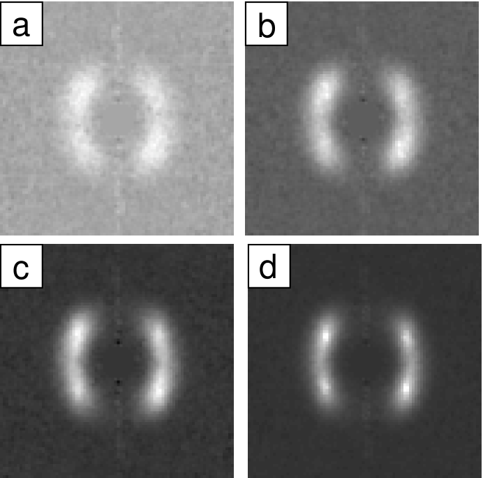
FIG. 1.: Time-averaged structure factors $S({\bf k})$ of the fluctuations for (a) $\epsilon=-0.46$, (b) $\epsilon=-0.21$, (c) $\epsilon=-0.11$, and (d) $\epsilon=-0.08$. The four peaks correspond to the zig and zag modes which are seen also in the extended-chaos state for large conductivity and $\epsilon>0$. The director is in the horizontal direction.

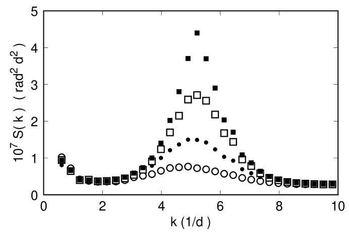
FIG. 2.: The structure factor $S(k)$ for $\epsilon$ = -0.08 (solid squares), -0.11 (open squares), -0.21 (solid circles), and -0.46 (open circles).

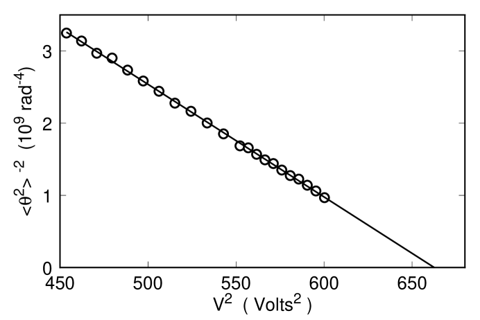
FIG. 3.: The inverse square of the mean-square director-angle fluctuations $<\theta^{2}>^{-2}$ as a function of the applied voltage-amplitude $V^{2}$. The intercept of the straight-line fit to the data with the horizontal axis gives $V_{c}^{2}$.

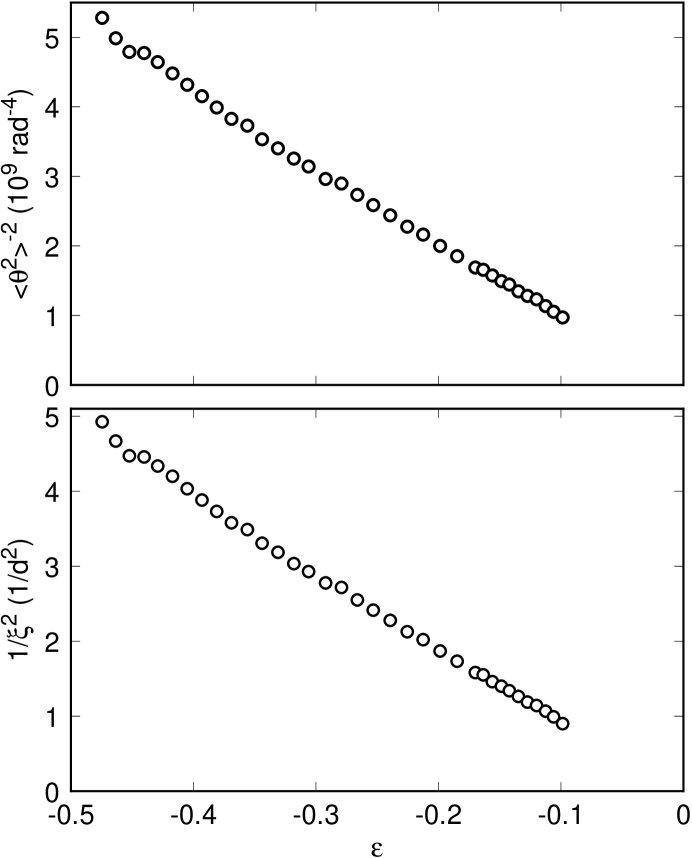
FIG. 4.: Top: The inverse square of the mean-square director-angle fluctuation $<\theta^{2}>^{-2}$ as a function of $\epsilon\equiv V^{2}/V_{c}^{2}-1$. Bottom: The inverse square $1/\xi^{2}$ of the average two-point correlation length derived from the width of S(k) in Fig. 2.

FIG. 5.: The inverse lifetime $1/\tau$ of the spatially uniform state vs. $\epsilon$. The solid line is based on a potential thermal-activation model.

REFERENCES

- [1] For a recent review, see for instance, M. C. Cross and P.C. Hohenberg, Rev. Mod. Phys. 65, 851 (1993).
- [2] E. Moses, F. Fineberg, and V. Steinberg, Phys Rev. A 35, 2757 (1987).
- [3] R. Heinrichs, G. Ahlers, and D. S. Cannell, Phys. Rev. A 35, 2761 (1987).
- [4] O. Thual and S. Fauve, J. Phys. (France) 49, 1829 (1988).
- [5] K. Lerman, E. Bodenschatz, D.S. Cannell, and G. Ahlers, Phys. Rev. Lett. 70, 3572 (1993).
- [6] Two-dimensional pulses were found[7] in numerical studies of CGL equations for a subcritical bifurcation and two modes.
- [7] R.J. Deissler and H.R. Brand, Phys. Rev. A 44, R3411 (1991).
- [8] M. Dennin, G. Ahlers, and D. S. Cannell, Science 272, 388 (1996).
- [9] M. Dennin, G. Ahlers, and D. S. Cannell, Phys. Rev. Lett. 77, 2475 (1996).
- [10] J.B. Swift and P.C. Hohenberg, Phys. Rev. A 15, 319 (1977).
- [11] Y. Tu, Phys. Rev. E 56, 3765R (1997).
- [12] H. Riecke and L. Kramer, private communication.
- [13] M. Treiber and L. Kramer, Mol. Cryst. Liq. Cryst. 261, 2164 (1995).
- [14] I. Rehberg, S. Rasenat, M. de la Torre-Juarez, W. Schöpf, F. Hörner, G. Ahlers and H.R. Brand, Phys. Rev. Lett. 67, 596 (1991).
- [15] See, for instance, H.A. Kramers, Physica 7, 284 (1940); and S. Chandrasekhar, Rev. Mod. Phys. 15, 1 (1943).
- [16] For a discussion of the properties of liquid crystals, see for instance P.G. de Gennes, The Physics of Liquid Crystals (Clarendon Press, Oxford, 1973).
- [17] For a discussion of early experiments, see for instance I. Rehberg, B.L. Winkler, M. de la Torre Juárez, S. Rasenat, and W. Schöpf, Festkörperprobleme 29, 35 (1989).
- [18] M. Dennin, D.S. Cannell, and G. Ahlers, Phys. Rev. E 57, in print (Jan. 1 1998).
- [19] S. Rasenat, G. Hartung, B.L. Winkler and I. Rehberg, Experiments in Fluids 7, 412 (1989).
- [20] Oblique-roll fluctuations below the bifurcation point were observed first by F.D. Hörner and I. Rehberg (unpublished) [see F.D. Hörner, Ph.D. Thesis, University of Bayreuth, Bayreuth, Germany, 1996 (unpublished)].
- [21] For isotropic systems, the effect of external noise is discussed by P.C. Hohenberg and J.B. Swift, Phys. Rev. A 46, 4773 (1992).
- [22] The exact value of depends on the algorithm used for detecting worms. We measured the variance of images as a function of time. When the variance had grown by a specified factor , we assumed that the first worm had formed. We used ; but the method showed surprisingly little dependence on .
- [23] It was important to wait long enough between successive measurements. When the voltage was switched off and then on again too soon, worms appeared quickly at the same places as in the previous run. Typically we had to wait 45 min to get statistically independent data. The reason for this “memory effect” is not clear. One possibility is that strong convective flow in the previous worm disordered the director field severely, introducing many defects which require much longer than a few director relaxation times (of order one second) to heal. Another possibility is that the nonlinear flowfield created a lateral variation of the impurity (iodine) concentration which had to diffuse away.