Spatio-temporal dynamics of coupled array of Murali-Lakshmanan-Chua circuits

Abstract

The circuit recently proposed by Murali, Lakshmanan and Chua (MLC) is one of the simplest non-autonomous nonlinear electronic circuits which shows a variety of dynamical phenomena including various bifurcations, chaos and so on. In this paper we study the spatio-temporal dynamics in one and two dimensional arrays of coupled MLC circuits both in the absence as well as in the presence of external periodic force. In the absence of any external force, the propagation phenomena of travelling wave front and its failure have been observed from numerical simulations. We have shown that the propagation of travelling wave front is due to the loss of stability of the steady states (stationary front) via subcritical bifurcation coupled with the presence of necessary basin of attraction of the steady states. We also study the effect of weak coupling on the propagation phenomenon in one dimensional array which results in the blocking of wave front due to the existence of a stationary front. Further we have observed the spontaneous formation of hexagonal patterns (with penta-hepta defects) due to Turing instability in the two dimensional array. We show that a transition from hexagonal to rhombic structures occur by the influence of external periodic force. We also show the transition from hexagons to rolls and hexagons to breathing (space time periodic oscillations) motion in the presence of external periodic force. We further analyse the spatio-temporal chaotic dynamics of the coupled MLC circuits (in one dimension) under the influence of external periodic forcing. Here we note that the dynamics is critically dependent on the system size. Above a threshold size, a suppression of spatio-temporal chaos occurs, leading to a space-time regular (periodic) pattern eventhough the single MLC circuit itself shows a chaotic behaviour. Below this critical size, however, a synchronization of spatiotemporal chaos is observed.

I Introduction

Coupled nonlinear oscillators in the form of arrays arise in many branches of science. These coupled arrays are often used to model very many spatially extended dynamical systems explaining reaction-diffusion processes. One can visualize such an array as an assembly of a number of subsystems coupled to their neighbours, or as coupled nonlinear networks (CNNs) [Chua & Yang, 1988; Chua, 1995]. Theoretically one can consider a system of coupled ordinary differential equations (odes) to represent a macroscopic system, in which each of the odes corresponds to the evolution of the individual subsystem. Specific examples are the coupled array of anharmonic oscillators [Marín & Aubry, 1996], Josephson junctions [Watanabe et al., 1995], continuously stirred tank reactors (CSTR) exhibiting travelling waves [Dolnik & Marek, 1988; Laplante & Erneux, 1992], propagation of nerve impulses (action potential) along the neuronal axon[Scott, 1975], the propagation of cardiac action potential in the cardiac tissues [Allesie et al., 1978] and so on. For the past few years several investigations have been carried out to understand the spatio-temporal behaviours of these coupled nonlinear oscillators and systems. The studies on these systems include the travelling wave phenomena, Turing patterns, spatio-temporal chaos and synchronization [Feingold et al., 1988; Muñuzuri et al., 1993; Pérez-Muñuzuri et al., 1993; Sobrino et al., 1993; Pérez-Muñuzuri et al., 1994, Pérez-Muñuzuri et al., 1995; Kocarev & Parlitz, 1996].

One of the interesting behaviours of these coupled oscillators is that they can exhibit a failure mechanism for travelling waves which cannot be observed in the homogeneous continuous models [Keener, 1987]. Similar failure phenomena in the nerve impulse propagation have been observed in biological experiments [Balke et al., 1988; Cole et al., 1988].

Recently various spatio-temporal patterns have been found in discrete realizations of the reaction-diffusion models by means of arrays of coupled nonlinear electronic circuits [Pérez-Muñzuri et al., 1993]. For example Pérez-Muñuzuri and coworkers studied the various spatio-temporal patterns in a model of discretely coupled Chua’s circuits. This system is a three variable model and coupled to its neighbours by means of a linear resistor. In this paper we consider similar arrays of coupled nonlinear electronic circuits consisting of Murali-Lakshmanan-Chua (MLC) circuits as a basic unit, which is basically a two variable model. The dynamics of the driven MLC circuit including bifurcations, chaos, controlling of chaos and synchronization has been studied by Murali et al. [1994a; 1994b; 1995; Lakshmanan & Murali, 1996]. Of particular interest among coupled arrays is the study of diffusively coupled driven systems as they represent diverse topics like Faraday instability [Lioubashevski et al., 1996], granular hydrodynamics [Umbanhawar et al., 1996; Kudrolli et al., 1997], self organized criticality [Bak & Chen, 1991] and so on. Identification of localized structures in these phenomena has been receiving considerable attention very recently [Fineberg, 1996]. Under these circumstances, study of models such as the one considered in this paper can throw much light on the underlying phenomenon in diffusively coupled driven systems.

In the following by considering one and two dimensional arrays of coupled MLC circuits, we have studied the various spatio-temporal patterns in the presence as well as in the absence of external force. We present a brief description on the one and two dimensional arrays of MLC circuits in Sec. II. Then, in Sec. III, in the absence of periodic external force, we study the propagation phenomenon of travelling wave front and its failure below a critical diffusive coupling coefficient. We show that the propagation phenomenon occurs due to a loss of stability of the steady states via subcritical bifurcation coupled with the presence of necessary basin of attraction of the steady states for appropriate diffusive coupling coefficient. We also study the effect of weak coupling on the propagation phenomenon which causes a blocking in the propagation due to the presence of a stationary front at the weakly coupled cell. In addition we also study the onset of Turing instability leading to the spontaneous formation of hexagonal patterns in the absence of any external force.

Further as mentioned earlier it is of great physical interest to study the dynamics of the coupled oscillators when individual oscillators are driven by external forces. In Sec. IV, we study the spatio-temporal patterns in the presence of periodic external force and investigate the effect of it on the propagation phenomenon and Turing patterns. Depending upon the choice of control parameters, a transition from hexagons to regular rhombic structures, hexagons to rolls and then to breathing oscillations from hexagons are observed. The presence of external force with sufficient strength removes the penta-hepta defect pair originally present in the spontaneously formed hexagonal patterns leading to the formation of regular rhombic structures. The inclusion of external periodic force can also induce a transition from hexagons to rolls provided there are domains of small roll structures in the absence of force. We further show that in the region of Hopf-Turing instability, the inclusion of external periodic force with sufficiently small amplitude induces a type of breathing oscillations though the system shows a regular hexagonal pattern in the absence of any external force.

Finally, we also study the spatio-temporal chaotic dynamics of the one dimensional array of MLC circuits in Sec. V when individual oscillators oscillate chaotically. In this case, the emergence of spatio-temporal patterns depends on the system size. For larger size, above a critical number of cells, we observe a controlled space-time regular pattern eventhough the single MLC circuit itself oscillates chaotically. However, synchronization occurs for a smaller system size, below the threshold limit. Finally, in Sec. VI we give our conclusions.

II Arrays of Murali-Lakshmanan-Chua circuits

As mentioned in the introduction the circuit proposed by Murali, Lakshmanan and Chua (MLC) is one of the simplest second order dissipative nonautonomous circuit having a single nonlinear element [Murali et al., 1994a]. Brief details of its dynamics are given in the Appendix A for convenience. Here we will consider one and two dimensional arrays of such MLC circuits, where the intercell couplings are effected by linear resistors.

II.1 One-dimensional array

Fig. 1(a) shows a schematic representation of an one dimensional chain of resistively coupled MLC circuits. Extending the analysis of single MLC circuit as given in the Appendix A, the dynamics

Figure 1: (a) Circuit realization of an one dimensional array of coupled MLC circuits. (b) Graph of the function $h(x)$ Vs. $x$ for the parametric choice $\{m_{0},m_{1},m_{2},\epsilon\}=$ $\{-1.02,-0.55,-0.55,0\}$ in Eq. (2). (c) Graph showing $h(x)$ Vs. $x$ for the parametric choice $\{m_{0},m_{1},m_{2},\epsilon\}=\{-2.25,1.5,$ $0.25,0\}$ in Eq. (2).

of the one dimensional chain can be easily shown to be governed by the following system of equations, in terms of the rescaled variables (see Appendix A),

$$\dot{x}_{i} = y_{i}-h(x_{i})+D(x_{i+1}+x_{i-1}-2x_{i}),$$ (1a)

$$\dot{y}_{i} = -\sigma y_{i}-\beta x_{i}+F\sin\omega t,\,\,\,\,\,i=1,2,\cdots,N,$$ (1b)

where $D$ is the diffusion coefficient, $N$ is the chain length and $h(x)$ is a three segment piecewise linear function representing the current voltage characteristic of the Chua’s diode,

$$h(x)=\left\{\begin{matrix}\epsilon+m_{2}x+(m_{0}-m_{1}),&x\geq x_{2}\cr\epsilon+m_{0}x,&x_{1}\leq x\leq x_{2}\cr\epsilon+m_{1}x-(m_{0}-m_{1}),&x\leq x_{1}.\end{matrix}\right.$$ (2)

In (2) $m_{0}$, $m_{1}$ and $m_{2}$ are the three slopes. Depending on the choice of $m_{0}$, $m_{1}$ and $m_{2}$ one can fix the characteristic curve of the Chua’s diode. Here $\epsilon$ corresponds to the dc offset. Of special importance for the present study are the two forms of $h(x)$ shown in Figs. 1(b) and 1(c). Fig. 1(b) corresponds to the choice of the parameters $\{m_{0},m_{1},m_{2},\epsilon\}=\{-1.02,-0.55,-0.55,0\}$ while Fig. 1(c) corresponds to the parameters $\{m_{0},m_{1},m_{2},\epsilon\}=\{-2.25,1.5,0.25,0\}$. As noted in the Appendix A, the significance of the characteristic curve in Fig. 1(b) is that it admits interesting bifurcations and chaos, while Fig. 1(c) corresponds to the possibility of bistable states with asymmetric nature which is a prerequisite for observing wave front propagation and its failure. In the following studies we will consider a chain of $N=100$ MLC circuits.

II.2 Two-dimensional array

As in the case of one dimensional array one can also consider a two dimensional array with each cell in the array being coupled to four of its nearest neighbours with linear resistors. The model equation can be now written in dimensionless form as

$$\dot{x}_{i,j}=y_{i,j}-h(x_{i,j})+D_{1}(x_{i+1,j}+x_{i-1,j}+x_{i,j+1}+x_{i,j-1}-4x_{i,j})\equiv f(x_{i,j},y_{i,j}),$$ (3a)

$$\dot{y}_{i,j}=-\sigma y_{i,j}-\beta x_{i,j}+D_{2}(y_{i+1,j}+y_{i-1,j}+y_{i,j+1}+y_{i,j-1}-4y_{i,j})+F\sin\omega t\equiv g(x_{i,j},y_{i,j}),\;\;\;i,j=1,2,\cdots,N.$$

This two dimensional array has $N\times N$ cells arranged in a square lattice. In our numerical study we will again take $N=100$.

In the following sections we present some of the interesting dynamical features of the array of MLC circuits such as propagation of wave front and its failure, effect of weak coupling in the propagation, Turing patterns, effect of external periodic forcing in the Turing patterns and spatio-temporal chaotic dynamics. We have used zero flux boundary conditions for the study of propagation phenomenon and Turing patterns and periodic boundary conditions for the study of spatio-temporal chaos.

III Spatio-temporal patterns in the absence of external force: Travelling wave phenomenon and Turing patterns

Transport processes in living tissues, chemical and physiological systems have been found to be associated with special types of waves called travelling waves. Earlier, continuous models were created to describe the wave propagation phenomenon in these systems, but these failed to cover all the important aspects of travelling wave behaviour. One of the most important of them is the so called travelling wave propagation failure, occurring at weak coupling between cells. It has been proved by Keener [1987] that propagation failure cannot be observed in a continuous, one variable, homogeneous reaction-diffusion system. Therefore to study this kind of phenomenon, one has to use discrete models. Recently travelling wave phenomenon and its failure have been studied in arrays of discretely coupled Chua’s circuits [Pérez-Muñuzuri et al., 1993]. Wave propagation and its failure have also been observed even in one variable models like discrete Nagumo equation [Leenaerts, 1997]. In this section we carry out a study of such wave propagation phenomenon in one and two dimensional arrays of Murali-Lakshmanan-Chua’s (MLC) circuit oscillators, without forcing, and investigate the mechanism by which such a failure occurs.

III.1 Propagation phenomenon and its failure in one-dimensional array

In order to observe wave front propagation in the one dimensional array of MLC circuits, we numerically integrated the Eqs. (1) using fourth order Runge-Kutta method. In this analysis we fix the parameters at $\{\beta,\sigma,m_{0},m_{1},m_{2},\epsilon,$ $F\}=\{1.0,1.0,-2.25,1.5,.25,0,0\}$ so that the system admits bistability and this choice leads to the asymmetry characteristic curve for the Chua’s diode as shown in Fig. 1(c). The existence of bistable state in the asymmetric case is necessary to observe a wave front. Zero flux boundary conditions were used in the numerical computations, which in this context mean setting $x_{0}=x_{1}$ and $x_{N+1}=x_{N}$ at each integration step; similar choice has been made for the variable $y$ also. To start with, we will study in this section the force-free case, $F=0$, and extend our studies to the forcing case $(F\neq 0)$ in the next section.

The choice of the values of the parameters guarantees the existence of two stable equilibrium points $P^{+}_{i}=\{\sigma(m_{1}-m_{0}-\epsilon)/(\beta+m_{2}\sigma)$, $\beta(m_{0}-m_{1}-\epsilon)/(\beta+m_{2}\sigma)\}$ and $P^{-}_{i}=\{\sigma(m_{1}-m_{0}-\epsilon)/(\beta+m_{1}\sigma)$, $\beta(m_{0}-m_{1}-\epsilon)/(\beta+m_{1}\sigma)\}$ for each cell. In the particular case, corresponding to the above parametric choice, each cell in the array has three equilibrium points at $P^{+}_{i}=(3.0,-3.0)$, $P^{-}_{i}=(-1.5,1.5)$ and $P^{0}_{i}=(0,0)$. Out of these three equilibrium points, $P^{+}_{i}$ and $P^{-}_{i}$ are stable while $P^{0}_{i}$ is unstable. Due to the asymmetry in the function $h(x)$ for the present parametric choices, the basin of attraction of the point $P^{+}_{i}$ is much larger than that of $P^{-}_{i}$ and it is harder to steer a trajectory back into the basin $P^{-}_{i}$ once it is in the basin of $P^{+}_{i}$.

Now we choose an initial condition such that the first few cells in the array are excited to the $P_{i}^{+}$ state (having a large basin of attraction compared to that of $P_{i}^{-}$) and the rest are set to $P_{i}^{-}$ state. In other words a wave front in the array is obtained by means of the two stable steady states. On actual numerical integration of Eqs.(1) with $N=100$ and with the diffusion coefficient

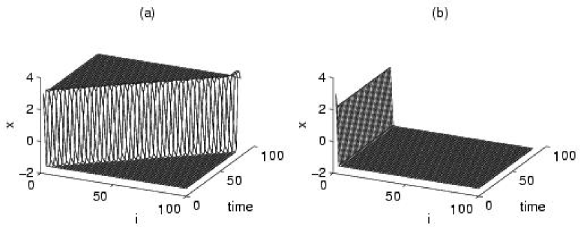
Figure 2: Space-time plot showing (a) propagation of wave fronts in one dimensional array (100 cells) of MLC circuits for $D=2.0$ and (b) propagation failure for $D=0.4$.

chosen at a higher value, $D=2.0$, a motion of the wave front towards right (see Fig. 2(a)) is observed, that is a travelling wave front is found. After about 80 time units the wave front reaches the $100^{\mbox{th}}$ cell so that all the cells are now settled at the more stable state $(P_{i}^{+})$ as demonstrated in Fig. 2(a). When the value of $D$ is decreased in steps and the analysis is repeated, the phenomenon of travelling wavefronts continues to be present.

However, below a critical value of the diffusion coefficient $(D=D_{c})$ a failure in the propagation has been observed, which in the present case turns out to be $D=D_{c}=0.4$. This means that the initiated wavefront is unable to move as time progresses and Fig. 2(b) shows the propagation failure for $D=0.4$.

III.2 Propagation failure mechanism: A case study of 5 coupled oscillators

To understand the failure mechanism, we have carried out a detailed case study of an array of five coupled MLC circuits, represented by the following set of equations. We have verified our conclusions for the case of 3, 4, 6 and 7 oscillators also. The analysis can be in principle extended to arbitrary but finite number of oscillators. From Eq. (1), the present array can be represented by the following set of ten coupled first order odes:

$$\dot{x}_{1} = y_{1}-h(x_{1})+D(x_{2}-x_{1}),$$

$$\dot{x}_{2} = y_{2}-h(x_{2})+D(x_{1}-2x_{2}+x_{3}),$$

$$\dot{x}_{3} = y_{2}-h(x_{3})+D(x_{2}-2x_{3}+x_{4}),$$

$$\dot{x}_{4} = y_{4}-h(x_{4})+D(x_{3}-2x_{4}+x_{5}),$$

$$\dot{x}_{5} = y_{5}-h(x_{5})+D(x_{4}-x_{5}),$$

$$\dot{y}_{j} = -\sigma y_{j}-\beta x_{j},\,\,\,\,\,\,j=1,2\ldots,5,$$ (4)

where $h(x)$ is as given in Eq. (2) and the parameters are fixed at $\beta=1$, $\sigma=1$, $m_{0}=-2.25$, $m_{1}=1.5$, $m_{2}=0.25$ and $\epsilon=0$.

III.2.1 Numerical analysis

By carrying out a numerical analysis of the system (III.2) with zero flux boundary conditions, we identify the following main results.

We solve the above system of equations (III.2) for the chosen initial condition $\{x_{1}(0),$ $x_{2}(0),$ $x_{3}(0),$ $x_{4}(0),$ $x_{5}(0)\}$ $=$ $\{3.0,$ $3.0,$ $-1.5,$ $-1.5,$ $-1.5\}$ and $y_{i}(0)=-x_{i}(0)$, $i=1,2\ldots 5,$ for different values of the diffusion coefficient $D$ in the region $D\in(0,1.0)$. Note that the values $x_{1}(0)=x_{2}(0)=3.0$ and $x_{3}(0)=x_{4}(0)=x_{5}(0)=-1.5$ correspond to the stable equilibrium points $P_{i}^{+}$ and $P_{i}^{-}$, respectively, of the uncoupled MLC oscillators. When $D$ is decreased downwards from $1.0$ we find that in the region $D>0.4$ propagation of wavefront occurs as in Fig. 2(a) (of the $N=100$ cells system). At the critical value $D=0.4$, the wavefront fails to propagate and asymptotically ends up in a stationary wavefront which is nearer to the initial condition (as in Fig. 2(b)). The wavefront failure phenomenon persists for all values of $0\leq D\leq 0.4$.

On the other hand, if we choose the initial condition as $\{x_{1}(0),$ $x_{2}(0),$ $x_{3}(0),$ $x_{4}(0),$ $x_{5}(0)\}$ $=$ $\{2.7990,$ $2.1709,$ $1.7803,$ $-1.4433,$ $-1.4923\}$ and $y_{i}(0)=-x_{i}(0)$, $i=1,2,..5,$ then the critical value $D$, where wavefront propagation failure occurs, turns out to be at a slightly higher value $D=D_{c}=0.4703$.

III.2.2 Linear stability analysis

In order to understand the failure mechanism of wavefront propagation we consider all the possible steady states (equilibrium states) associated with Eqs.(III.2) for nonzero values of $D$. It is easy to check that Eq. (III.2) possesses a maximum of $3^{5}=243$ steady states. First we consider the three trivial steady states which can be easily obtained by considering $x_{1}=x_{2}=x_{3}=x_{4}=x_{5}$ and $y_{1}=y_{2}=y_{3}=y_{4}=y_{5}$, namely, $X_{p}^{+}$ $=$ $(3.0,-3.0,3.0,-3.0,3.0,-3.0,3.0,-3.0,3.0,-3.0)$, $X_{p}^{0}$ $=$ $(0,0,0,0,0,0,0,0,0,0)$ and $X_{p}^{-}$ $=$ $(-1.5,1.5,-1.5,1.5,-1.5,1.5,-1.5,1.5,-1.5,1.5)$. (Here the suffix $p$ indicates that the steady states are the same as that of the $D=0$ case, namely $P_{i}^{+}$, $P_{i}^{0}$ and $P_{i}^{-}$). From a linear stability analysis (details are given in Appendix B) we can easily conclude that the steady states $X_{p}^{+}$ and $X_{p}^{-}$ are stable while $X_{p}^{0}$ is unstable irrespective of the value of the diffusion coefficient $D$. Then any initial condition in the neighbourhood of $X_{p}^{\pm}$ will evolve into $X_{p}^{\pm}$ asymptotically. Also one has to note that, due to asymmetry in the function $h(x)$, the basin of $X_{p}^{+}$ is much larger than that of $X_{p}^{-}$.

Since we are interested here to understand the propagation failure mechanism, we concentrate on those steady states which possess stationary wavefront structures near to the two types of chosen initial conditions in the numerical analysis discussed in Sec. III.2.1. Out of the 243 available steady states, we select a subset of them, $X_{s}=\{X_{s}^{+},X_{s}^{0},X_{s}^{-}\}$, which is nearer to the numerically chosen initial state. These three steady states are defined in Eqs.(13) of Appendix B. They are identified such that the components $x_{1s}$ and $x_{2s}$ are in the right extreme segment of the characteristic curve, Fig. 1(c), while $x_{4s}$ and $x_{5s}$ are in the left extreme segment. On the other hand $x_{3s}$ is allowed to be in any one of the three segments. The reason for such a choice is that we are looking for the formation of a wavefront which is closer to the chosen initial conditions in Sec. III.2.1. The corresponding forms of $h(x_{i})$ as given in Eq. (2) are then introduced in Eqs.(III.2) to find the allowed steady states. Then $X_{s}^{+}$ corresponds to the case in which $x_{3s}$ as well as $x_{1s}$ and $x_{2s}$ are in the right most segment while the rest are in the left most segment and $X_{s}^{0}$ and $X_{s}^{-}$ correspond to the cases in which $x_{3s}$ is, respectively, in the middle and the left extreme segments of the characteristic curve while $x_{1s}$, $x_{2s}$ and $x_{4s}$, $x_{5s}$ are chosen as in $X_{s}^{+}$. These steady states may be explicitly obtained as a function of the diffusion coefficient $D$, whose forms are given in Appendix B.

We now consider the linear stability of these steady states $X_{s}^{+}$, $X_{s}^{0}$ and $X_{s}^{-}$. The corresponding stability (Jacobian) matrices are obtained from the linearized version of Eq. (III.2), whose form is given in Eq. (16). The eigenvalues are evaluated by numerical diagonalization of (16) as a function $D$ and the stability property analysed. It has been found that out of these three steady states both $X_{s}^{+}$ and $X_{s}^{-}$ are stable for $D<0.4703$ in which all of the eigenvalues of (16) are having negative real parts, while $X_{s}^{0}$ is unstable for all values of $D>0$. However, the real part of atleast one of the eigenvalues associated with each of $X_{s}^{+}$ and $X_{s}^{-}$ changes its sign to positive value at $D=0.4703$ and thereby both the stationary fronts, $X_{s}^{+}$ as well as $X_{s}^{-}$, also lose their linear stability at this critical value. Thus for $D>0.4703$, all the three steady states $X_{s}^{+}$, $X_{s}^{0}$ and $X_{s}^{-}$ are linearly unstable.

First let us consider the second of the initial conditions chosen in Sec. III.2.1. At and above the critical value $D=0.4703$, all the three steady states are unstable and so the system transits to the other nearby steady states. These are also found to be unstable by a similar analysis, ultimately ending up in the only nearby available stable state which is $X_{p}^{+}$ $=$ $((3.0,-3.0),$ $(3.0,-3.0),$ $(3.0,-3.0),$ $(3.0,-3.0),$ $(3.0,-3.0))$, thereby explaining the propagation of the wavefront starting from the initial condition $X(0)$ $=$ $\{(2.7990,$ $-2.7990),$ $(2.1709,-2.1709),$ $(1.7803,-1.7803),$ $(-1.4433,1.4433),$ $(-1.4923,1.4923)\}$ (which is the second of the numerical results given in Sec. III.2.1). However for $D<0.4703$, since $X_{s}^{+}$ is stable and is also quite closer to the initial state, the system settles down in this state itself and no propagation occurs, thereby explaining the phenomenon of propagation failure as a subcritical bifurcation when the diffusion coefficient $D$ is increased from $0$ upwards. Note that eventhough $X_{s}^{-}$ is also stable, it is far away from the initial state and so no transition to this state will occur. A table of these steady states $X_{s}^{+}$ and $X_{s}^{-}$ as a function of $D$ (Table 2) is given confirming that $X_{s}^{+}$ is always nearer to the initial state compared to $X_{s}^{-}$.

Now let us consider the first of the initial conditions of our numerical analysis (see Sec. III.2.1), where wavefront propagation occurs at $D=0.4$ itself and not at $D=0.4703$, eventhough the steady states $X_{s}^{+}$ and $X_{s}^{-}$ are still linearly stable in the region $0.4\leq D<0.4703$. In order to understand this aspect, we start analysing the nature of the basin of attraction associated with the steady state $X_{s}^{-}$ for different $D$ values numerically (Note that for the present set of initial conditions $X_{s}^{-}$ is nearer to it than $X_{s}^{+}$). We find that the basin of $X_{s}^{-}$ shrinks as $D$ is increased from $0$ upwards and vanishes completely at $D=0.4703$. We also find that the chosen initial condition, $X(0)$ $=$ $((3.0,-3.0),$ $(3.0,-3.0),$ $(-1.5,1.5),$ $(-1.5,1.5),$ $(-1.5,1.5)$ falls fully within the basin of $X_{s}^{-}$ as long as $D<0.4$. However due to the

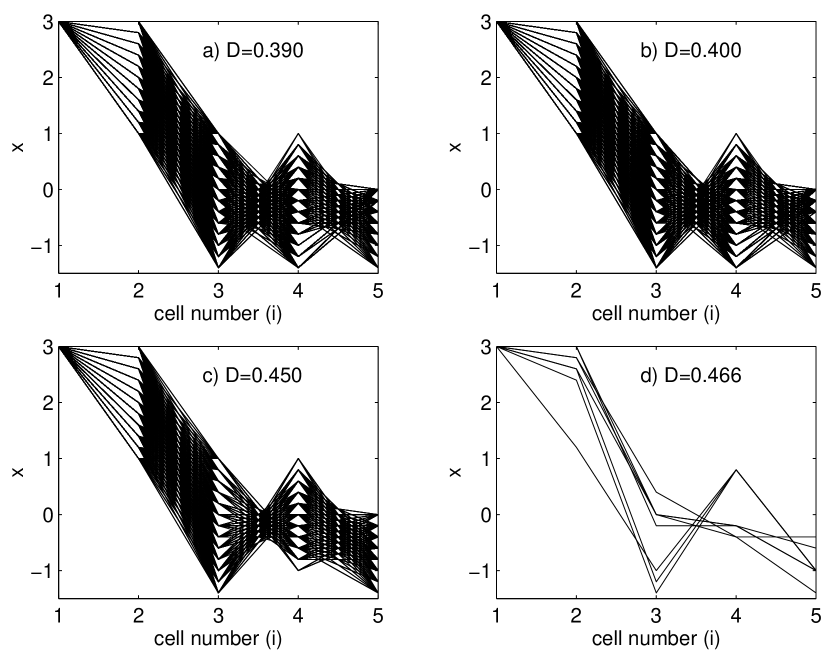
Figure 3: Figure showing partial basin for the steady state $X_{s}^{-}$ for various values of the diffusive coupling coefficient. In the figure each line corresponds to an initial condition. The figure is drawn by fixing the initial state of the first oscillator at $x_{1}(0)=3.0$, $y_{1}(0)=-3.0$ and for clarity decreasing the rest downwards in steps of 0.2.

shrinking nature of the basin as $D$ increases (as given in Figs. (3)), a part of the initial state falls outside the basin for $D>0.4$ (Figs. 3(b)-(d)). As a result the chosen initial condition does not end up in the stationary front $X_{s}^{-}$ for $0.4<D<0.4703$ indicating a global instability (eventhough the state is linearly stable). Therefore propagation starts to occur as soon as $D>0.4$, while it fails for $D\leq 0.4$ and it finally ends in the stable state $X_{p}^{+}$ described in the previous case. However, if an initial condition which happens to fall completely within the basin of attraction of $X_{s}^{\pm}$, the propagation starts to occur only for values of $D>0.4703$. In fact this is what happens for the second chosen initial condition ($X(0)$ $=$ $\{(2.7990,-2.7990),$ $(2.1709,-2.1709),$ $(1.7803,-1.7803),$ $(-1.4433,1.4433),$ $(-1.4923,1.4923)\}$, as explained above (Note that the basin structure shown in Fig. 3 does not cover this case).

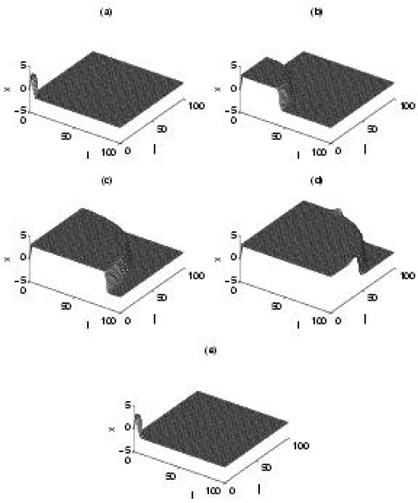
Figure 4: Three dimensional plot showing propagation of two dimensional wave fronts ($100\times 100)$ at various time units (a) $T=0$, (b) $T=50$, (c) $T=100$ and (d) $T=125$ for $D_{1}=2.0$ and $D_{2}=0$ and (e) the same plot for propagation failure case $D_{1}=0.4$ and $D_{2}=0$ at $T=1000\,\,t.u$.

In conclusion, the propagation failure of wave fronts in arrays of coupled nonlinear oscillators is essentially due to the existence of stationary fronts (stable steady states) near to the initial states for low diffusion coefficients, below a certain critical value, which lose stability via subcritical bifurcation. This coupled with the existence of necessary basin of attraction (for a global stability) of the steady state gives rise to the specific critical value of $D=D_{c}$ above which propagation begins for a given initial condition.

III.3 Propagation phenomenon in two-dimensional array

For studying the propagation phenomenon in two dimensional array of coupled MLC circuits, we have considered the case in which $F=0$, $D_{1}\neq 0$ and $D_{2}=0$. The propagation of wave front and its failure have been observed as in the case of one dimensional array. A two dimensional array of $100\times 100$ coupled MLC circuits has been considered for the numerical simulation with initial conditions chosen such that the first few cells in the array are excited to the $P^{+}_{i}$ state and the other cells are set at the $P^{-}_{i}$ state. Figs. 4(a)-4(d) show the propagation of the wave front in the two dimensional array for $D_{1}=2.0$ and $D_{2}=0$ at various time units. Again, below a certain critical diffusion coefficient, $D_{1}=0.4$, propagation failure occurs. One such case is illustrated in Fig. 4(e) for $D_{1}=0.4$ and $D_{2}=0$. The phenomenon can again be explained through a linear stability analysis as in the case of the one dimensional array.

III.4 Effect of weak coupling

In the above, the investigation has been made by considering the system as an ideal one (as far as the circuit parameters are concerned). But from a practical point of view, there are defects in the coupling parameters which may result in a weak coupling at any of the cell in the array. In the following we study the effect of such weak coupling on the propagation of wave front.

Let us consider a weak coupling at the $k^{\mbox{th}}$ cell. By this we mean that the $k^{\mbox{th}}$ cell in the array is coupled to its nearest neighbour $(k+1)^{\mbox{th}}$ and $(k-1)^{\mbox{th}}$ cells by resistors with slightly higher values than that of the others. We have studied the effect of this defect on the propagation of wave fronts. Numerical simulations have been carried out by considering an one dimensional array with 100 cells, where the initial conditions are chosen as in the case of propagation phenomenon in regular one dimensional arrays (see Sec. III.1). From the numerical simulation results, we find that there is an abrupt stop in the propagation when the wave front reaches the weakly coupled cell. This happens when the coupling coefficient on either side of the $k^{\mbox{th}}$ cell in the array has a value even above the critical value $(D=0.4)$ for propagation failure discussed in Sec. III.1.

Figure 5: Figure showing the effect of weak coupling at the 25${}^{\mbox{th}}$ cell in the one dimensional array (Eq. (3)). (a) three dimensional space-time plot and (b) density plot.

Fig. 5 shows a blocking in the propagation of the wave front when the coupling coefficients on either side of the $k^{\mbox{th}}$ cell $(k=25)$, which we call as $D_{k}$, is set to $0.47173$ with the rest of the coupling coefficients set to $1$ $(D=1)$. We observe that the actual blocking occurs when the wave front reaches the $k^{\mbox{th}}$ cell. We can say this is a kind of failure in the propagation (because the wavefront will never reach the last cell (that is the $100^{\mbox{th}}$ cell in the array) by means of blocking.

As far as the initial conditions are concerned, since the system is in the propagation region $(D=1.0)$ any choice of initial condition of wavefront structure will lead to uniform propagation upto the weakly coupled cell. Now our motivation is to find the property of the above uniform wavefront when it reaches the weakly coupled cell.

One can analyse the above phenomenon by means of a linear stability analysis of the steady states as in the case of propagation phenomenon in Sec. III.2. We consider again as an example the system of five coupled MLC circuits as in Eqs.(III.2) in which the middle cell ($x_{3}$) is now taken as an example to be coupled weakly to its neighbours, respectively $x_{2}$ and $x_{4}$. This set up can be represented by the following set of ten coupled odes:

$$\dot{x}_{1} = y_{1}-h(x_{1})+D(x_{2}-x_{1}),$$

$$\dot{x}_{2} = y_{2}-h(x_{2})+D(x_{1}-x_{2})+D_{k}(x_{3}-x_{2}),$$

$$\dot{x}_{3} = y_{2}-h(x_{3})+D_{k}(x_{2}-2x_{3}+x_{4}),$$

$$\dot{x}_{4} = y_{4}-h(x_{4})+D_{k}(x_{3}-x_{4})+D(x_{5}-x_{4}),$$

$$\dot{x}_{5} = y_{5}-h(x_{5})+D(x_{4}-x_{5}),$$

$$\dot{y}_{j} = -\sigma y_{j}-\beta x_{j},\,\,\,\,\,\,j=1,2\ldots,5,$$ (5)

Here $D_{k}$ corresponds to the coupling coefficient of the weakly coupled cell and other parameters are the same as in (III.2). As in Sec. III.2, we calculated the steady states associated with (III.4) and analysed the linear stability properties.

Let us now consider the three steady states of the system (III.4), namely, $X_{s}=\{X_{s}^{+},X_{s}^{0},X_{s}^{-}\}$ which possess wavefront structures near the chosen initial conditions. These steady states can be found as discussed in Sec. III.2. By fixing $D=1.0$, we analyse the stability of $X_{s}$ as a function of $D_{k}$. We find that, the steady states, $X_{s}^{\pm}$ are linearly stable for values of $D_{k}$, $0\leq D_{k}\leq 0.4717$ and become unstable for $D_{k}>0.4717$ via subcritical bifurcation. However $X_{s}^{0}$ state continues to be unstable irrespective of the value of $D_{k}$.

At this point, one may think of an array with large number of MLC circuits. Since all the cells, except the $k^{\mbox{th}}$ cell, have diffusion coefficient $D=1.0$ which is in the propagation region, the appropriately chosen initial condition will evolve as a propagating front upto the weakly coupled cell. When this wave front reaches the weakly coupled cell, the existence of the stationary front $X_{s}^{-}$ for the array due to the presence of the weakly coupled cell will block the propagating front and hence it will end up in the stationary front $X_{s}^{-}$ asymptotically for $D_{k}\leq 0.4717$. For $D_{k}>0.4717$, the stationary state $X_{s}^{-}$ is no longer stable and hence the propagation occurs without any blocking. Thus the blocking of the wave front can also be attributed to the existence of a stable stationary front when weak coupling is present in the system.

III.5 Turing patterns

Another interesting dynamical phenomenon in the coupled arrays is the formation of Turing patterns. These patterns are observed in many reaction diffusion systems when a homogeneous steady state which is stable due to small spatial perturbations in the absence of diffusion becomes unstable in the presence of diffusion[Turing, 1952]. To be specific, the Turing patterns can be observed in a two variable reaction-diffusion system when one of the variables diffuses faster than the other and undergo Turing bifurcation, that is, diffusion driven instability[Turing, 1952; Murray, 1989].

Treating the coupled array of MLC circuits as a discrete version of a reaction-diffusion system, one can as well observe the Turing patterns in this model also. For this purpose, one has to study the linear stability of system (3) near the steady state. In continuous systems, the linear stability analysis is necessary to arrive at the conditions for diffusion driven instability. A detailed derivation of the general conditions for the diffusion driven instability can be found in Murray[1989]. For discrete cases one can follow the same derivation as in the case of continuous systems by considering solutions of the form $\exp i(kj-\lambda t)$ [Murray 1989; Muñuzuri et al., 1995]. Here $k$ and $\lambda$ are considered to be independent of the position $j$ $(j=1,2,\cdots,N)$. For Eq. (3), the criteria for the diffusion driven instability can be derived by finding the conditions for which the steady states in the absence of diffusive coupling are linearly stable and become unstable when the coupling is present. One can easily derive from a straightforward calculation that the following conditions should be satisfied for the general reaction-diffusion system of the form given by Eq. (3):

$$f_{x}+g_{y} < 0,$$

$$f_{x}g_{y}-f_{y}g_{x} > 0,$$

$$f_{x}D_{2}-g_{y}D_{1} > 0,$$

$$(f_{x}D_{2}-g_{y}D_{1})^{2}-4D_{1}D_{2}(f_{x}D_{2}-g_{y}D_{1}) > 0.$$ (6)

The critical wave number for the discrete system (3) can be obtained as

$$\cos(k_{c})=1-\displaystyle{f_{x}D_{2}-g_{y}D_{1}\over 4D_{1}D_{2}}.$$ (7)

Combining Eqs. (III.5)-(7), one obtains[Muñuzuri et al., 1995] the condition for the Turing instability such that

$${f_{x}D_{2}-g_{y}D_{1}\over 8D_{1}D_{2}}\leq 1.$$ (8)

We apply these conditions to the coupled oscillator system of the present study. For this purpose, we fix the parameters for the two-dimensional model (3) as $\{\beta,\sigma,\epsilon,m_{0},m_{1},m_{2}\}=\{0.8,$ $0.92,0.1,-0.5,0.5,0.5\}$ and verify that this choice satisfies the conditions (III.5) to (8). The numerical simulations are carried out using an array of size $100\times 100$ and random initial conditions near the steady states are chosen

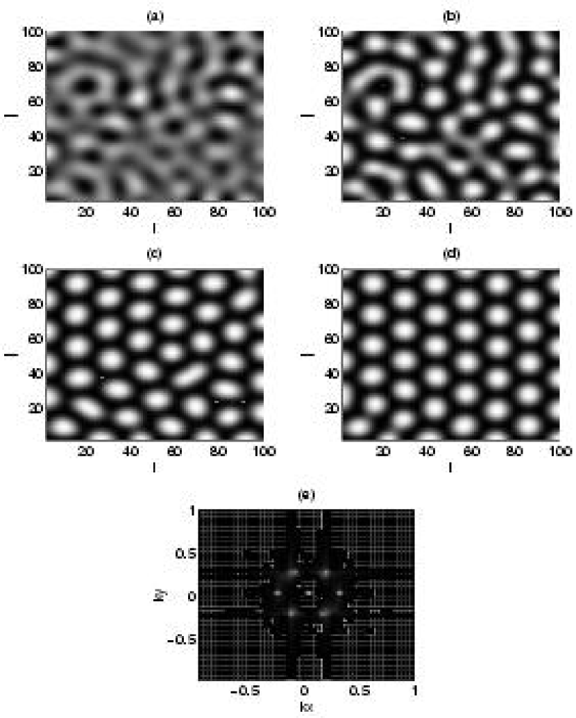
Figure 6: The spontaneous formation of Turing patterns in an array of $100\times 100$ oscillators for the parameters $\beta=0.8$, $\sigma=1$, $m_{0}=-0.5$, $m_{1}=0.5$, $m_{2}=0.5$, $\epsilon=0.1$, $F=0.0$, $\omega=0.75$, $D_{1}=1$ and $D_{2}=10$ in Eq. (3) at various time units (a) $T=50$, (b) $T=100$, (c) $T=500$ and (d) $T=2000$ (e) the same figure (d) in the Fourier space.

for the $x$ and $y$ variables. Figs. 6(a)-6(d) show how the diffusion driven instability leads to stable hexagonal pattern (Fig. 6(d)) after passing through intermediate stages (Figs. 6(a)-6(c)). Fig. 6(e) shows the two dimensional Fourier spectrum of the hexagonal pattern (Fig. 6(d)). Further, the spontaneously formed patterns are fairly uniform hexagonal patterns having a penta-hepta defect pair. These defects are inherent and very stable. We note that such Turing patterns have already been observed in an array of coupled Chua’s circuits[Muñuzuri et al, 1995]. However, our aim here is to investigate the effect of external forcing on these patterns, which is taken up in the next section.

IV Spatio-temporal patterns in the presence of periodic external force

The effect of external fields on a variety of dynamical systems has been studied for a long time as driven systems are very common from a practical point of view. For example, in a large number of dynamical systems including the Duffing oscillator, van der Pol oscillator and the presently studied MLC circuits, temporal forcing leads to a variety of complex dynamical phenomena such as bifurcations, quasiperiodicity, intermittency, chaos and so on[Guckenheimer & Holmes, 1983; Hao Bai-Lin, 1984; Lakshmanan & Murali,1996]. Also the studies on the effect of external fields in spatially extended systems have been receiving considerably increasing interest in recent times [Pismen, 1987; Walgraef, 1988; 1996]. Particularly, with the recent advances in identifying localized and oscillating structures and other spatio-temporal patterns in driven nonlinear dissipative systems such as granular media, driven Ginzburg-Landau equations and so on, it is of considerable interest to study the effects of forcing on array of coupled systems such as (3). Motivated by the above, we investigate the effect of external forcing in the propagation of wave front and formation of Turing patterns in the coupled MLC circuits in one and two dimensions.

IV.1 Effect of external forcing on the propagation of wave fronts

In this subsection we study the effect of external forcing on the propagation of wave fronts. For this purpose we consider an one dimensional array of coupled MLC circuits with initial and boundary conditions as discussed in Sec. III.1. Now we perform the numerical integration by the inclusion of external periodic force of frequency $\omega=0.75$ in each cell of the array (see Eq. (1)). By varying the strength, $F$, of the external force we study the behaviour of the propagating wave front in comparison with the force free case ($F=0$) as discussed in Sec. III.1. We find that in the propagation region ($D>D_{c}$), the effect of forcing is just to introduce temporal oscillations and the propagation continues without

Figure 7: Propagation phenomena in the presence of forcing: (a) Propagation of wavefront for $D=2.0$ and $F=0.6$ and (b) The partial propagation observed for the $D=0.22$ and $F=0.6$.

any disturbance (see Fig. 7(a)) as in the case $F=0$ (Fig. 2(a)). Of course this can be expected as the external force is periodic in time. However, interesting things happen in the propagation failure region discussed in Sec. III.1. In this region, beyond a certain critical strength of the external forcing, the wavefront tries to move a little distance and then stops, leading to a partial propagation. Fig. 7(b) shows such a partial propagation observed for $F=0.6$ and $D=0.22$ (This may be compared with Fig. 2(b)). The phenomenon can be explained by considering the propagation failure mechanism discussed in Sec. III.2 in which one may look for a spatially stationary and temporally oscillating wavefront. The initial wavefront tries to settle in the nearby stationary state. However, the system will take a little time and space to settle due the effect of forcing combined with the transient behaviour of the system. Thus the inclusion of external forcing in the propagation failure region can induce the wavefront to achieve a partial propagation.

IV.2 Transition from hexagons to rhombs

It is well known that the defects are inherent in very many natural pattern forming systems. In most of the pattern forming systems, the observed patterns are not ideal. For example, the patterns are not of perfect rolls or hexagons or rhombs. A commonly observed defect in such systems is the so called penta-hepta defect (PHD) pair which is the bound state of two dislocations [Tsimring, 1996]. Experiments on spatially extended systems often show the occurrence of PHD in spontaneously developed hexagonal patterns[Pantaloni & Cerisier, 1983]. In the present case also, the existence of PHD pair can be clearly seen from Fig. 6(d). In such a situation, it is important to study the effect of external periodic force in the coupled arrays of MLC circuits.

Now we include a periodic force with frequency $\omega$ and amplitude $F$ in each cell of the array and we numerically integrate Eqs.(3) using fourth order Runge-Kutta method with zero flux at boundaries. By fixing the frequency of the the external periodic force as $\omega=0.75$ and varying the amplitude ($F$) we analyse the pattern which emerges spontaneously. Interestingly for $F=0.25$, the defects (PHD pair) which are present in the absence of external force (Fig. 6(d)), gets removed resulting in the

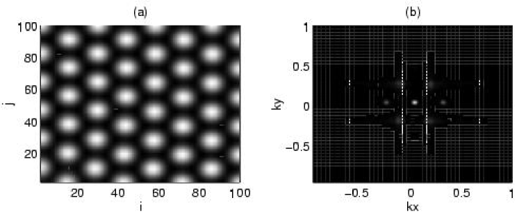
Figure 8: Figure showing the formation of rhombic structures in the presence of forcing. (a) Gray scale plot of the rhombic pattern for $F=0.25$ and (b) The same figure in Fourier space.

transition to a regular rhombic array. Fig. 8(a) shows the gray scale plot of the pattern observed for $F=0.25$ and the corresponding plot in Fourier domain (Fig. 8(b)). Thus, from the above we infer that the inclusion of external periodic force can cause a transition from hexagonal pattern to rhombic structures. We note that Pérez-Muñuzuri et al. have observed, in arrays of coupled Chua’s circuits, similar transition from hexagons to rhombs by means of sidewall forcing [Pérez-Muñuzuri et al., 1995]. However in our case we apply forcing simultaneously to all the cells, in order to mimic situations such as application in vertically vibrated granular media[Umbanhowar et al., 1996].

IV.3 Transition from hexagons to rolls

In addition to the transition from hexagons to rhombs by the influence of external periodic force, there are also other possible effects due to it. To realize them, we consider a different set of parametric

Figure 9: Figure showing the transition from hexagons to rolls for $\{\beta,$ $\sigma,$ $\epsilon,$ $m_{0}$, $m_{1},$ $m_{2}\}$ $=$ $\{0.734722,$ $0.734722,$ $0.15,$ $-0.874,$ $-0.4715,$ $-0.4715\}$ with $D_{1}=1$ and $D_{2}=5$. (a) $F=0$, (b) $F=0.15$, (c) $F=0.35$ and (d) $F=0.45$.

choice $\{\beta,\sigma,m_{0},m_{1},m_{2}\}$ $=$ $\{0.734722,$ $0.734722,$ $-0.874,$ $-0.4715,$ $-0.4715\}$ with $\epsilon=0.15$, $D_{1}=1.0$ and $D_{2}=5.0$. For this choice the system shows hexagonal patterns with defects including domains of small roll structures (Fig. 9(a)).

Now when the external periodic force is included a transition in the pattern from hexagonal structure to rolls starts appearing. By fixing the frequency of the external periodic force again at $\omega=0.75$, we observed the actual transition from hexagons to rolls as we increase the forcing amplitude ($F$). Figs. 9(b)-9(d) show the gray scale plots for $F=0.15$, $0.35$ and $0.45$, respectively. Obviously the transition is due to the existence of small roll structures in the pattern for $F=0$ which nucleates the formation of rolls in the presence of forcing.

IV.4 Breathing oscillations

In the above, we have shown that the inclusion of the external periodic force can make a transition from one stationary pattern to another stationary pattern like the transition from hexagons to rolls. Besides these, are there any time varying patterns? As mentioned above, patterns such as localized and breathing oscillations have considerable

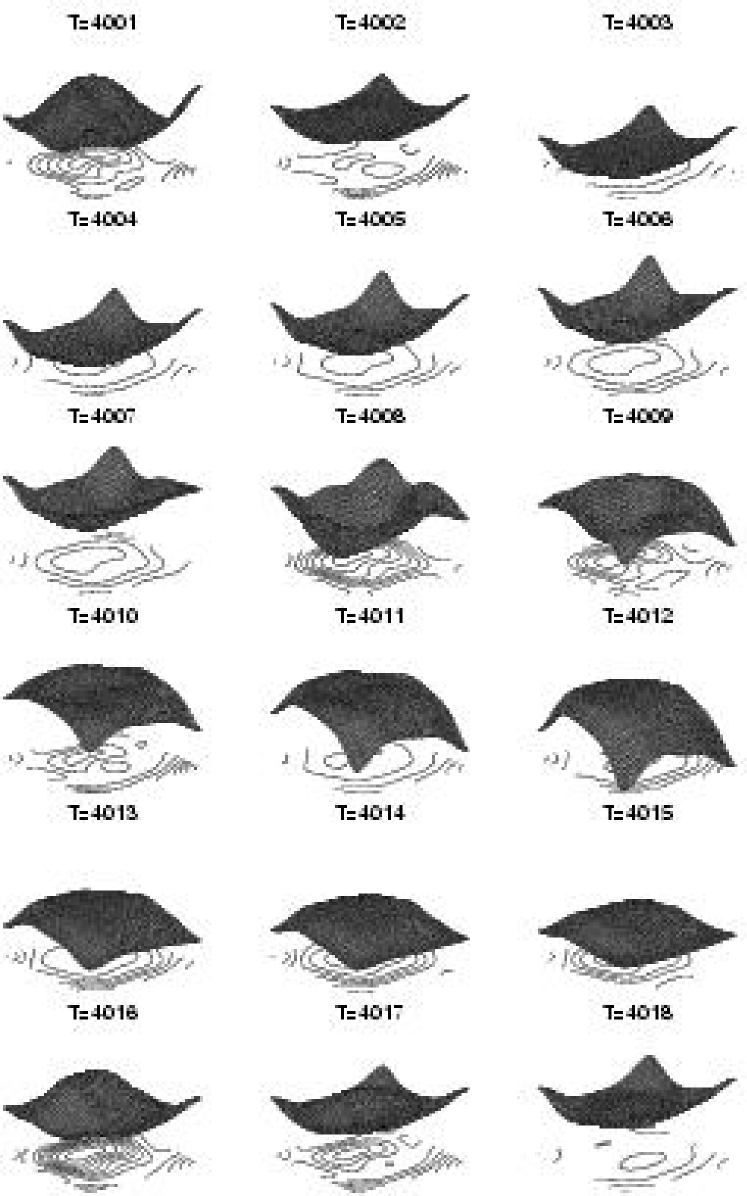
Figure 10: Snapshots showing the breathing oscillations for $F=0.05$ and $\{\beta,$ $\sigma,$ $\epsilon,$ $m_{0}$, $m_{1},$ $m_{2}\}$ $=$ $\{0.734722,$ $0.734722,$ $0.15,$ $-0.874,$ $-0.4715,$ $-0.4715\}$ with $D_{1}=2$ and $D_{2}=5$ for various time units starting from $T=4001$.

physical interest. In this regard, we considered the parameters $\{\beta,\sigma,\epsilon,m_{0},m_{1},m_{2}\}$ $=$ $\{0.734722,$ $0.734722,$ $0.10,$ $-0.874,$ $-0.4715,$ $-0.4715\}$ with $D_{1}=2.0$ and $D_{2}=5.0$ such that a regular hexagonal pattern is observed in the absence of external periodic force. From numerical simulations, we observed that a space-time periodic oscillatory pattern (breathing motion) sets in for a range of low values of $F$. Fig. 10 shows the typical snapshots of the oscillating pattern at various instants for the specific choice $F=0.05$. We have integrated over 10000 time units and the figure corresponds to the region $T=4000-4018$. Typically we find that the breathing pattern repeats itself approximately after a period $T=15.0$ in the range of our integration. One may conclude that the emergence of such breathing oscillations is due to the competition between the Turing and Hopf modes in the presence of external periodic force.

V Spatio-temporal chaos

Next we move on to a study of the spatio-temporal chaotic dynamics of the array of coupled MLC circuits when individual cells are driven by external periodic force. The motivation is that over a large domain of ($F$, $\omega$) values the individual MLC circuits typically exhibits various bifurcations and transition to chaotic motion (see Appendix A). So one would like to know how the coupled array behaves collectively in such a situation, for fixed values of the parameters. For this purpose, we set the parameters at $\{\beta,\sigma,\epsilon,m_{0},m_{1},$ $m_{2},\omega\}=\{1.0,1.015,0,-1.02,-0.55,-0.55,0.75\}$. In our numerical simulations, we have mainly considered the one dimensional array specified by Eq. (1) and assumed periodic boundary conditions. The choice of periodic boundary conditions here makes the calculation of Lyapunov exponents easier so as to understand the spatio-temporal chaotic dynamics of (1) in a better way.

V.1 Spatio-temporal regular and chaotic motion

Numerical simulations were performed by considering random initial conditions using fourth order Runge-Kutta method for seven choices of $F$ values. The coupling coefficient in Eq. (1) was chosen as $D=1.0$. Out of these, the first three lead to period-$T$, period-$2T$, period-$4T$ oscillations, respectively and the remaining choices

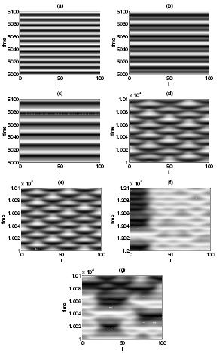
Figure 11: Spatio-temporal periodic oscillations in a grid of $100$ oscillators for the external periodic forcing strength (a) $F=0.05$, (b) $F=0.08$, (c) $F=0.09$, (d) $F=0.12$, (e) $F=0.13$, (f) $F=0.14$ and (g) $F=0.15$

correspond to chaotic dynamics of the single MLC circuit. Figs. 11(a)-11(g) show the space-time plots for $F=0.05$, $F=0.08$, $F=0.09$, $F=0.12$, $F=0.13$, $F=0.14$ and $F=0.15$, respectively. From the Figs. 11(a)-11(c), it can be observed that for $F=0.05$, $0.08$ and $0.09$ the MLC array also exhibits regular periodic behaviour with periods $T$, $2T$ and $4T$ respectively in time alone as in the case of the single MLC circuit. However, for $F=0.12$ and $0.13$(Figs. 11(d) and 11(e)) one obtains space-time periodic oscillations eventhough each of the individual uncoupled MLC circuits for the same parameters exhibits chaotic dynamics. We may say that a kind of controlling of chaos occurs due to the coupling, though the coupling strength is large here. From the above analysis it can be seen that the macroscopic system shows regular behaviour in spite of the fact that the microscopic subsystems oscillate chaotically. Finally for $F=0.15$ the coupled system shows spatio-temporal chaotic dynamics (Fig. 11(g)) and this was confirmed by calculating the Lyapunov exponents using the algorithm given by Wolf et al. [Wolf et al., 1985]. For example, we calculated the Lyapunov exponents for $N=50$ coupled oscillators (For $N=100$, it takes enormous computer time relatively which we could not afford at present) and we find the highest three exponents have the values $\lambda_{\mbox{max}}=\lambda_{0}=0.1001$, $\lambda_{1}=0.0776$, $\lambda_{2}=0.0092$ and the rest are negative (see next subsection for further analysis). We also note that for $F=0.14$, the system is in a transitional state as seen in Fig. 11(f).

V.2 Size dependence of the ST Chaos

Since the above study of spatio-temporal chaos involves a large number of coupled chaotic oscillators it is of great interest to analyse the size dependence of the dynamics of these systems. To start with, we consider the case of 10 coupled oscillators with periodic boundary conditions and numerically solve the system using fourth order Runge-Kutta method with the other parameters chosen as in Sec. V.1. The value of $F$ is chosen in the range $(0.12,0.15)$. We find that this set up shows different behaviour as compared to the 100 cell case. Actually the system gets synchronized to a chaotic orbit rather than showing periodic behaviour as in the case of 100 cells described above.

First we analyse the dynamics for $F=0.12$ by slowly increasing the system size from $N=10$. We noted that for the system size, $N\leq 42$ it gets synchronized to a chaotic orbit as mentioned above. We have also calculated the corresponding Lyapunov spectrum and found that there is one positive maximal Lyapunov exponent as long as $N\leq 42$. For example, for $N=42$, $\lambda_{\mbox{max}}=0.1162$, with the rest

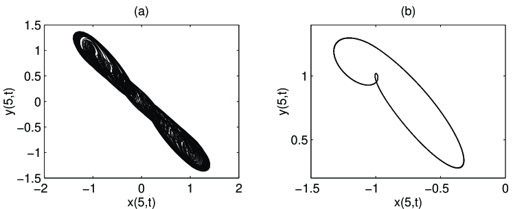
Figure 12: (a) The chaotic attractor at the $5^{\mbox{th}}$ cell for the synchronized state $(N=42)$ and (b) the periodic orbit in the $5^{\mbox{th}}$ cell for the controlled state $(N=43)$

of the exponents being negative. Fig. 12(a) shows the dynamics of the $5^{\mbox{th}}$ cell in the array and 13(a) depicts the space-time plot of the synchronized spatio-temporal chaos. The system shows entirely different behaviour when we increase the system size to $N=43$. As noted in the previous subsection, V.1, there occurs kind of suppression of spatio-temporal chaos. Fig. 12(b) shows the resultant periodic orbit in the $5^{\mbox{th}}$ cell of the array and Fig. 13(b) shows the space-time plot of the spatio-temporal periodic behaviour of the array. The maximal Lyapunov exponent is found to be negative in this case $(\lambda_{\mbox{max}}=-0.001474)$. We observed the same phenomenon for $F=0.13$ also.

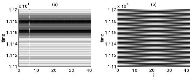
Figure 13: Space-time plot showing the size dependence of the dynamics in the coupled chaotic oscillators. (a) $N=42$ and (b) $N=43$.

Next we consider the case of $F=0.15$ in which the coupled system in the previous subsection showed spatio-temporal chaos. From numerical simulations, we again observed a synchronized motion for $N\leq 31$ and the corresponding Lyapunov spectrum shows one positive exponent only with all other exponents being negative. But for $N>31$, the coupled system shows spatio-temporal chaos. The Lyapunov spectrum in this case (for $N>31$) possesses multiple positive exponents. For example, for $N=43$, $(\lambda_{\mbox{max}}=\lambda_{0}=0.0997$, $\lambda_{1}=0.0633$, $\lambda_{2}=0.0038)$.

From the above analysis we see definite evidence that the spatio-temporal chaotic dynamics in coupled MLC circuits depends very much on the size of the system. A similar analysis can be performed to investigate the nature of the spatio-temporal dynamics on the strength of the coupling coefficient $D$. Preliminary analysis shows similar phenomenon at critical values of $D$. Further work is in progress on these lines.

VI Conclusions

In this paper we have discussed various spatiotemporal behaviours of the coupled array of Murali-Lakshmanan-Chua circuits in one and two dimensions. In the first part we have reported the propagation phenomenon of the travelling wave fronts and failure mechanism in the absence of external forcing. We have shown that the propagation phenomenon is due to the loss of stability of the steady states via subcritical bifurcation coupled with the presence of necessary basin of attraction of the steady states. The effect of weak coupling on the travelling wave phenomenon has also been studied. In the two dimensional array we studied the onset of Turing instability leading to the spontaneous formation of hexagonal patterns.

Introduction of external periodic force has been shown to lead to a partial propagation in the failure region of one dimensional array, while in the two dimensional array a transition from hexagons to rhombs take place. We have also showed that a transition from hexagons to rolls can occur by the influence of external periodic force provided domains of small roll structures already present in the absence of external force. Space-time breathing oscillations as a result of the competition between Hopf and Turing modes in the presence of external periodic force have also been observed. We have also studied the spatio-temporal chaotic dynamics and showed that the MLC array exhibits both periodic and chaotic dynamics as in the case of single oscillator. In the chaotic regime the dynamics is also critically dependent on the system size. For a large array, the collective behaviour shows periodic oscillations both in space and time eventhough the individual subsystems oscillate chaotically as the coupling brings the macroscopic system into a regular motion. On the other hand, below a critical size of the system, it gets synchronized to a chaotic orbit. The study of array of diffusively coupled driven nonlinear oscillators is of intrinsic interest as they represent many natural phenomena such as Faraday instability, patterns in granular media and so on. Of particular interest will be to look for localized structures in these systems. Whether such excitations exists in the present arrays of oscillators is a question to be answered in the near future. Work is in progress along these lines.

Appendix A Dynamics of the MLC circuit

The Murali-Lakshmanan-Chua circuit, Fig. 14(a), is the simplest second order dissipative nonautonomous circuit, consisting of Chua’s diode as the only nonlinear element[Murali et al., 1994a]. This circuit contains a capacitor $(C)$, an inductor $(L)$, a linear

Figure 14: A single MLC circuit

resistor $(R)$, an external periodic forcing $(f\sin\Omega t)$ and a Chua’s diode. By applying the Kirchoff’s laws to this circuit, the governing equations for the voltage $v$ across the capacitor $C$ and the current $i_{L}$ through the inductor $L$ are represented by the following set of two first order nonautonomous differential equations:

$$C\frac{dv}{dt} = i_{L}-g(v),$$

$$L\frac{di_{L}}{dt} = -Ri_{L}-R_{s}i_{L}-v+f\sin\Omega t,$$ (9)

where $g(v)$ is a piecewise linear function corresponding to the characteristic of the Chua’s diode $(N)$ and is given by

$$g(v_{R})=\left\{\begin{matrix}\epsilon^{\prime}+G_{2}v_{R}+(G_{0}-G_{1}),&v_{R}\geq B_{p}\cr\epsilon^{\prime}+G_{0}v_{R},&-B_{p}\leq v_{R}\leq B_{p}\cr\epsilon^{\prime}+G_{1}v_{R}-(G_{0}-G_{1}),&v_{R}\leq-B_{p}\end{matrix}\right.$$ (10)

The piecewise nature of the characteristic curve of Chua’s diode is obvious from Eq. (10)[Murali et al., 1994a]. The slopes of left, middle and right segments of the characteristic curve are $G_{1}$, $G_{0}$ and $G_{2}$, respectively. $-B_{p}$ and $B_{p}$ are the break points and $\epsilon^{\prime}$ corresponds to the dc offset in the Chua’s diode. Rescaling Eq. (A) as $v=xB_{p}$, $i_{L}=GyB_{p}$, $G=1/R$, $\omega=\Omega C/G$ $t=\tau C/G$ and $\epsilon=\epsilon^{\prime}/G$ and then redefining $\tau$ as $t$ the following set of normalized equations are obtained:

$$\dot{x} = y-h(x),$$

$$\dot{y} = -\beta x-\sigma y+F\sin\omega t,$$ (11)

with

$$h(x)=\left\{\begin{matrix}\epsilon+m_{2}x+(m_{0}-m_{1}),&x\geq x_{2}\cr\epsilon+m_{0}x,&x_{1}\leq x\leq x_{2}\cr\epsilon+m_{1}x-(m_{0}-m_{1}),&x\leq x_{1}\end{matrix}\right.,$$ (12)

where $\beta=(C/LG^{2})$, $\sigma=(C/LG^{2})(1+GR_{s})$ and $F=(f\beta/B_{p})$. Obviously $h(x)$ takes the form as in Eq. (2) with $m_{0}=G_{0}/G$, $m_{1}=G_{1}/G$ and $m_{2}=G_{2}/G$. The dynamics of Eq. (A) depends on the parameters $\beta$, $\sigma$, $m_{0}$, $m_{1}$, $m_{2}$, $\epsilon$, $\omega$ and $F$.

The rescaled parameters corresponding to the experimental observations reported in Murali et al.[1994a] correspond to $\beta=1.0$, $\sigma=1.015$, $m_{0}=-1.02$, $m_{1}=-0.55$, $m_{2}-0.55$, $\epsilon=0$ and $\omega=0.75$. By varying $F$ one can observe the familiar period doubling bifurcations leading to chaos and several periodic windows in

Figure 15: Bifurcation diagram in the $F$-$x$ plane of the MLC circuit for the parametric choice (a) $\{\beta,\sigma,m_{0},m_{1},m_{2},\epsilon,\omega\}$ $=\{1.0,1.015,-1.02,-0.55,-0.55,0,0.75\}$ and (b) $\{\beta,\sigma,m_{0},$ $m_{1},m_{2},\epsilon,\omega\}=\{1.0,1.0,-2.25,$ $1.5,0.25,0,0.75\}$.

the MLC circuit. Fig. 15(a) shows the one parameter bifurcation diagram in the $F$-$x$ plane [$F\in(0,0.7)$]. A summary of the bifurcations that occur in this case for different $F$ values is given in Table 1. Further it is of great interest to consider the parametric choice $\{m_{0},m_{1},m_{2},\epsilon,\beta,\sigma,\omega\}=\{-2.25,1.5,0.25,0.0,$ $1.0,1.0,0.75\}$ which corresponds to the function $h(x)$ having the form as shown in Fig. 1(c). This choice of parameters provides the possibility of bistability nature in the asymmetric case in the absence of periodic forcing. In this case one can easily observe from numerical simulations that the MLC circuit admits only limit cycles for $F\in(0,0.7)$. The bifurcation diagram in the $F$-$x$ plane is depicted in Fig. 15(b).

Table 1: Summary of bifurcation phenomena of Eq.(A3)

amplitude $(F)$	description of attractor
$0<F\leq 0.071$	period-1 limit cycle
$0.071<F\leq 0.089$	period-2 limit cycle
$0.089<F\leq 0.093$	period-4 limit cycle
$0.093<F\leq 0.19$	chaos
$0.19<F\leq 0.3425$	period-3 window
$0.3425<F\leq 0.499$	chaos
$0.499<F\leq 0.625$	period-3 window
$0.625<F$	period-1 boundary

In the main text, we also consider other choices of the parameters depending on the phenomenon we are interested in. The corresponding values are given at the appropriate places in the text.

Appendix B Steady states and Jacobian matrix of the system of 5 coupled oscillators (Eqs. (III.2))

The steady states of Eq. (III.2) can be obtained explicitly as a function of the diffusion coupling coefficient $D$ by introducing the appropriate form of $h(x_{i})$ from Eq. (2). Out of the $3^{5}=243$ possible steady states we consider here a subset $X_{s}=\{X_{s}^{+},X_{s}^{0},X_{s}^{-}\}$ and $X_{p}=\{X_{p}^{+},X_{p}^{0},X_{p}^{-}\}$ discussed in Sec. III.2.2.

To obtain the set $X_{s}$ we proceed as follows. The components $x_{1s}$ and $x_{2s}$ are in the right extreme segment of the characteristic curve, Fig. 1(c), while $x_{4s}$ and $x_{5s}$ are in the left extreme segment. Therefore choosing $h(x_{i})$ $=$ $m_{2}x+(m_{0}-m_{1})$ for $i=1,2$ and $h(x_{i})$ $=$ $m_{1}x-(m_{0}-m_{1})$ for $i=4,5$ (see Eq. (2)), we obtain

$$X^{+}_{s}=\{x_{1s}^{+},y_{1s}^{+},x_{2s}^{+},y_{2s}^{+},x_{3s}^{+},y_{3s}^{+},x_{4s}^{+},y_{4s}^{+},x_{5s}^{+},y_{5s}^{+}\}$$ (13a)

for $$h(x_{3})=m_{2}x+(m_{0}-m_{1})$$,

$$X^{0}_{s}=\{x_{1s}^{0},y_{1s}^{0},x_{2s}^{0},y_{2s}^{0},x_{3s}^{0},y_{3s}^{0},x_{4s}^{0},y_{4s}^{0},x_{5s}^{0},y_{5s}^{0}\}$$ (13b)

for $$h(x_{3})=m_{0}x$$ and

$$X^{-}_{s}=\{x_{1s}^{-},y_{1s}^{-},x_{2s}^{-},y_{2s}^{-},x_{3s}^{-},y_{3s}^{-},x_{4s}^{-},y_{4s}^{-},x_{5s}^{-},y_{5s}^{-}\}$$ (13c)

for $h(x_{3})=m_{1}x-(m_{0}-m_{1})$. Explicitly solving Eqs. (III.2) we can write

$$x_{1s}^{+} = \frac{3}{K}(16D^{3}+620D^{2}+550D+125),$$

$$x_{2s}^{+} = \frac{3}{K}(16D^{3}+500D^{2}+550D+125),$$

$$x_{3s}^{+} = \frac{3}{K}(16D^{3}+260D^{2}+400D+125),$$

$$x_{4s}^{+} = \frac{1.5}{K}(32D^{3}-200D^{2}-400D-125),$$

$$x_{5s}^{+} = \frac{1.5}{K}(32D^{3}-560D^{2}-550D-125),$$

$$y_{i}^{+} = -x_{i}^{+},\,\,\,\,\,\,i=1,2,\ldots 5,$$

$$x_{1s}^{-} = -\frac{3}{L}(32D^{4}-920D^{3}-3200D^{2}-2750D-625),$$

$$x_{2s}^{-} = -\frac{3}{L}(32D^{4}-560D^{3}-2000D^{2}-2000D-625),$$

$$x_{3s}^{-} = -\frac{1.5}{L}(64D^{4}+320D^{3}+1700D^{2}+2000D+625),$$

$$x_{4s}^{-} = -\frac{1.5}{L}(64D^{4}+1280D^{3}+3500D^{2}+2750D+625),$$

$$x_{5s}^{-} = -\frac{1.5}{L}(64D^{4}+1760D^{3}+3800D^{2}+2750D+625),$$

$$y_{i}^{-} = -x_{i}^{-},\;\;\;\;\;\;i=1,2,\ldots 5,$$

$$x_{1s}^{0} = \frac{15}{M}(64D^{3}+44D^{2}-50D-25),$$

$$x_{2s}^{0} = \frac{15}{M}(48D^{3}+44D^{2}-30D-25),$$

$$x_{3s}^{0} = \frac{30D}{M}(8D^{2}+12D+5),$$

$$x_{4s}^{0} = -\frac{7.5}{M}(32D^{3}-32D^{2}-40D-25),$$

$$x_{5s}^{0} = -\frac{7.5}{M}(64D^{3}+32D^{2}-50D-25),$$

$$y_{i}^{0} = -x_{i}^{0},\,\,\,\,\,\,i=1,2,\ldots 5.$$ (15)

with

$$K=112D^{3}+620D^{2}+550D+125.$$

$$L=256D^{4}+1880D^{3}+3800D^{2}+2750D+625.$$

and

$$M=64D^{4}+320D^{3}+140D^{2}-250D-125.$$

The stability determining eigenvalues are the roots of the characteristic equations of the Jacobian matrix for the linearised version of Eq. (III.2):

$$J(X_{s})=\begin{pmatrix}-h_{x_{1}}-D&D&0&0&0&1&0&0&0&0\cr D&-h_{x_{2}}-2D&D&0&0&0&1&0&0&0\cr 0&D&-h_{x_{3}}-2D&D&0&0&0&1&0&0\cr 0&0&D&-h_{x_{4}}-2D&D&0&0&0&1&0\cr 0&0&0&D&-h_{x_{5}}-D&0&0&0&0&1\cr-1&0&0&0&0&-1&0&0&0&0\cr 0&-1&0&0&0&0&-1&0&0&0\cr 0&0&-1&0&0&0&0&-1&0&0\cr 0&0&0&-1&0&0&0&0&-1&0\cr 0&0&0&0&-1&0&0&0&0&-1\end{pmatrix}.$$ (16)

where $h_{x}$ is the derivative of $h(x)$ with respect to $x$ evaluated at the steady states.

Particularly we can show that for the trivial steady states $X_{p}^{+}=(3.0$, $-3.0$, $3.0$, $-3.0$, $3.0$, $-3.0$, $3.0$, $-3.0$, $3.0$, $-3.0)$, and $X_{p}^{-}=(-1.5$, $1.5$,$-1.5$, $1.5$, $-1.5$, $1.5$, $-1.5$, $1.5$, $-1.5$, $1.5)$ are stable and $X_{p}^{0}=(0$, $0$, $0$, $0$, $0$, $0$, $0$, $0$, $0$, $0)$ is unstable. For example considering $X_{P}^{+}$, the Jacobian (16) takes the form

$$J(X_{P}^{+})=\begin{pmatrix}-1.5-D&D&0&0&0&1&0&0&0&0\cr D&-1.5-2D&D&0&0&0&1&0&0&0\cr 0&D&-1.5-2D&D&0&0&0&1&0&0\cr 0&0&D&-1.5-2D&D&0&0&0&1&0\cr 0&0&0&D&-1.5-D&0&0&0&0&1\cr-1&0&0&0&0&-1&0&0&0&0\cr 0&-1&0&0&0&0&-1&0&0&0\cr 0&0&-1&0&0&0&0&-1&0&0\cr 0&0&0&-1&0&0&0&0&-1&0\cr 0&0&0&0&-1&0&0&0&0&-1\end{pmatrix}.$$ (17)

Table 2: Stable steady states $X_{s}^{+}$ and $X_{s}^{-}$ for $0\leq D\leq 0.4703$. Only $x_{is},i=1,2\ldots 5$ are given. The values of $y$’s are obtained from the relation $y_{is}=-x_{is}$ (One may note that the second initial conditions $\{x_{1}(0),$ $x_{2}(0),$ $x_{3}(0),$ $x_{4}(0),$ $x_{5}(0)\}$ $=$ $\{2.7990,$ $2.1709,$ $1.7803,$ $-1.4433,$ $-1.4923\}$ and $y_{i}(0)=-x_{i}(0)$, $i=1,2,..5,$ chosen in Sec. III.2.1III.2.1 is closer to $X_{s}^{+}$ than $X_{s}^{-}$. Similarly the first of the initial conditions $\{x_{1}(0),$ $x_{2}(0),$ $x_{3}(0),$ $x_{4}(0),$ $x_{5}(0)\}$ $=$ $\{3.0,$ $3.0,$ $-1.5,$ $-1.5,$ $-1.5\}$ and $y_{i}(0)=-x_{i}(0)$, $i=1,2\ldots 5,$ is nearer to $X_{s}^{-}$ than $X_{s}^{+}$.)

	$D$	$x_{1s}$	$x_{2s}$	$x_{3s}$	$x_{4s}$	$x_{5s}$		$D$	$x_{1s}$	$x_{2s}$	$x_{3s}$	$x_{4s}$	$x_{5s}$
$X_{s}^{+}$	0.0000	3.0000	3.0000	3.0000	-1.5000	-1.5000	$X_{s}^{-}$	0.0000	3.0000	3.0000	-1.5000	-1.5000	-1.5000
	0.0100	3.0000	2.9997	2.9647	-1.4823	-1.4999		0.0100	2.9997	2.9647	-1.4823	-1.4999	-1.5000
	0.0200	3.0000	2.9989	2.9308	-1.4651	-1.4997		0.0200	2.9989	2.9308	-1.4651	-1.4997	-1.5000
	0.0300	2.9999	2.9977	2.8981	-1.4485	-1.4994		0.0300	2.9976	2.8981	-1.4485	-1.4994	-1.5000
	0.0400	2.9999	2.9960	2.8666	-1.4323	-1.4989		0.0400	2.9959	2.8666	-1.4323	-1.4989	-1.5000
	0.0500	2.9998	2.9939	2.8362	-1.4166	-1.4984		0.0500	2.9937	2.8362	-1.4166	-1.4984	-1.5000
	…	…	…	…	…	…		…	…	…	…	…	…
	0.4100	2.9571	2.8262	2.1655	-1.0393	-1.4351		0.4100	2.7921	2.1584	-1.0411	-1.4423	-1.4919
	0.4200	2.9550	2.8209	2.1537	-1.0321	-1.4327		0.4200	2.7853	2.1462	-1.0340	-1.4403	-1.4914
	0.4300	2.9528	2.8156	2.1422	-1.0250	-1.4303		0.4300	2.7784	2.1342	-1.0270	-1.4383	-1.4909
	0.4400	2.9506	2.8102	2.1308	-1.0180	-1.4279		0.4400	2.7715	2.1223	-1.0202	-1.4363	-1.4905
	0.4500	2.9484	2.8049	2.1196	-1.0111	-1.4254		0.4500	2.7646	2.1107	-1.0134	-1.4343	-1.4900
	0.4600	2.9461	2.7996	2.1087	-1.0043	-1.4230		0.4600	2.7577	2.0993	-1.0068	-1.4322	-1.4895
	0.4700	2.9435	2.7934	2.0937	-1.0162	-1.4234		0.4700	2.7508	2.0880	-1.0002	-1.4302	-1.4890

The eigenvalues of the above matrix (17) as a function of $D$ can be obtained by solving the corresponding characteristic equation. We have verified by numerical evaluation that all the eigenvalues of (17) have negative real parts for $D\geq 0$. Similarly all the eigenvalues corresponding to the steady state $X_{p}^{-}$ have negative real parts irrespective of the values of $D$ $(D\geq 0)$. We have also verified that atleast one of the eigenvalues corresponding to the state $X_{p}^{0}$ has positive real part for $D\geq 0$. Thus $X_{p}^{\pm}$ are stable, while $X_{p}^{0}$ is unstable for all values of $D\geq 0$.

Similarly one can obtain the stability properties of the set of steady states $X_{s}=\{X_{s}^{+},X_{s}^{0},X_{s}^{-}\}$, by substituting the appropriate expressions from (B) into (16). Numerical diagonalization of (16) for these steady states show that $X_{s}^{0}$ is unstable for all values of $D$, while $X_{s}^{+}$ and $X_{s}^{-}$ are stable for $0\leq D\leq 0.4703$ and unstable for $D>0.4703$ for the chosen initial conditions. The numerical values of $X_{s}^{\pm}$ in the stable region are given in Table 2 as a function of $D$.

x

References

- (1) Allesie, M. A., Bonke, F. I. M. & Scopman, T. Y. G. [1973] “Circus movement in rabit atrial muscle as a mechanism in tachycardia,” Circ. Res. 33, 54-62.
- (2) Bak, P., & Chen, K. [1991] “Self-organized criticality” Sci. Am. 264, 46.
- (3) Balke, C. W., Lesh, M. D., Spear, J. F., Kadish, A., Levine, J. H. & Moore, E. N. [1988] “Effects of cellular uncoupling on conduction in anisotropic canine ventricular myocardium,” Circ. Res. 63, 879-892.
- (4) Chua, L. O. and Yang, L. [1988] “Cellular neural networks: Theory,” IEEE Trans. Circ. Syst. 35, 1257-1272.
- (5) Chua, L. O. (Ed.) [1995] Special issue on “Nonlinear waves, patterns and spatio-temporal chaos in dynamic arrays,” IEEE Trans. Circ. Syst. 42, 557-823.
- (6) Cole, W. C., Picolne, J. B. & Sperelakis, N. [1988] “Gap junction uncoupling and discontinuous propagation in the heart,” Biophys. J. 53, 809-818.
- (7) Dolnik, M. & Marek, M. [1988] “Extincion of oscillations in forced and coupled reaction cells,” J. Phys. Chem. 92, 2452-2455.
- (8) Feingold, M., González, D. L., Piro, O. & Viturro, H. [1988] “Phase locking, period doubling and chaotic phenomena in externally driven excitable systems,” Phys. Rev. A 37, 4060-4063.
- (9) Fineberg, J [1996] “Physics of jumping sandbox,” Nature 382, 763-764
- (10) Guckenheimer, J. and Holmes, P. [1983] Nonlinear Oscillations, Dynamical Systems and Bifurcation of Vector fields (Springer Verlag, New York)
- (11) Hao Bai-Lin [1984] Chaos (World Scientific, Singapore)
- (12) Keener, J. P. [1987] “Propagation and its failure in coupled systems of excitable cells” SIAM J. Appl. Math 47, 556
- (13) Kocarev, L. & Parlitz, U. [1996] “Synchronizing spatiotemporal chaos in coupled nonlinear oscillators,” Phys. Rev. Lett. 77, 2206-2209.
- (14) Kudrolli, A., Wolpert, M & Gollub, J.P., [1997] “Cluster formation due to collisions in granular material,” Phys. Rev. Lett. 78, 1383-1386.
- (15) Lakshmanan, M. & Murali, K. [1995] “Experimental chaos from non-autonomous electronic circuits,” Phil. Trans. R. Soc. Lond. A 353, 33-46.
- (16) Lakshmanan, M. & Murali, K. [1996] Chaos in Nonlinear Oscillators: Controlling and Synchronization (World Scientific, Singapore).
- (17) Laplante, J. P. & Erneux, T. [1992] “Propagation failure and multiple steady states in an array of diffusion coupled flow reactors,” Physica A 188, 89-98.
- (18) Leenaerts, D. M . W. [1997] “Wave propagation and its failure in piecewise linear Nagumo equation” Proc. ECCTD’97.
- (19) Lioubasheski, O., Arbell, H. & Fineberg, J. [1996] “Dissipative solitary states in driven surface waves,” Phys. Rev. Lett. 76, 3959-3962.
- (20) Marín, J. L. & Aubry, S. [1996] “Breathers in nonlinear lattices: numerical calculation from the anticontinuous limit,” Nonlinearity 9, 1501-1528
- (21) Muñuzuri, A. P., Pérez-Muñuzuri, V., Pérez-Villar, V. & Chua, L. O. [1993] “Spiral wave in 2D array of nonlinear circuits,” IEEE Transactions Circuits and Systems 40, 872-877.
- (22) Muñuzuri, A. P., Pérez-Muñuzuri, V., Gómez-Gesteria, M., Chua, L. O. & Pérez-Villar, V. [1995] “Spatiotemporal structures in discretely-coupled arrays of nonlinear circuits: A Review,” Int. J. Bifurcation and Chaos 5, 17-50.
- (23) Murali, K., Lakshmanan, M. & Chua, L. O. [1994a] “The simplest dissipative non-autonomous chaotic circuit,” IEEE Trans. Circ. Sys. I41, 462-463
- (24) Murali, K., Lakshmanan, M. & Chua, L. O. [1994b] “Bifurcation and Chaos it the simplest dissipative non-autonomous chaotic circuit,” Int. J. Bifurcation and Chaos 4, 1511-1524
- (25) Murali, K., Lakshmanan, M. & Chua, L. O. [1995] “Controlling and synchronization of chaos in the simplest dissipative nonautonomous circuit” Int. J. Bifurcation and Chaos 5, 6498-6510
- (26) Murray, J. D. [1989] Mathematical Biology (Springer-Verlag, NewYork)
- (27) Pantaloni, J. & Cerisier, P. [1983] “Structure defects in Bénaed-Marangoni convection,” Cellular Structures and Instabilities, Leccture Notes in Physics 210, eds. Wesfreid. J. E. & Zaleski, S. (Springer-Verlag, Berlin)
- (28) Pérez-Muñuzuri, V., Gómez-Gesteria, M., Pérez-Villar, V. & Chua, L. O. [1993] “Travelling wave propagation in one dimensional fluctuating medium,” Int. J. Bifurcation and Chaos 3, 211-215.
- (29) Pérez-Muñuzuri, V., Alonso, M., Chua, L. O. & Pérez-Villar, V. [1994] “Resonance patterns in 1D arrays of coupled nonlinear excitable systems,” Int. J. Bifurcation and Chaos 4, 1631-1638.
- (30) Pérez-Muñuzuri V., Gómez-Gesteria, M., Muñuzuri, A. P., Chua, L. O. & Pérez-Villar [1995] “Sidewall forcing of hexagonal Turing patterns: Rhombic patterns,” Physica D 82, 195-204
- (31) Perraud, J. J., De Wit, A., Dulos, E., De Kepper, P., Dewel, G. & Borkmans, P. [1993] “One-dimensional spirals: a novel asynchronous chemical wave source”, Phys. Rev. Lett. 71, 1272-1275
- (32) Pismen, L. [1987] “Bifurcations of quasi-periodic and nonstationary pattern under external forcing”, Phys. Rev. Lett. 59, 2740
- (33) Scott, A. C. [1975] “The electrophysics of nerve fiber,” Rev. Mod. Phys. 47, 487-533.
- (34) Sobrino, T., Alonso, M., Pérez-Muñuzuri, V. & Pérez-Villar, V. [1993] “Reaction-diffusion process in a one-dimensional array of active nonlinear circuits,” Eur. J. Phys. 14, 74-79.
- (35) Tsimring, L. S. [1996] “Dynamics of penta-hepta defects in hexagonal patterns”, Physica D89, 368-380.
- (36) Turing, A. M. [1952] “The chemical basis of morphogenesis,” Phil. Trans. Roy. Soc. London B237, 37-72.
- (37) Umbanhowar, P. B., Melo, F. & Swinney, H. L. [1996] “Localized excitations in a vertically vibrated granular layers” Nature (London) 382, 793-796
- (38) Walgraef, D. [1988] “External forcing of spatio-temporal pattern” Europhys. Lett. 7, 485
- (39) Walgraef, D. [1996] Spatio-temporal Pattern Formation (Springer, New York) pp. 127-167
- (40) Watanabe, S., Strogatz, S. H., van der Zant, H. S. J. & Orlando, T. P. [1995] “Whirling modes and parametric instablilities in the discrete sine-Gordon equation: experimental tests in Josephson rings,” Phys. Rev. Lett. 74, 379-382.
- (41) Wolf, A., Swift, J. B, Swinney, H. L., and Vastano, J. A. [1985] “Determining Lyapunov exponents from a time series” Physica 16D 285-317.