Nature of Roll to Spiral-Defect-Chaos Transition

Abstract

We investigate the nature of the parallel-roll to spiral-defect-chaos (SDC) transition in Rayleigh-Bénard convection, based on the generalized Swift-Hohenberg model. We carry out extensive, systematic numerical studies by, on one branch, increasing the control parameter gradually from the parallel roll regime to the SDC regime and, on the other branch, decreasing it in the opposite manner. We find that the data of several time-averaged global quantities all form hysteretic loops from the two branches. We also discuss several possible scenarios for the transition and analyze our data for SDC accordingly. We conclude that the roll-to-SDC transition is first-order in character and that the correlation length diverges at the conduction to convection onset. We further postulate that this transition can be understood somewhat similar to the hexagon-to-roll transition in non-Boussinesq fluids. Finally we comment on the differences between our conclusion and those in two experiments.

I Introduction

Many nonequilibrium systems exhibit self-organized pattern-forming phenomena [2]. In the past few years, a new type of intrinsic pattern has emerged in many disciplines of science. These patterns are characterized by their extensive, irregular behavior in both space and time, which are known as spatiotemporal chaos (STC) [2]. STC typically exists in large size systems and its complexity increases dramatically with the system size [3]. Owing to its generic dynamical complexity, STC hence poses a great challenge to both experimentalists and theoreticians.

From the very beginning, Rayleigh-Bénard convection (RBC) has been a paradigm in the study of pattern formation in driven dissipative systems, because of its relative simplicity and high precision in controlled experiments [4]. RBC can occur when a thin horizontal layer of fluid is heated from below. The system is described by three dimensionless parameters [2]: (a) the Rayleigh number $R\equiv g\alpha d^{3}\Delta T/\kappa\nu$, in which $g$ is the gravitational acceleration, $d$ the layer thickness, $\Delta T$ the temperature gradient across the layer, $\alpha$ the thermal expansion coefficient, $\kappa$ the thermal diffusivity and $\nu$ the kinematic viscosity; (b) the Prandtl number $\sigma\equiv\nu/\kappa$; and, (c) the aspect ratio $\Gamma\equiv L/2d$ where $L$ is the horizontal size of the system. The Rayleigh number $R$ is the control parameter of the system; the Prandtl number $\sigma$ specifies the fluid properties. It is convenient to introduce a reduced control parameter $\epsilon\equiv(R-R_{c})/R_{c}$, where $R_{c}$ is the critical value of $R$ at which the fluid bifurcates from a static conductive state to a convective state.

RBC has been studied extensively in the literature [2, 4]. Theoretical analyses by Busse and his coauthors [5] predict that parallel roll states are stable inside a stability domain in $(R,k,\sigma)$ space with $k$ the wavenumber, which is known as the “Busse balloon”. Surprisingly, recent experiments [6, 7] and numerical studies [8, 9, 10], using systems with $\sigma\sim O(1)$ and large $\Gamma$, revealed that the parallel roll state yields to a spatiotemporally chaotic state even for states inside the Busse balloon. This spatiotemporally chaotic state, called spiral-defect-chaos (SDC), exhibits very complicated dynamics, illustrated by the interplay of numerous rotating spirals, patches of moving rolls, intricate grain boundaries, dislocations and other defects [6, 7]. Its discovery has since stimulated many experimental [6, 7, 11, 12, 13], theoretical [14, 15] and numerical [8, 9, 10, 16] efforts to understand it.

The nature of the parallel roll to SDC transition is one of the important questions with respect to SDC and has been investigated in several experimental and numerical studies [12, 13, 16]. By solving the generalized Swift-Hohenberg (GSH) model of RBC [17, 18, 19] for non-Boussinesq fluids with random initial conditions, two of us [16] characterized the transition by the behavior of time-averaged global quantities such as convective current $J$, vorticity current $\Omega$ (called vortex energy in Ref. [16]) and spectra entropy $\Xi$ [20]. It was found that the convective current seems to be smooth across the transition temperature $\epsilon_{T}$ but both the vorticity current and the spectra entropy seem to obey power-law behavior near $\epsilon_{T}$. However this study was unable to distinguish between a gradual or sharp transition. Despite its inconclusiveness on the nature of the roll-to-SDC transition, this study suggests that studying such time-averaged global quantities is quite useful. It hence motivated us to develop a phenomenological theory for STC, including SDC, in RBC [15]. In the theory, we made a random phase approximation for the spatiotemporally chaotic states and assumed that their time-averaged structure factor $S(k)$ satisfies a scaling form with respect to the two-point correlation length $\xi_{2}$. With these assumptions, we obtained analytical expressions for both $J$ and $\Omega$ in terms of measurable quantities. These theoretical results provide us some new insights on the nature of SDC. In addition, a recent experimental study [13] also found spectra entropy $\Xi$ to be a useful quantity.

On the experimental side, Morris et al. [12] studied the structure of SDC using a circular cell. They found that the correlation length $\xi_{2}$ is smooth across $\epsilon_{T}$ and diverges at $\epsilon=0$ with a mean-field exponent. But the data for the correlation time $\tau$ was consistent with either a divergence at $\epsilon_{T}$ with a mean-field exponent or a divergence at $\epsilon=0$ with a non-mean-field exponent. However, a different conclusion was reached by Cakmur et al. [13] recently, who used a square cell in their experiment. They found that $\xi_{2}$ diverges at $\epsilon_{T}$ with a small exponent. In critical phenomena, we know that finite (infinite) $\xi_{2}$ and $\tau$ are normally associated with first-order (second-order) transitions. If this is also true in non-equilibrium phenomena, then these two experiments should lead to different conclusions about the nature of the roll-to-SDC transition at $\epsilon_{T}$. Although it is possible that the nature of the transition is different for systems with different geometry, as suggested in Ref. [13], it is not clear whether this is true in the limit of an infinite system. We believe, however, that the results of Cakmur et al. [13] should be treated with caution, particularly given the absence of data for $\xi_{2}$ for the parallel roll states (i.e., $\epsilon<\epsilon_{T}$) and the relatively limited number of data near $\epsilon_{T}$. We will comment further about these two experiments in Sec. V.

In this paper, we present our extensive, systematic numerical studies of SDC, based on the GSH model of RBC for Boussinesq fluids. In comparison with studies in Ref. [16], we use random initial conditions at $\epsilon=0.05$ and $\epsilon=0.8$ only. Then, after completing the calculation at one $\epsilon$, we increase $\epsilon$ (originally from $\epsilon=0.05$) or decrease $\epsilon$ (originally from $\epsilon=0.8$) gradually and take the final state from the previous $\epsilon$ as our initial condition. We hence obtain two different branches of data, one from increasing $\epsilon$ and the other from decreasing $\epsilon$. We find that the results for $\xi_{2}$, $J$, $\Omega$ and $\Xi$ all form hysteretic loops from the two branches during the roll-to-SDC transition. We analyze our data in accordance with our theoretical results [15]. We conclude that the roll-to-SDC transition is first-order in character. We also postulate that this transition can be understood somewhat similar to the hexagon-to-roll transition in non-Boussinesq fluids [21]; namely, we postulate that the SDC bifurcation actually occurs at $\epsilon=0$. But, since SDC is unstable (or metastable) against parallel roll states at smaller $\epsilon$, it emerges only for $\epsilon>\epsilon_{T}$.

This paper is organized as follows. In Sec. II, we introduce the GSH model of RBC and define some important time-averaged global quantities. We then summarize our theoretical results in Ref. [15]. In Sec. III, we discuss possible scenarios with regard to SDC, according to whether the correlation length $\xi_{2}$ diverges at $\epsilon=0$ or at $\epsilon_{T}$. We present the details of our numerical studies in Sec. IV. We also analyze the data for $\xi_{2}$, $J$, $\Omega$ and $\Xi$ to test these different scenarios. In the last section, we discuss the subtleties involved in determining the nature of the roll-to-SDC transition and comment on the different conclusions between this work and the earlier experimental studies [12, 13].

II Theoretical Results

The GSH model of RBC [17, 18, 19] is widely accepted for theoretical study. This model is derived from the three-dimensional hydrodynamic equations, but is much simpler to study both numerically and analytically. The GSH model contains two coupled equations in two-dimensional space ${\bf r}=(x,y)$, one for the order parameter $\psi({\bf r},t)$ and the other for the mean-flow field $\zeta({\bf r},t)$. The convective patterns in RBC are completely determined by the order parameter $\psi({\bf r},t)$. The amplitude equations for the GSH model and the hydrodynamical equations are the same in the leading order near onset. Numerical solutions of this model or its modified versions have not only reproduced most patterns observed in experiments but also resembled experimental results relatively well [2, 8, 9, 14, 16, 22]. But there are some shortcomings in the model [10, 23]: The stability boundary of the model does not coincide with that of hydrodynamics; it induces an unphysical, short-ranged cross roll instability; and both the shape and the peak position of the power spectrum for SDC are different from those in the real system. Even so, owing to its simplicity and its qualitative resemblance to real systems, this model is very valuable in studying RBC.

In the GSH model, the order parameter $\psi({\bf r},t)$ satisfies [17, 18, 19]

$$\partial_{t}\psi+g_{m}{\bf U}\cdot{\bf\nabla}\psi=\left[\epsilon-({{\bf\nabla}}^{2}+1)^{2}\right]\psi-\psi^{3},$$ (1)

where $\nabla$ is the gradient operator in two-dimensions and ${\bf U}({\bf r})$ is the mean-flow velocity given by ${\bf U}({\bf r})={\bf\nabla}\zeta({\bf r},t)\times{{\bf e}}_{z}$. The mean-flow field $\zeta({\bf r},t)$, on the other hand, satisfies [19]

$$\left[\partial_{t}-\sigma({{\bf\nabla}}^{2}-c^{2})\right]{{\bf\nabla}}^{2}\zeta={{\bf e}}_{z}\cdot\left[{{\bf\nabla}}({{\bf\nabla}}^{2}\psi)\times{{\bf\nabla}}\psi\right].$$ (2)

Variables in these equations have been rescaled for numerical convenience. Their relations to their physical values can be found in Ref. [15]. [See Eqs. (1) - (3) and (58) - (60) there.] For example, the reduced Rayleigh number $\epsilon$ in Eq. (1) is related to its physical value $\epsilon_{\rm expt}$ by $\epsilon_{\rm expt}=0.3594\epsilon$. The rescaling factors for $\psi$, $\zeta$, $t$ and ${\bf r}$ and parameters $g_{m}$, $\sigma$ and $c^{2}$ can also be found in Ref. [15].

We now define several important time-averaged global quantities in RBC. The first one is the time-averaged convective current defined as

$$J\equiv A^{-1}\int d{\bf r}\,\overline{\psi^{2}({\bf r},t)}=\sum_{{\bf k}}\overline{\hat{\psi}^{*}({\bf k},t)\hat{\psi}({\bf k},t)},$$ (3)

where $\hat{\psi}({\bf k},t)$ is the Fourier component of $\psi({\bf r},t)$, $A$ is the area of the system and $\overline{F(t)}$ represents the time-average of $F(t)$. This quantity increases from $J=0$ to $J>0$ at the conduction-to-convection onset and hence characterizes the transition. The second one is the time-averaged vorticity current defined as

$$\Omega\equiv A^{-1}\int d{\bf r}\,\overline{\omega_{z}^{2}({\bf r},t)},$$ (4)

where $\omega_{z}({\bf r},t)=-{{\bf\nabla}}^{2}\zeta({\bf r},t)$. This quantity reflects the distortion of patterns at large distance. It is identically zero for perfect parallel rolls and increases dramatically for SDC [16]. Because of this, it has been speculated that one may take $\Omega$ as one of the order parameters to characterize the roll-to-SDC transition [16]. The third one is the time-averaged spectra entropy defined as [20]

$$\Xi\equiv-\sum_{\bf k}\overline{S({\bf k},t)\ln S({\bf k},t)},$$ (5)

where the structure factor $S({\bf k},t)$ is given by

$$S({\bf k},t)=\hat{\psi}^{*}({\bf k},t)\hat{\psi}({\bf k},t)/J.$$ (6)

Like its counterpart in thermodynamics, the spectra entropy $\Xi$ is related to the randomness of all excited states. Its value is $\ln 2=0.6931$ for perfect parallel roll states but increases dramatically for SDC. This quantity was also found useful to characterize the roll-to-SDC transition [13, 16]. Another important quantity is the two-point correlation length defined as

$$\xi_{2}=\left[\langle k^{2}\rangle_{k}-\langle k\rangle_{k}^{2}\right]^{-1/2},$$ (7)

where we has used the notation $\langle F(k)\rangle_{k}=\int^{\infty}_{0}dk\,kS(k)F(k)$ in which $S(k)$ is the time-averaged and azimuthally averaged structure factor normalized by $\int^{\infty}_{0}dk\,kS(k)=1$. Clearly $\xi_{2}$ specifies the width of $S(k)$.

In Ref. [15] we presented our analytical calculations, using the GSH model, of $J$ and $\Omega$ for STC in RBC. These calculations are valid for both SDC and phase turbulence (PT) [24, 25]. By assuming the time-averaged two-point correlation function

$$C({\bf r}_{1},{\bf r}_{2})\equiv\overline{\psi({\bf r}_{1},t)\psi({\bf r}_{2},t)}/\overline{\psi^{2}({\bf r}_{1},t)},$$ (8)

is translation invariant in STC, i.e., $C({\bf r}_{1},{\bf r}_{2})=C({\bf r}_{1}-{\bf r}_{2})$, we found that the phases of two $\hat{\psi}({\bf k},t)$ fields are uncorrelated in time unless they have the same wavenumber ${\bf k}$. Furthermore, we applied a random phase approximation (RPA) to STC in which four-point correlation functions are approximated by products of two-point correlation functions such as $\overline{\psi\psi\psi\psi}\sim\overline{\psi\psi}\,\overline{\psi\psi}$. Using this RPA, we derived $J$ and $\Omega$ in terms of $S(k)$. We further assumed that the structure factor satisfies a scaling form with respect to $\xi_{2}$, i.e.,

$$kS(k)=\xi_{2}{\cal F}[(k-k_{max})\xi_{2}],$$ (9)

where $k_{max}$ is the peak position of $kS(k)$ and ${\cal F}(x)$ is the scaling function satisfying $\int_{-\infty}^{\infty}dx\,{\cal F}(x)=1$. [Since $k\geq 0$ in $kS(k)$, the lower limit for ${\cal F}(x)$ is $-k_{max}\xi_{2}$, which we approximate by $-\infty$.] From these assumptions, we obtained explicit formulas for both $J$ and $\Omega$ in the leading order of $\xi_{2}^{-1}$. For SDC, these results can be written as [15]

$$J^{SH}_{SDC}\approx\frac{2}{3}\left[\epsilon-\frac{4\langle x^{2}\rangle_{x}}{\xi^{2}_{2}}\right],$$ (10)

and

$$\Omega^{SH}_{SDC}\approx\frac{1}{2\sigma^{2}}\left[\frac{2+c^{2}}{\sqrt{4c^{2}+c^{4}}}-1\right]\frac{(J_{SDC}^{SH})^{2}}{\xi_{2}^{2}},$$ (11)

where we have used the notation $\langle F(x)\rangle_{x}=\int_{-\infty}^{\infty}dx\,{\cal F}(x)F(x)$. Inserting $k=k_{max}+x\xi_{2}^{-1}$ and Eq. (9) into Eq. (7), it is easy to see that $\langle x^{2}\rangle_{x}=1+\langle x\rangle_{x}^{2}\geq 1$ and $\langle k\rangle_{k}=k_{max}+\xi_{2}^{-1}\langle x\rangle_{x}$.

In comparison, the convective current for perfect parallel rolls with wavenumber $k_{0}$ has been evaluated to be $J^{SH}_{Roll}=\frac{2}{3}[\epsilon-(1-k_{0})^{2}]$ [18]. To our knowledge, there is no explicit formula for $J^{SH}_{Roll}$ for distorted rolls. If one uses this expression for $J^{SH}_{Roll}$ but replaces $(1-k_{0})^{2}$ with $\langle(1-k)^{2}\rangle_{k}$ to account for the finite width of the power spectrum, one finds for distorted roll states that

$$J^{SH}_{Roll}=\frac{2}{3}\left[\epsilon-\frac{4\langle x^{2}\rangle_{x}}{\xi_{2}^{2}}\right],$$ (12)

where $\xi_{2}$ and $\langle x^{2}\rangle_{x}$ have exactly the same meanings as in Eq. (10), but their values may be different.

Notice that the formulas for $J^{SH}_{SDC}$ and $J^{SH}_{Roll}$ are the same. This, however, is due to the simplification that the coupling constant of the nonlinear term, $\psi^{3}$, is taken as a constant in Eq. (1). In a more realistic description of hydrodynamics, this coupling constant, say $g(\cos\alpha)$, is angle dependent and has been evaluated in Ref. [18] [before the rescalings leading to Eq. (1)]. For such a coupling constant, the time-averaged convective current for SDC, before the rescalings, has been calculated in Ref. [15] as

$$J_{SDC}\approx\frac{2}{g_{SDC}}\left[\epsilon-\frac{\langle x^{2}\rangle_{x}\xi_{0}^{2}}{\xi_{2}^{2}}\right],$$ (13)

where $\xi_{0}^{2}\simeq 0.148$ [18] and $g_{SDC}=1.1319+0.0483\sigma^{-1}+0.0710\sigma^{-2}$ [15]. Correspondingly, the convective current for parallel rolls is

$$J_{Roll}=\frac{1}{g_{Roll}}\left[\epsilon-\frac{\langle x^{2}\rangle_{x}\xi_{0}^{2}}{\xi_{2}^{2}}\right],$$ (14)

with $g_{Roll}=0.6995-0.0047\sigma^{-1}+0.0083\sigma^{-2}$ [18]. From these expressions, one finds that

$$\Delta J \equiv J_{SDC}-J_{Roll}=\left[\frac{2}{g_{SDC}}-\frac{1}{g_{Roll}}\right]\epsilon$$ (16)

$$-\frac{2\xi_{0}^{2}}{g_{SDC}}\left[\frac{\langle x^{2}\rangle_{x}}{\xi_{2}^{2}}\right]_{SDC}+\frac{\xi_{0}^{2}}{g_{Roll}}\left[\frac{\langle x^{2}\rangle_{x}}{\xi_{2}^{2}}\right]_{Roll}.$$

Since $2/g_{SDC}$ is not equal to $1/g_{Roll}$ for most values of $\sigma$, the first term above is not zero. It is highly unlikely that this term may be cancelled by the contributions from the two other terms. Thus, there exist discontinuities in the value and the slope of $J$ during the roll-to-SDC transition. This is not surprising considering that $J$ depends sensitively on the structure of the convective pattern [18] and that the structures of parallel rolls and SDC are so different. Assuming $[\langle x^{2}\rangle_{x}/\xi_{2}^{2}]_{SDC}=[\langle x^{2}\rangle_{x}/\xi_{2}^{2}]_{Roll}$ at the transition temperature, we find that $\Delta J/J_{Roll}=0.1239$ for $\sigma=1$. So the value and the slope of $J$ jump about $10\%$ during the roll-to-SDC transition. Similar jumps can be found for other values of $\sigma$ under the same assumption; see Fig. 1.

$\frac{\Delta J}{J_{Roll}}$

$\sigma$

FIG. 1.: $\Delta J/J_{Roll}$ vs. Prandtl number $\sigma$ where $\Delta J=J_{SDC}-J_{Roll}$.

III Possible Scenarios

From Eqs. (10) and (11), it is obvious that the behavior of $J_{SDC}$ and $\Omega_{SDC}$ depend sensitively on the two-point correlation length $\xi_{2}$. For simplicity, we drop the superscripts in Eqs. (10) - (12). We assume that $\xi_{2}$ has a power-law behavior such as

$$\xi_{2}\approx\xi_{2,0}{\tilde{\epsilon}}^{-\nu},$$ (17)

where ${\tilde{\epsilon}}$ is the basic scaling field for SDC. Similar behavior has been found for $\xi_{2}$ in phase turbulence (PT) [15]. In that case, since the transition to PT occurs at $\epsilon=0$ [24, 25], one has simply ${\tilde{\epsilon}}=\epsilon$ [15]. The possible scenario for SDC, however, is more subtle since the roll-to-SDC transition occurs at a positive temperature $\epsilon_{T}$ [6, 7, 8]. One obviously has two alternative choices for the scaling field ${\tilde{\epsilon}}$ in Eq. (17): (A) ${\tilde{\epsilon}}=\epsilon$ or (B) ${\tilde{\epsilon}}=\epsilon-\epsilon_{T}$. The case (A) is similar to the situation in the hexagon-to-roll transition [21] where the two-point correlation length $\xi_{2}$ is finite at the transition temperature $\epsilon_{T}$ but diverges at $\epsilon=0$. This scenario is consistent with the experimental result by Morris et al. [12]. The case (B) resembles the situation in critical phenomena in which $\xi_{2}$ diverges at $\epsilon_{T}$. This scenario was suggested by Cakmur et al. [13]. We now discuss these two scenarios separately.

(A) If ${\tilde{\epsilon}}=\epsilon$. This implies that all properties of SDC are controlled at $\epsilon=0$ rather than at $\epsilon=\epsilon_{T}$. As far as scaling relations are concerned, this case is similar to the situation in PT [15]. Similar to those in PT, one may hence define power laws such as

$$J_{SDC}\approx J_{0}\epsilon^{\mu}\quad{\rm and}\quad\Omega_{SDC}\approx\Omega_{0}\epsilon^{\lambda}.$$ (18)

One finds from Eqs. (11) and (17) the following scaling relation

$$\lambda=2\mu+2\nu.$$ (19)

In comparison, one has $\lambda=2\mu+\nu$ in PT [15]. From Eq. (10), since $J_{SDC}$ is positive by definition, the values of the exponents satisfy

$$\mu=1,\quad\nu\geq 1/2\quad{\rm and}\quad\lambda=2+2\nu\geq 3.$$ (20)

Now it is useful to further distinguish two different cases: (A1) $\nu=1/2$, or (A2) $\nu>1/2$. Case (A1) corresponds to a mean-field exponent $\nu$, in which one has that

$$J_{0}=\frac{2}{3}\left[1-\frac{4\langle x^{2}\rangle_{x}}{\xi_{2,0}^{2}}\right],$$ (21)

and

$$\Omega_{0}=\frac{1}{2\sigma^{2}}\left[\frac{2+c^{2}}{\sqrt{4c^{2}+c^{4}}}-1\right]\frac{J_{0}^{2}}{\xi_{2,0}^{2}}.$$ (22)

The amplitudes $J_{0}$ and $\Omega_{0}$ depend on two phenomenological parameters $\xi_{2,0}$ and $\langle x^{2}\rangle_{x}$. In case (A2), the exponent $\nu$ has a non-mean-field value. Now, since $2\nu>1$, the $\xi_{2}^{-2}\sim\epsilon^{2\nu}$ term in Eq. (10) only adds a correction to the leading singularity. Instead of Eq. (18), one may define

$$J_{SDC}=J_{0}\epsilon^{\mu}[1+j_{1}\epsilon^{\mu_{1}}+\cdots],$$ (23)

and

$$\Omega_{SDC}=\Omega_{0}\epsilon^{\lambda}[1+\omega_{1}\epsilon^{\lambda_{1}}+\cdots],$$ (24)

with $\mu_{1}=2\nu-\mu>0$ and $\lambda_{1}>0$. Consequently, instead of Eq. (21), one has that

$$J_{0}=2/3\quad{\rm and}\quad j_{1}=-4\langle x^{2}\rangle_{x}/\xi^{2}_{2,0}.$$ (25)

While $\Omega_{0}$ is still given by Eq. (22), one must use the corresponding new value of $J_{0}$. The values of $\omega_{1}$ and $\lambda_{1}$, however, cannot be determined without knowing the behavior of $\xi_{2}$ beyond the leading term described in Eq. (17).

(B) If ${\tilde{\epsilon}}=\epsilon-\epsilon_{T}$. As we mentioned, this case resembles the situation in critical phenomena in which $\xi_{2}$ diverges at $\epsilon_{T}$. Then, as in critical phenomena, other quantities should also have singular behaviors at $\epsilon_{T}$. Now, instead of Eq. (18) or Eqs. (23) and (24), we define, near ${\tilde{\epsilon}}=0^{+}$, that

$$J_{SDC}\approx J_{0}\epsilon-J_{s,0}{\tilde{\epsilon}}^{\mu}\quad{\rm and}\quad\Omega_{SDC}\approx\Omega_{s,0}{\tilde{\epsilon}}^{\lambda}.$$ (26)

The behavior of $J_{SDC}$ is apparently dominated by the smooth background term $J_{0}\epsilon$ near $\epsilon_{T}$. As a consequence, the $J_{SDC}^{2}$ factor in Eq. (11) no longer contributes to the value of $\lambda$. From Eqs. (10), (11) and (17), one gets that

$$\mu=\lambda=2\nu,$$ (27)

instead of Eq. (20). As for the amplitudes, one finds that

$$J_{0}=\frac{2}{3}\quad{\rm and}\quad J_{s,0}=\frac{8\langle x^{2}\rangle_{x}}{3\xi_{2,0}^{2}},$$ (28)

and

$$\Omega_{s,0}=\frac{1}{2\sigma^{2}}\left[\frac{2+c^{2}}{\sqrt{4c^{2}+c^{4}}}-1\right]\frac{J_{0}^{2}\epsilon_{T}^{2}}{\xi_{2,0}^{2}},$$ (29)

where we have used $\epsilon\approx\epsilon_{T}$ near ${\tilde{\epsilon}}=0^{+}$. If $2\nu$ is not an integer, then the best way to evaluate the exponents $\mu$ and $\nu$ is, in principle, to differentiate $J_{SDC}$ and $\Omega_{SDC}$ with respect to $\epsilon$ and to analyze the corresponding divergences after certain orders of differentiation. The scaling relations $\mu=\lambda=2\nu$, hence, provide a very strong test for the ${\tilde{\epsilon}}=\epsilon-\epsilon_{T}$ assumption. If $\mu=2\nu<1$, then the slope of $J_{SDC}$ is negative in the range of $0<{\tilde{\epsilon}}<{\tilde{\epsilon}}_{\times}$ with ${\tilde{\epsilon}}_{\times}=[\mu J_{s,0}/J_{0}]^{1/(1-\mu)}$. The observation of a negative slope of $J_{SDC}$ near $\epsilon_{T}$ will apparently increase the validity of scenario (B). But if the value of ${\tilde{\epsilon}}_{\times}$ is very small, such an observation may not be practical at present.

IV Numerical Solutions and Data Analyses

We now present our numerical studies of SDC with the GSH equations. The numerical method for solving the GSH equations is based on the work by Bjørstad et al. [26]. Following Ref. [8], we choose $g_{m}=50$, $\sigma=1.0$ and $c^{2}=2.0$ for parameters in Eqs. (1) and (2). In our simulation, we take a square cell of size $L_{x}=L_{y}=128\pi$, which corresponds to an aspect ratio $\Gamma=64$. Uniform square grids with spacing $\Delta x=\Delta y=\pi/4.0$ have been used, so the total number of nodes is $512\times 512$. We use the rigid boundary conditions $\psi|_{B}={\bf n}\cdot{\bf\nabla}\psi|_{B}=\zeta|_{B}={\bf n}\cdot{\bf\nabla}\zeta|_{B}=0$ in the simulation. Here ${\bf n}$ is the unit vector normal to the boundary, say $B$, of the domain of integration. We take two different routes to systematically study the transitions between parallel roll states and SDC states: (A) We increase the control parameter $\epsilon$ from $\epsilon=0.05$ to $\epsilon=0.6$ with steps of $\Delta\epsilon=0.05$. We call this the roll branch. (B) We decrease $\epsilon$ from $\epsilon=0.8$ to $\epsilon=0.4$. We call this the SDC branch. For $\epsilon=0.05$ or $0.8$, we choose initial conditions $\zeta({\bf r},t=0)$ and $\psi({\bf r},t=0)$ as random variables, obeying a Gaussian distribution with a zero mean and a variance of $0.001$. For other subsequent $\epsilon$’s, we take the final results from the previous $\epsilon$ as our initial conditions. For each $\epsilon$, we wait about four horizontal diffusion time $t_{h}$ before collecting data which, we hope, is sufficient to pass the transient regime. We run for an additional $20.8t_{h}$ to collect $20$ instantaneous profiles for SDC states or $16t_{h}$ to collect $10$ profiles for parallel roll states during each data collection.

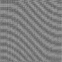
(a)	(b)
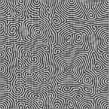
(c)	(d)

FIG. 2.: Instantaneous patterns of $\psi({\bf r},t)$ and $\omega_{z}({\bf r},t)$. Dark regions correspond to $\psi({\bf r},t)>0$ or $\omega_{z}({\bf r},t)>0$ while white regions to $\psi({\bf r},t)<0$ or $\omega_{z}({\bf r},t)<0$. (a) $\psi({\bf r},t)$ and (b) $\omega({\bf r},t)$ at $\epsilon=0.2$ on the roll branch; (c) $\psi({\bf r},t)$ and (d) $\omega({\bf r},t)$ at $\epsilon=0.65$ on the SDC branch.

The patterns we observed are very similar to those found in real experiments [6, 7], which can be summarized as the following: (A) Within the roll branch: Straight parallel rolls are observed at $\epsilon=0.05$ up to $0.4$ with a few defects at the boundary. Starting at $\epsilon=0.45$ up to $0.6$, the rolls start to bend and focal singularities start to appear near the boundary. Weak time-dependence sets in at $\epsilon=0.45$ in which the nucleation of defects along the sidewall occurs. Two typical shadow graph images, one for the order parameter $\psi({\bf r},t)$ and another for the vertical vorticity $\omega_{z}({\bf r},t)=-{{\bf\nabla}}^{2}\zeta({\bf r},t)$, of the roll state at $\epsilon=0.2$ are shown in Fig. 2. (B) Within the SDC branch: SDC states are observed at $\epsilon=0.8$ to $0.55$, whose behavior has been described in detail before [6, 7, 16]. At $\epsilon=0.5$, only a few spirals still exist which mix with a background of locally curved rolls. Finally at $\epsilon=0.4$, the pattern looks much like a roll state with a few defects and dislocations. In Fig. 2, we plot two typical shadow graph images, again one for $\psi({\bf r},t)$ and another for $\omega_{z}({\bf r},t)$, of SDC at $\epsilon=0.65$. While the vertical vorticity $\omega_{z}({\bf r})$ in a roll state is almost zero everywhere, the corresponding field has a much richer structure in SDC. This suggests choosing $\omega_{z}({\bf r},t)$ to be an order parameter in distinguishing a roll state from a SDC state [16]. It is interesting to point out that patterns in the interval $\epsilon=0.4-0.6$ depend on their earlier histories, i.e., whether they are on the roll branch or the SDC branch; see Fig. 3. So a hysteretic loop exists when one follows the two different routes. This is consistent with experimental observations that different patterns evolve from different initial conditions at the same $\epsilon$ [13]. Owing to the existence of hysteresis, the transition temperature $\epsilon_{T}$ between parallel roll states and SDC states cannot be determined precisely in our study. Our rough estimate is $\epsilon_{T}\simeq 0.45$.

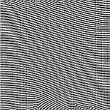
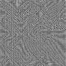
(a)	(b)

FIG. 3.: Instantaneous patterns of $\psi({\bf r},t)$ at $\epsilon=0.55$: (a) on the roll branch and (b) on the SDC branch. Dark regions correspond to $\psi({\bf r},t)>0$ while white regions to $\psi({\bf r},t)<0$.

In order to determine the character of the transition between rolls and SDC, we have calculated, from our numerical studies, the structure factor $S(k)$, the two-point correlation length $\xi_{2}$, the convective current $J$, the vorticity current $\Omega$, and the spectra entropy $\Xi$ for both roll states and SDC states. The numerical methods used in calculating these quantities are the same as in Ref. [16]. The numerical uncertainties are taken as the variances of our data. Considering that we can, at most, take just a few samples of the strongly fluctuating instantaneous quantities, presumingly obeying Gaussian distributions near their corresponding time-averaged values, we believe that the probabilities, and hence the uncertainties, for us to obtain the truly time-averaged values are determined by those variances. From the data for $S(k)$ of the SDC states, we have verified the existence of the scaling form (9) within our numerical uncertainties for SDC [15]. The results for $\xi_{2}$, $J$, $\Omega$ and $\Xi$ are plotted in Figs. 4 - 7. The most striking feature in these figures is the hysteretic loops formed by the two branches. It is also noticeable that the uncertainties on the SDC branch are generally larger than those on the roll branch, which, presumably, is due to the chaotic character of SDC.

We fit the data on the roll branch with power-law behaviors. To allow for the possibility that roll states might be unstable or metastable for $\epsilon>0.45$, only data for $0.05\leq\epsilon\leq 0.45$ are used in actual fittings. (i) We first use the nonlinear $\chi^{2}$ method to fit the convective current with $J=J_{0}(\epsilon-\epsilon_{c})^{\mu}$ and find that $J_{0}=0.6554\pm 0.0002$, $\mu=1.0054\pm 0.0004$ and $\epsilon_{c}=0.002$. The actual accuracy in our results may not as good as indicated. The fitting error for $\epsilon_{c}$ is very small. This $\epsilon_{c}$ is the measured onset from conduction to convection, whose positive value is most likely due to finite-size effects [27]. Apparently $J$ on the roll branch has a mean-field exponent. The amplitude $J_{0}$ is also in good agreement with Eq. (12) provided that $\langle x^{2}\rangle_{x}\geq 1$ is not too big. (ii) Using the $\chi^{2}$ method, we fit the data for the correlation length with $\xi_{2}=\xi_{2,0}(\epsilon-\epsilon_{c})^{-\nu}$, which leads to $\xi_{2,0}=13.0\pm 0.2$ and $\nu=0.54\pm 0.01$. So $\xi_{2}$ on the roll branch also has a mean-field exponent. (iii) Using the $\chi^{2}$ method, we fit the data for the vorticity current with $\Omega=\Omega_{0}(\epsilon-\epsilon_{c})^{\lambda}$ and find that $\Omega_{0}=(1.952\pm 0.008)\times 10^{-9}$ and $\lambda=2.461\pm 0.003$. Again, the actual accuracy in our results may not as good as indicated. This behavior of $\Omega$ is not easy to understand. The amplitude equations coupled with mean-flow predict, for rigid-rigid boundaries, that $\Omega\sim\epsilon^{7/2}$ for almost perfect parallel rolls and $\Omega\sim\epsilon^{3}$ for general patterns [19]. None of these can explain the behavior of $\Omega$ we found, which seems to be consistent with $\Omega\sim\epsilon^{5/2}$. (iv) The analysis of the spectra entropy is most difficult since there is no theory whatsoever to describe its behavior. We simply fit it to a form $\Xi=\Xi_{b}+\Xi_{0}(\epsilon-\epsilon_{c})^{\delta}$ for the roll states. We find from the nonlinear $\chi^{2}$ method that $\Xi_{b}=4.24\pm 0.04$, $\Xi_{0}=2.5\pm 0.1$ and $\delta=1.00\pm 0.08$. The background term $\Xi_{b}$ is much larger than the corresponding value for perfect parallel rolls $\Xi_{b}=\ln 2=0.6931$. This, presumably, is due to finite-size effects and/or limited computing time. The original data and their corresponding fitting curves for these global quantities are plotted in Figs. 4 - 7.

The analyses of the data on the SDC branch must be treated with caution given that there are three possible scaling scenarios as discussed in Sec. III. We first fit the data of $\xi_{2}$ and $\Omega$ to power laws such as (i) $\xi_{2}=\xi_{2,0}(\epsilon-\epsilon_{0})^{-\nu}$ and (ii) $\Omega=\Omega_{0}(\epsilon-\epsilon_{0})^{\lambda}$, where $\epsilon_{0}=\epsilon_{c}$ [the onset temperature in a finite system] in scenario (A) or $\epsilon_{0}=\epsilon_{T}$ [the roll-to-SDC transition temperature] in scenario (B). Then we fit the data of $J$ in accordance with our theoretical result in Eq. (10), i.e., (iii) $J=J_{0}(\epsilon-\epsilon_{c})-J_{\xi}\xi_{2}^{-2}$, where we take the corresponding fitting results for $\xi_{2}$ in (i). Clearly the value of $\epsilon_{0}$ is essential to determine which of the three scenarios is valid. In the following, we apply three different fittings for three values of $\epsilon_{0}$ and check the consistence of our numerical data against the theoretical results in Eqs. (10) and (11).

(a) To check whether scenario (A), i.e., ${\tilde{\epsilon}}=\epsilon$, is valid, we fix $\epsilon_{0}=\epsilon_{c}=0.002$, whose value is given by the fitting of $J$ on the roll branch. Since it is probable that SDC states are unstable or metastable at $\epsilon=0.4$ and $0.45$, the corresponding data might deviate from their “real” values in order to form the hysteretic loops. For this reason, we disregard these two points and use only those data within $0.5\leq\epsilon\leq 0.8$ for fitting. We use the $\chi^{2}$ method to fit our data, which leads to (i) $\xi_{0}=6.8\pm 0.2$ and $\nu=0.72\pm 0.05$; (ii) $\Omega_{0}=(3.0\pm 0.2)\times 10^{-8}$ and $\lambda=3.0\pm 0.1$; and (iii) $J_{0}=0.64\pm 0.02$ and $J_{\xi}=2.9\pm 0.9$. The original data of $\xi_{2}$, $J$ and $\Omega$ and their corresponding fitting curves are plotted in Fig. 4. Apparently those curves fit the original data well. So scenario (A) is consistent with our numerical data. To further distinguish scenario (A1) [$\nu=\frac{1}{2}$] or (A2) [$\nu>\frac{1}{2}$], we find that, on the one hand, $\nu=0.72\pm 0.05$ from the direct fitting in (i) but, on the other hand, $\nu=0.50\pm 0.05$ from $\lambda=3.0\pm 0.1$ in (ii) and $\lambda=2+2\nu$ in Eq. (20). This discrepancy is likely caused by the big numerical uncertainties in our data. We feel that the direct fitting is more reliable and scenario (A2) is more likely to be true. But we cannot definitely rule out scenario (A1). More accurate data are needed to resolve this issue.

(b) We check whether scenario (B), i.e., ${\tilde{\epsilon}}=\epsilon-\epsilon_{T}$, is consistent with our numerical data, where the value of $\epsilon_{T}$ is determined by the fitting of $\xi_{2}$. In contrast to case (a), there is no obvious reason to disregard any point in this scenario. So all the data within $0.4\leq\epsilon\leq 0.8$ are used in our fittings. We first use the nonlinear $\chi^{2}$ method to fit the data of $\xi_{2}$, which gives (i) $\xi_{0}=5.9\pm 0.2$, $\nu=0.46\pm 0.06$ and $\epsilon_{0}=\epsilon_{T}=0.27\pm 0.03$. Then, we fix $\epsilon_{0}=0.27$ and use the $\chi^{2}$ method to fit the data of $\Omega$ and $J$. We find that (ii) $\Omega_{0}=(8.1\pm 0.2)\times 10^{-8}$ and $\lambda=2.33\pm 0.01$; and (iii) $J_{0}=0.675\pm 0.001$ and $J_{\xi}=4.9\pm 0.1$. These results are very sensitive to the points at $\epsilon=0.4$ and $0.45$. The original data of $\xi_{2}$, $J$ and $\Omega$ and their corresponding fitting curves are plotted in Fig. 5. The fitting of $\Omega$ obviously is not good. The results $\nu=0.46\pm 0.06$ in (i) and $\lambda=2.33\pm 0.01$ in (ii) do not satisfy the scaling relation $\lambda=2\nu$ in Eq. (27). So scenario (B) with $\epsilon_{T}=0.27$ is unlikely to be true.

(c) We check whether scenario (B), with $\epsilon_{T}$ determined by the fitting of $\Omega$, is consistent with our numerical data. As in case (b), we use all the data within $0.4\leq\epsilon\leq 0.8$ in our fittings. We first use the nonlinear $\chi^{2}$ method to fit the data of $\Omega$ and find that (ii) $\Omega_{0}=(4.5\pm 0.3)\times 10^{-8}$, $\lambda=1.41\pm 0.07$ and $\epsilon_{T}=0.348\pm 0.005$. Then we fix $\epsilon_{0}=0.348$ and apply the $\chi^{2}$ method to fit the data of $\xi_{2}$ and $J$. We find that (i) $\xi_{2,0}=6.55\pm 0.09$ and $\nu=0.295\pm 0.008$; and (iii) $J_{0}=0.667\pm 0.001$ and $J_{\xi}=4.6\pm 0.1$. Again, these fitting results are very sensitive to the points at $\epsilon=0.4$ and $0.45$. The original data of $\xi_{2}$, $J$ and $\Omega$ and their corresponding fitting curves are plotted in Fig. 6. Notice that, since $\nu$ in (i) is less than $\frac{1}{2}$, the slope of $J$ is negative in the range of $0<{\tilde{\epsilon}}=\epsilon-\epsilon_{T}<{\tilde{\epsilon}}_{\times}$ with ${\tilde{\epsilon}}_{\times}=[2\nu J_{\xi}/\xi_{2,0}^{2}J_{0}]^{1/(1-2\nu)}$. In the present case, one has ${\tilde{\epsilon}}_{\times}=3.20\times 10^{-3}$, which perhaps is too small to be checked by real experiments or simulations. From the pure-data-fitting point of view, the fittings in this case are as good as the fittings in case (a). So, without the benefit of our theoretical results, scenario (B) with $\epsilon_{T}=0.348$ could be (incorrectly) accepted. But, the exponents $\nu=0.295\pm 0.008$ in (i) and $\lambda=1.41\pm 0.07$ in (ii) are not even close to satisfying the scaling relation $\lambda=2\nu$ in Eq. (27). So this scenario can be ruled out by our theory. From this, together with the discussions in case (a) and (b), we conclude that scenario (B) is unlikely to be valid for SDC and scenario (A) is consistent with our numerical data and our theory.

$\xi_{2}^{-2}$

$J$

$10^{9}\Omega$

$\epsilon$

FIG. 4.: Plots of $\xi_{2}^{-2}$, $J$ and $\Omega$ vs. $\epsilon$ for both parallel rolls and SDC. The corresponding fitting curves for SDC are described in (a) in Sec. IV. The labels are used as the following: SDC — the numerical data with error bars on the SDC branch; (a) — the fitting curves for SDC described in (a) in the text; Roll — the numerical data with error bars on the roll branch; (p) — the fitting curves for parallel rolls. To indicate the parallel roll states for $\epsilon>\epsilon_{T}$ and the SDC states for $\epsilon<\epsilon_{T}$ may be metastable, the corresponding fitting curves in (a) and (p) are plotted with dotted lines. The transition temperature is estimated roughly at $\epsilon_{T}=0.45$.

It is worthwhile to mention that, in all cases above, the value of $J_{0}$ agrees with the theoretical result $2/3$ in Eq. (10); the value of $J_{\xi}$ is also consistent with the theoretical prediction $J_{\xi}\geq 8/3$. On the other hand, the theoretical results in Eqs. (22) and (29) predict that $\Omega_{0}=7.4\times 10^{-4}$ in case (a), $\Omega_{0}=7.2\times 10^{-5}$ in case (b), and $\Omega_{0}=9.7\times 10^{-5}$ in case (c). All these predictions are several orders larger than the corresponding numerical results. The reason for such big discrepancies is not clear to us.

We have also studied the behavior of the spectra entropy. Owing to the lack of any theory, we simply fit the data of $\Xi$ to a form $\Xi=\Xi_{b}+\Xi_{0}(\epsilon-\epsilon_{0})^{\delta}$ for the SDC branch. We apply two different fittings: (a) We fix $\epsilon_{0}=\epsilon_{c}$ and $\Xi_{b}=4.24$ [from the fitting for the roll branch], and use the $\chi^{2}$ method to fit those data within $0.5\leq\epsilon\leq 0.8$, which leads to $\Xi_{0}=4.79\pm 0.03$ and $\delta=0.18\pm 0.02$. (b) We fix $\Xi_{b}=4.24$ and use the nonlinear $\chi^{2}$ method for all data within $0.4\leq\epsilon\leq 0.8$, which gives that $\Xi_{0}=5.13\pm 0.05$, $\delta=0.12\pm 0.01$ and $\epsilon_{0}=0.37\pm 0.02$. We have also tried other alternative fittings such as using the nonlinear $\chi^{2}$ method for all data within $0.4\leq\epsilon\leq 0.8$ and fixing $\epsilon_{0}=0.27$ [from (i) in (b)] or $\epsilon_{0}=0.348$ [from (ii) in (c)], but none of them gives a reasonable fit. The fitting curves in (a) and (b) and the original data of $\Xi$ are plotted in Fig. 7. At this stage, the behavior of $\Xi$ is the most unclear one among all the time-averaged global quantities defined in Sec. II.

$\xi_{2}^{-2}$

$J$

$10^{9}\Omega$

$\epsilon$

FIG. 5.: Plots of $\xi_{2}^{-2}$, $J$ and $\Omega$ vs. $\epsilon$ for both parallel rolls and SDC. The corresponding fitting curves for SDC are described in (b) in Sec. IV. The labels are used as the following: SDC — the numerical data with error bars on the SDC branch; (b) — the fitting curves for SDC described in (b) in the text; Roll — the numerical data with error bars on the roll branch; (p) — the fitting curves for parallel rolls.

$\xi_{2}^{-2}$

$J$

$10^{9}\Omega$

$\epsilon$

FIG. 6.: Plots of $\xi_{2}^{-2}$, $J$ and $\Omega$ vs. $\epsilon$ for both parallel rolls and SDC. The corresponding fitting curves for SDC are described in (c) in Sec. IV. The labels are used as the following: SDC — the numerical data with error bars on the SDC branch; (c) — the fitting curves for SDC described in (c) in the text; Roll — the numerical data with error bars on the roll branch; (p) — the fitting curves for parallel rolls.

V Discussion and Conclusion

In the previous section, we conclude that scenario (A) is valid for SDC. This means that $\xi_{2}$ diverges at $\epsilon=0$, and $J$ and $\Omega$ vanish at $\epsilon=0$. At first sight it seems puzzling that all properties of SDC are controlled by $\epsilon$, instead of $\epsilon-\epsilon_{T}$. To understand this, we propose an explanation for this scenario, which is somewhat similar to that in the hexagon-to-roll transition in non-Boussinesq fluids [21]. In the latter case, the transition from hexagonal states to parallel roll states occurs at finite $\epsilon_{T}$. Although the roll attractor is unstable for small enough $\epsilon$ and metastable against the hexagonal attractor for even slightly larger $\epsilon$, the properties of the parallel roll states are all controlled by $\epsilon$, not by $\epsilon-\epsilon_{T}$ [21]. Clearly one can imagine a similar picture for the roll-to-SDC transition. While the SDC attractor seems to be either unstable or metastable against the roll attractor for sufficiently small $\epsilon$, as an intrinsic convective state, the properties of SDC are controlled at the conduction to convection threshold, not where it starts to emerge as the stable state. The existence of two different attractors has been suggested by experiments [12, 13]. The basins and the stability of these two attractors are still unclear at present.

$\Xi$

$\epsilon$

FIG. 7.: Plot of $\Xi$ vs. $\epsilon$ for both parallel rolls and SDC. The different fitting forms (a) and (b) for SDC are discussed in the text. The labels are used as the following: Roll — the numerical data with error bars on the roll branch; SDC — the numerical data with error bars on the SDC branch; (a) — the fitting curve for SDC described in (a) in the text; (b) — the fitting curve for SDC described in (b) in the text; (p) — the fitting curve for parallel rolls. To indicate the parallel roll states for $\epsilon>\epsilon_{T}$ and the SDC states for $\epsilon<\epsilon_{T}$ may be metastable, the corresponding fitting curves in (a) and (p) are plotted with dotted lines. The transition temperature is estimated roughly at $\epsilon_{T}=0.45$.

The establishment of scenario (A) indicates that the transition between the parallel roll states and the SDC states is first-order. This conclusion is also supported by the following:

(1) Our theory predicts discontinuities in the value and the slope of $J$ at $\epsilon_{T}$ [see the discussion following Eq. (16)]. This is a typical signature of a first-order transition.

(2) The presence of hysteretic loops in Figs. 4 - 7 is a strong indication of a first-order transition. A different hysteretic loop has also been reported by others for the GSH model [14]. Although it is arguable that hysteretic loops may be found in a second-order transition if the computing time is not long enough to overcome the effects of critical slowing-down (which occurs when the correlation time $\tau$ approaches infinity), it is doubtful that the loops in that case can be as distinctive as what we found in Figs. 4 - 7.

(3) As we described in Sec. IV, the convective patterns depend on the processes leading to them, which is also observed in experiments [13]. This fact suggests that the two competing attractors are either both stable or one is stable while the other is metastable for some positive $\epsilon$. Such a stability property is typical in first-order transitions. On the contrary, in second-order transitions one of the two attractors should change from stable to unstable while the other changes from unstable to stable as $\epsilon$ moves across $\epsilon_{T}$.

(4) From Figs. 5 - 7, it is easy to see that, if scenario (B) is valid, then the fitting curves of all the time-averaged global quantities on the SDC branch will cross those on the roll branch. But there is no evidence from our numerical calculation supporting such a crossing.

As we mentioned in Sec. I, an earlier experiment with a circular cell [12] found that $\xi_{2}$ diverges at $\epsilon=0$ with a mean-field exponent, while the correlation time $\tau$ either diverges at $\epsilon=0$ with a non-mean-field exponent or diverges at the roll-to-SDC transition temperature $\epsilon_{T}$ with a mean-field exponent. However, a recent experiment with a square cell [13] concluded that $\xi_{2}$ diverges at $\epsilon_{T}$ with a very small exponent $\nu$. We now comment on these experiments and our study.

Regarding our numerical study, we cannot rule out that the roll-to-SDC transition in the GSH model has a different character from those in real experiments although this seems unlikely. We also cannot rule out that our numerical solutions are still in the transient regime even though we have waited for about four horizontal diffusion times $t_{h}$ before collecting data over an interval of several $t_{h}$ for each $\epsilon$. Furthermore, as we discussed in Sec. IV, our numerical data are not accurate enough to determine independently which of the three scenarios is true for SDC. As a result, we have to rely on our theoretical predictions to resolve this issue. Finally we disregarded two data points in our analysis for scenario (A) on the basis that these two points deviate from their “real” values to form hysteretic loops. This introduces a certain arbitrariness in determining which data points deviate. These shortcomings in our numerical study weaken the validity of our conclusion.

We notice that the data of the correlation length $\xi_{2}$ for parallel rolls and SDC were analyzed together in the experiment by Morris et al. [12], which we think is not justified. Considering that the parallel roll states and the SDC states are intrinsically different, we believe it is necessary to separate their data in the analysis, such as we did in Sec. IV. Such a separation was implicit for the data of the correlation time $\tau$ since $\tau=+\infty$ for steady states such as parallel rolls and, in principle, only the data for SDC are available. A divergence at $\epsilon=0$ with a non-mean-field exponent was found to be consistent with the data of $\tau$ for SDC [12]. It is not clear to us whether a similar conclusion can be reached for $\xi_{2}$ if its data for SDC are analyzed separately.

The conclusion by Cakmur et al. [13] that $\xi_{2}$ diverges at $\epsilon_{T}$ with a small exponent $\nu$ is different from that in Ref. [12] and ours. These authors suggested that the different geometry of experimental cells is the cause for the different results between theirs and that in Ref. [12]. If so, then it is not clear to us what the real behavior is in an infinite system. In our calculation, we also used a square cell. We think that there may exist a different interpretation of the experimental data for $\xi_{2}$ obtained in Ref. [13]. We believe that, to convincingly show that $\xi_{2}$ for SDC diverges at $\epsilon_{T}$, one must have sufficient data points whose $\xi_{2}$ are much larger than the corresponding typical values of parallel rolls (for $\epsilon$ away from both $0$ and $\epsilon_{T}$). Otherwise, the data for $\xi_{2}$ for SDC may simply approach those for parallel rolls to form a hysteretic loop near $\epsilon_{T}$, instead of diverging at $\epsilon_{T}$. Since no data for $\xi_{2}$ for the parallel roll states was given and the number of data for SDC near $\epsilon_{T}$ was relatively limited, we feel the conclusion by Cakmur et al. [13] should be treated with caution.

As we discussed in Sec. IV, our theory plays an important role in determining the nature of the roll-to-SDC transition. So it is very important to check our theoretical predictions by real experiments. One important prediction by our theory is that there exist discontinuities in the value and the slope of $J$ at $\epsilon_{T}$. However, we realize that no discontinuity in $J$ has been reported by experiments. The reason for this is not clear to us. We conjecture that finite size effects might play a role. From Fig. 1, we find that the discontinuity is larger for smaller Prandtl number $\sigma$. So it would be interesting to see whether experiments can confirm or rule out such a discontinuity in $J$ by using a small $\sigma$. Another important prediction from our analysis is the behavior of the time-averaged vorticity current $\Omega$. Since direct measurements of $\Omega$ seem to be very difficult in real experiments [28], we think it valuable to calculate $\Omega$ by solving Eq. (2) [the corresponding version before rescalings can be found in Ref. [15]] or its improved versions numerically, with the experimental results of $\psi({\bf r},t)$ as input. Such a calculation will not only help to clarify the nature of the roll-to-SDC transition, but also provide an additional experimental test on our theory [15]. It would also be useful to calculate the time-averaged spectra entropy as suggested in Refs. [13, 16], even though there is no theory to predict the behavior of this quantity.

In summary, we conclude from our numerical studies and our theoretical results that the roll-to-SDC transition is first-order in character. We found that the correlation length $\xi_{2}$ for SDC diverges at $\epsilon=0$, not at the transition temperature $\epsilon_{T}$. However, since the uncertainties in our data are unpleasantly large and the data points we have are unsatisfactorily few in number, we cannot determine definitely whether the exponent of $\xi_{2}$ is mean-field or not. So further investigations are necessary to draw a definite conclusion. In this regard, a theoretical calculation of $\xi_{2}$ for SDC is highly desirable. A theory to describe the roll-to-SDC transition is essential. Finite size effects should also be studied carefully.

Acknowledgment

X.J.L and J.D.G are supported by the National Science Foundation under Grant No. DMR-9596202. H.W.X. is supported by the Research Corporation under Grant No. CC4250. Numerical work reported here was carried out on the Cray-C90 at the Pittsburgh Supercomputing Center and Cray-YMP8 at the Ohio Supercomputer Center.

REFERENCES

- [1]
- [2] For a recent review on pattern formation in various systems, see: M. C. Cross and P. C. Hohenberg, Rev. Mod. Phys. 65, 851 (1993).
- [3] H. S. Greenside, chao-dyn/9612004.
- [4] G. Ahlers, in 25 Years of Nonequilibrium Statistical Mechanics, edited by J. J. Brey et al. (Springer, New York, 1995), p. 91.
- [5] A. Schlüter, D. Lortz, and F. Busse, J. Fluid Mech. 23, 129 (1965); F. H. Busse, Rep. Prog. Phys. 41, 1929 (1978); F. H. Busse and R. M. Clever, in New Trends in Nonlinear Dynamics and Pattern-Forming Phenomena, edited by P. Coullet and P. Huerre (Plenum Press, New York, 1990), p. 37; and references therein.
- [6] S. W. Morris, E. Bodenschatz, D. S. Cannell and G. Ahlers, Phys. Rev. Lett. 71, 2026 (1993).
- [7] M. Assenheimer and V. Steinberg, Phys. Rev. Lett. 70, 3888 (1993); Nature 367, 345 (1994).
- [8] H.-W. Xi, J. D. Gunton and J. Viñals, Phys. Rev. Lett. 71, 2030 (1993).
- [9] M. Bestehorn, M. Fantz, R. Friedrich, and H. Haken, Phys. Lett. A 174, 48 (1993).
- [10] W. Decker, W. Pesch and A. Weber, Phys. Rev. Lett. 73, 648 (1994).
- [11] Y. Hu, R. E. Ecke and G. Ahlers, Phys. Rev. Letts. 74, 391 (1995); J. Liu and G. Ahlers, ibid 77, 3126 (1996).
- [12] S. W. Morris, E. Bodenschatz, D. S. Cannell, and G. Ahlers, Physica D 97, 164 (1996).
- [13] R. V. Cakmur, D. A. Egolf, B. B. Plapp, and E. Bodenschatz, patt-sol/9702003.
- [14] M. C. Cross and Y. Tu, Phys. Rev. Lett. 75, 834 (1995).
- [15] X.-J. Li, H.-W. Xi, and J. D. Gunton, patt-sol/9706007.
- [16] H.-W. Xi and J. D. Gunton, Phys. Rev. E 52, 4963 (1995). A factor of was missed for the quantity there.
- [17] J. Swift and P. C. Hohenberg, Phys. Rev. A 15, 319 (1977).
- [18] M. C. Cross, Phys. Fluids 23, 1727 (1980); G. Ahlers, M. C. Cross, P. C. Hohenberg, and S. Safran, J. Fluid Mech. 110, 297 (1981).
- [19] E. D. Siggia and A. Zippelius, Phys. Rev. Lett. 47, 835 (1981); M. C. Cross, Phys. Rev. A 27, 490 (1983); P. Manneville, J. Phys. (Paris) 44, 759 (1983).
- [20] G. C. Powell and I. C. Percival, J. Phys. A 12, 2053 (1979).
- [21] F. H. Busse, J. Fluid Mech. 30, 625 (1967); C. Pérez-García, E. Pampaloni and S. Ciliberto, in Quantitative Measures of Complex Dynamical Systems, edited by N. B. Abraham and A. Albano (Plenum, New York, 1990), p. 405; E. Pampaloni, C. Pérez-García, L. Albavetti and S. Ciliberto, J. Fluid Mech. 234, 393 (1992).
- [22] H.-W. Xi, J. Viñals and J. D. Gunton, Phys. Rev. A 46, R4483 (1992); H.-W. Xi, J. D. Gunton and J. Viñals, Phys. Rev. E 47, R2987 (1993); X.-J. Li, H.-W. Xi, and J. D. Gunton, ibid 54, R3105 (1996).
- [23] H. S. Greenside and M. C. Cross, Phys. Rev. A 31, 2492 (1985).
- [24] F. H. Busse, in Advances in Turbulence 2, Edited by H.-H. Fernholz and H. E. Fiedler (Springer-Verlag, Berlin, 1989); F. H. Busse, M. Kropp, and M. Zaks, Physica D 61, 94 (1992).
- [25] H.-W. Xi, X.-J. Li, and J. D. Gunton, Phys. Rev. Lett. 78, 1046 (1997); and [to be submitted].
- [26] P. E. Bjørstad et al., in Elliptic Problem Solvers II, Edited by G. Birkhoff and A. Schoenstadt (Academic, Orlando, 1984), p. 531; H.S. Greenside and W.M. Coughran Jr., Phys. Rev. A 30, 398 (1984).
- [27] R. W. Walden and G. Ahlers, J. Fluid Mech. 109, 89 (1981); R. P. Behringer and G. Ahlers, ibid 125, 219 (1982).
- [28] V. Croquette, P. Le Gal, and Pocheau, Europhys. Lett. 1, 393 (1986); F. Daviaud and A. Pocheau, ibid 9, 675 (1989).