[

The Dynamics of Curved Fronts: Beyond Geometry

Abstract

We derive a new set of kinematic equations for front motion in two-dimensional bistable media. The equations generalize the geometric approach by complementing the equation for the front curvature with an order parameter equation associated with a nonequilibrium Ising-Bloch bifurcation. The resulting equations capture the core structure of spiral waves and spontaneous spiral-wave nucleation.

]

Traveling wave phenomena in reaction-diffusion systems often involve sharp interfaces or fronts separating different reaction states. The dynamics of two-dimensional sharp fronts has been studied successfully using a geometric approach [3, 4, 5, 6, 7]. Given a relation between the normal velocity of the front and its curvature, the geometric theory consists of a closed integro-differential equation for the front curvature from which the front line shape in the physical plane can be extracted. Inherent in this approach is the assumption that the inner front structure does not change significantly in time. This assumption rules out major changes like spontaneous nucleation of spiral waves along the front. Such phenomena have been observed recently in numerical simulations of model equations describing bistable reaction-diffusion systems. Very often the nucleation of spiral waves triggers spot replication and spiral turbulence [8, 9, 10, 11].

In this Letter we present a new kinematic approach for front motion in two-dimensional bistable media that captures spontaneous spiral-wave nucleation along the front. A key step in this approach is the consideration of a parameter range including a nonequilibrium Ising-Bloch (NIB) front bifurcation. This parity breaking bifurcation renders a stationary planar front unstable and gives rise to a pair of stable counter-propagating fronts. The bifurcation has been found in a number of models, including the forced complex Ginzburg-Landau [12] and FitzHugh-Nagumo [13, 14, 15] equations, and in experiments with chemical reactions [16] and liquid crystals [17].

Our kinematic approach consists of three equations:

• A geometric equation for the front curvature, $\kappa$:

  $${\partial\kappa\over\partial t}=-(\kappa^{2}+{\partial^{2}\over\partial s^{2}})C_{n}-{\partial\kappa\over\partial s}\int_{0}^{s}\kappa C_{n}ds^{\prime}\,.$$ (1)

• An equation relating the normal front velocity $C_{n}$, the curvature $\kappa$, and the order parameter, $C_{0}$, associated with the NIB bifurcation:

  $$C_{n}=C_{0}-D\kappa\,.$$ (2)

• An equation for the order parameter:

  $${\partial C_{0}\over\partial t} = (\alpha_{c}-\alpha)C_{0}-\beta C_{0}^{3}+\gamma\kappa+\gamma_{0}$$ (4)

  $$\mbox{}+{\partial^{2}C_{0}\over\partial s^{2}}-{\partial C_{0}\over\partial s}\int_{0}^{s}\kappa C_{n}ds^{\prime}\,.$$

In these equations $s$ is the front arclength, and the critical parameter value $\alpha_{c}$ designates the NIB bifurcation point. Notice that $C_{0}$ coincides with the planar front velocity when $\kappa=0$.

The curvature equation (1) together with the eikonal equation (2), where $C_{0}$ is considered constant, constitute the geometric approach used in earlier studies [4, 6]. Relaxing the requirement of constant $C_{0}$ by adding Eq. (4) allows for spontaneous local reversal of the direction of front propagation. The reversals are accompanied by the nucleation of spiral-wave pairs. In the rest of this Letter we describe the derivation of Eqs. (2) and (4) for a particular model and use these equations to demonstrate a mechanism of spontaneous spiral-wave nucleation.

We consider the FitzHugh-Nagumo model with a diffusing inhibitor,

$${\partial u\over\partial t} = \epsilon^{-1}(u-u^{3}-v)+\delta^{-1}\nabla^{2}u\,,$$ (5)

$${\partial v\over\partial t} = u-a_{1}v-a_{0}+\nabla^{2}v\,,$$ (6)

where $u$ and $v$, the activator and the inhibitor, are real scalar fields and $\nabla^{2}$ is the Laplacian operator in two dimensions. The parameter $a_{1}$ is chosen so that (6) describes a bistable medium having two stable uniform states: an “up” state $(u_{+},v_{+})$ and a “down” state $(u_{-},v_{-})$. Ising and Bloch front solutions connect the two uniform states $(u_{\pm},v_{\pm})$ as the spatial coordinate normal to the front goes from $-\infty$ to $+\infty$. The parameter space of interest is spanned by $\epsilon,\delta$ and $a_{0}$, or alternatively by $\eta=\sqrt{\epsilon\delta}$, $\mu=\epsilon/\delta$, and $a_{0}$. Note the parity symmetry $(u,v)\to(-u,-v)$ of (6) for $a_{0}=0$.

The NIB bifurcation line for $a_{0}=0$ is shown in Fig. 1. For $\mu\ll 1$ it is given by $\delta=\delta_{F}(\epsilon)=\eta_{c}^{2}/\epsilon$, or $\eta=\eta_{c}$, where $\eta_{c}=\frac{3}{2\sqrt{2}q^{3}}$ and $q^{2}=a_{1}+1/2$ [14]. The single stationary Ising front that exists for $\eta>\eta_{c}$ loses stability to a pair of counter-propagating Bloch fronts at $\eta=\eta_{c}$. Beyond the bifurcation ($\eta<\eta_{c}$) a Bloch front pertaining to an up state invading a down state coexists with another Bloch front pertaining to a down state invading an up state. Also shown in Fig. 1 are the transverse instability boundaries (for $a_{0}=0$), $\delta=\delta_{I}(\epsilon)=\epsilon/\eta_{c}^{2}$ and $\delta=\delta_{B}(\epsilon)=\eta_{c}/\sqrt{\epsilon}$, for Ising and Bloch fronts respectively. Above these lines, $\delta>\delta_{I,B}$, planar fronts are unstable to transverse perturbations [9, 10]. All three lines meet at a codimension 3 point $P3$: $\epsilon=\eta_{c}^{2}$, $\delta=1$, $a_{0}=0$.

FIG. 1.: The NIB front bifurcation and transverse instability boundaries. The thick line is the NIB bifurcation, $\delta(\epsilon)$, and the dashed lines are the boundaries for transverse instability of Ising, $\delta_{I}(\epsilon)$, and Bloch, $\delta(\epsilon)$, fronts. The thin lines are the linear approximations to the transverse instability boundaries near the codimension 3 point, $P3$. Parameters: $a_{1}=4.0$, $a_{0}=0$.

The following assumptions are made to derive Eqs. (2) and (4): $\epsilon$ and $\delta$ are in the proximity of the codimension 3 point, $P3$, with $\epsilon<<1$; the radius of curvature is much larger than the front width, that is, $\kappa\ll q$. First, we transform to an orthogonal coordinate system $(r,s)$ that moves with the front, where $r$ is a coordinate normal to the front. Let ${\bf X}(s,t)=(X,Y)$ denote the position vector of the front. More precisely we identify ${\bf X}(s,t)$ with the $u=0$ contour line. The relation between the laboratory frame $(x,y)$ and the moving frame is

$$x=X(s,t)+r{\partial Y\over\partial s}\qquad y=Y(s,t)-r{\partial X\over\partial s}\,.$$ (7)

In the moving frame Eqs. (6) become

$$\epsilon{\cal D}u = u-u^{3}-v+\mu{\cal L}u\,,$$ (8)

$${\cal D}v = u-a_{1}v-a_{0}+{\cal L}v\,,$$ (9)

where

$${\cal D} = {\partial\over\partial t}+{\partial s\over\partial t}{\partial\over\partial s}+{\partial r\over\partial t}{\partial\over\partial r}\,,$$ (10)

$${\cal L} = {\partial^{2}\over\partial r^{2}}+\kappa F{\partial\over\partial r}+F{\partial F\over\partial s}{\partial\over\partial s}+F^{2}{\partial^{2}\over\partial s^{2}}\,,$$ (11)

$F=(1+r\kappa)^{-1}$, and the curvature is $\kappa={\partial X\over\partial s}{\partial^{2}Y\over\partial s^{2}}-{\partial Y\over\partial s}{\partial^{2}X\over\partial s^{2}}$ [18]. The change of the arclength in time is due to stretching and is given by [4, 6]

$${\partial s\over\partial t}=\int_{0}^{s}\kappa C_{n}ds^{\prime}\,.$$ (12)

Recalling that $\mu=\epsilon/\delta\ll 1$, we use singular perturbation theory and distinguish between an inner region where $\mu\frac{\partial^{2}u}{\partial r^{2}}\sim{\cal O}(1)$, and outer regions where $\mu{\partial^{2}u\over\partial r^{2}}\sim{\cal O}(\mu)$. The inner region pertains to the front core where the profile of $u$ in the normal direction is steep. Introducing a stretched coordinate $z=r/\sqrt{\mu}$ and expanding $u=u_{0}+\epsilon u_{1}+\epsilon^{2}u_{2}+\ldots$ and $v=v_{0}+\epsilon v_{1}+\epsilon^{2}v_{2}+\ldots\,$, we obtain at order unity $u_{0}=-\tanh z/\sqrt{2}$, $v_{0}=0$. At order $\epsilon$ the solvability condition is

$${\partial r\over\partial t}={3\over\eta\sqrt{2}}v_{f}+\delta^{-1}\kappa\ ,$$ (13)

where $v_{f}=v(0,s,t)+{\cal O}(\epsilon^{2})$ is the approximately constant value of the inhibitor $v$ in the narrow [${\cal O}(\sqrt{\mu})$] front core region. The first term on the right-hand-side of (13) is identified with the order parameter for the NIB bifurcation: $C_{0}=-{3\over\eta\sqrt{2}}v_{f}$. Since the normal velocity is $C_{n}=-{\partial r\over\partial t}$, Eq. (13) yields the eikonal equation (2) with $D=\delta^{-1}$.

In the outer regions ${\partial^{2}u\over\partial r^{2}}\sim{\cal O}(1)$ and the leading order equation for $u$ is $u-u^{3}-v=0$. The relevant solutions are $u=u_{+}(v)\approx 1-v/2$ for $r<0$ and $u=u_{-}(v)\approx-1-v/2$ for $r>0$ (assuming $a_{1}$ is sufficiently large) [14]. To leading order in $\epsilon$ we obtain for $v$ the free boundary problem

$$\left({\partial\over\partial t}-{\partial^{2}\over\partial r^{2}}+q^{2}\right)v = +1-{3\over\eta\sqrt{2}}v_{f}{\partial v\over\partial r}+P_{1}+P_{2},\quad r\leq 0$$ (14)

$$\left({\partial\over\partial t}-{\partial^{2}\over\partial r^{2}}+q^{2}\right)v = -1-{3\over\eta\sqrt{2}}v_{f}{\partial v\over\partial r}+P_{1}+P_{2},\quad r\geq 0$$ (15)

$$v(\mp\infty,s,t) = v_{\pm}={\pm 1-a_{0}\over q^{2}}\ ,$$ (16)

$$\left[v\right]_{r=0} = \left[{\partial v\over\partial r}\right]_{r=0}=0\ ,$$ (17)

where

$$P_{1} = (1-\delta^{-1})\kappa{\partial v\over\partial r}-a_{0}+F^{2}{\partial^{2}v\over\partial s^{2}}-{\partial s\over\partial t}{\partial v\over\partial s}\,,$$ (18)

$$P_{2} = F{\partial F\over\partial s}{\partial v\over\partial s}\,,$$ (19)

and the square brackets denote jumps of the quantities inside the brackets across the front at $r=0$.

To solve this free boundary problem we consider a parameter range in the immediate vicinity of the $P3$ point in Fig. 1. In that range the transverse instabilities of the fronts involve only small wavenumbers and therefore we can assume weak dependence of $v$ and $\kappa$ on the arclength $s$. In addition, the front speed is small and vanishes at $P3$. This suggests using the speed of a planar Bloch front solution, $c\propto\sqrt{\eta_{c}-\eta}$, as a small parameter. The weak dependence of $v$ and $\kappa$ on $s$ is achieved by introducing the slow length scale $S=cs$ and assuming ${\bf X}={\bf X}(S,t)$. This assumption dictates $\kappa=c^{3}\kappa_{0}$ where $\kappa_{0}\sim{\cal O}(1)$. We also introduce a slow time scale $T=c^{2}t$ to describe deviations from steady front motion.

Following Ref. [19], we solve the free boundary problem (17) by expanding propagating curved front solutions as power series in $c$ around the stationary planar Ising front

$$v(r,S,t,T)=v^{(0)}(r)+\sum_{n=1}^{\infty}c^{n}v^{(n)}(r,S,t,T)\ ,$$ (20)

where $v^{(0)}(r)=(1-e^{qr})/q^{2}$ for $r\leq 0$ and $v^{(0)}(r)=(e^{-qr}-1)/q^{2}$ for $r\geq 0$. Expanding $\eta=\eta_{c}-c^{2}\eta_{1}+c^{4}\eta_{2}+...$ and using these expansions in (17) produces the set of equations

$$\frac{\partial v^{(n)}}{\partial t}+q^{2}v^{(n)}-\frac{\partial^{2}v^{(n)}}{\partial r^{2}}=-\rho^{(n)},~{}n=1,2,3,\ldots$$ (21)

where $\rho^{(1)}$ and $\rho^{(2)}$ are as in Ref. [19] and $\rho^{(3)}$ is

$$\rho^{(3)}(r,S,t,T)={\partial v^{(1)}\over\partial T}+{3\eta_{1}\over\sqrt{2}\eta_{c}^{2}}v^{(1)}_{|r=0}{\partial v^{(0)}\over\partial r}$$ (24)

$$\mbox{}+{3\over\sqrt{2}\eta_{c}}\left[v^{(1)}_{|r=0}{\partial v^{(2)}\over\partial r}+v^{(2)}_{|r=0}{\partial v^{(1)}\over\partial r}+v^{(3)}_{|r=0}{\partial v^{(0)}\over\partial r}\right]+a_{00}$$

$$\mbox{}-F^{2}{\partial^{2}v^{(1)}\over\partial S^{2}}-(1-\delta^{-1})\kappa_{0}{\partial v^{(0)}\over\partial r}+{\partial S\over\partial T}{\partial v^{(1)}\over\partial S}\ .$$

In (24) we assumed $a_{0}=c^{3}a_{00}$ where $a_{00}\sim{\cal O}(1)$, and recall that $\kappa_{0}=\kappa/c^{3}$. Notice that ${\partial S\over\partial T}\sim{\cal O}(1)$, and $P_{2}$ contributes only at orders higher than $c^{3}$. We solve Eq. (21) using the asymptotic behavior of an appropriate Green’s function as in Ref. [19]. The results for $n=1,2$ remain unchanged and give the front bifurcation point $\eta_{c}={3\over 2\sqrt{2}q^{3}}$. The solution of (21) with $n=3$ yields the compatibility condition

$${\partial v^{(1)}\over\partial T} = {\sqrt{2}\eta_{1}\over q\eta_{c}^{2}}v^{(1)}-{3\over 4\eta_{c}^{2}}{v^{(1)}}^{3}-{4\over 3}a_{00}$$ (26)

$$\mbox{}-{2(1-\delta^{-1})\over 3q}\kappa_{0}+{\partial^{2}v^{(1)}\over\partial S^{2}}-{\partial S\over\partial T}{\partial v^{(1)}\over\partial S}\ ,$$

or expressing the slow time and arclength derivatives in terms of the fast variables $t,s$ and using (12) and (20),

$${\partial v_{f}\over\partial t} = {\sqrt{2}(\eta_{c}-\eta)\over q\eta_{c}^{2}}v_{f}-{3\over 4\eta_{c}^{2}}v_{f}^{3}-{4\over 3}a_{0}$$ (28)

$$\mbox{}-{2(1-\delta^{-1})\over 3q}\kappa+{\partial^{2}v_{f}\over\partial s^{2}}-{\partial v_{f}\over\partial s}\int_{0}^{s}\kappa C_{n}ds^{\prime}\ .$$

Equation (28) coincides with (4) once we make the following identifications: $C_{0}=-{3\over\eta\sqrt{2}}v_{f}$, $\alpha={\eta\sqrt{2}\over q\eta_{c}^{2}}$, $\alpha_{c}={\sqrt{2}\over q\eta_{c}}$, $\beta=1/6$, $\gamma=\alpha_{c}(1-\delta^{-1})$, and $\gamma_{0}=2\alpha_{c}qa_{0}$.

Equation (4) reproduces the NIB bifurcation for planar fronts: setting $\kappa=0$ and $a_{0}=0$ we find the Ising front branch $C_{0}=0$ and the two Bloch front branches $C_{0}=\pm\sqrt{(\alpha_{c}-\alpha)/\beta}$. To test whether Eqs. (1)-(4) also capture the transverse instabilities we check the linear stability of planar front solutions near the $P3$ point in the $a_{0}=0$ plane. Let $C_{0}=C_{0}^{0}+\bar{C}_{0}\exp(\sigma t+iQs)$ and $\kappa=\kappa^{0}+\bar{\kappa}\exp(\sigma t+iQs)$ where $(C_{0}^{0},\kappa^{0})=(0,0)$ for the Ising front and $(C_{0}^{0},\kappa^{0})=(\pm\sqrt{(\alpha_{c}-\alpha)/\beta},0)$ for the Bloch fronts. Inserting these forms in (4) gives the following transverse instability lines, linearized around $\delta=1$:

$\displaystyle{\rm Ising:}~{}~{}~{}\epsilon=\eta_{c}^{2}\delta\,,\qquad{\rm Bloch:}~{}~{}\epsilon=\eta_{c}^{2}(3-2\delta)\,.$

These lines are displayed in Fig. 1 (thin lines). To linear order around the $P3$ point they coincide with the exact transverse instability lines.

As a first application of the kinematic equations (1)-(4) consider a “front” solution connecting the planar Bloch front, $C_{0}=C_{0}^{+}$, $\kappa=0$, at $s=-\infty$ with the planar Bloch front, $C_{0}=C_{0}^{-}$, $\kappa=0$, at $s=+\infty$, where $C_{0}^{\pm}=\pm\sqrt{(\alpha_{c}-\alpha)/\beta}$, and we have assumed a symmetric model, $a_{0}=0$ or $\gamma_{0}=0$. Fig. 2a shows such a solution obtained by numerically integrating (1)-(4). As demonstrated in Fig. 2b this front solution of the kinematic equations (1)-(4) represents a spiral-wave solution of the FitzHugh-Nagumo model (6). Unlike the geometrical approach [4, 6] the spiral core is naturally captured by the new kinematic equations.

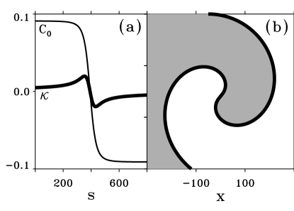
FIG. 2.: A front solution to the kinematic equations (1)-(4). (a) The order parameter $C_{0}$ and the curvature $\kappa$ along the arclength $s$. (b) In the $x-y$ plane the front solution corresponds to a rotating spiral wave. The shaded (light) region corresponds to an up (down) state. Parameters: $a_{1}=4$, $a_{0}=0$, $\epsilon=0.01234$, $\delta=1.0.$

A second application of the kinematic equations is the study of spontaneous spiral-wave nucleation. Spiral-wave nucleation, induced by a transverse instability, has been previously observed in direct simulations of (6) [9]. Figs. 3a-d show the time evolution of a solution to the $C_{0}-\kappa$ equations representing a planar front near the NIB bifurcation and beyond the transverse instability boundary. The initial front pertains to an up state invading a down state ($C_{0}>0$). The transverse instability causes a small dent on the front to grow (Fig. 3b). The negative curvature then triggers the nucleation of a region along the arclength where the propagation direction is reversed ($C_{0}<0$) (Fig. 3c). The pair of fronts in the kinematic equations that bound this region correspond to a pair of counter-rotating spiral waves in the FitzHugh-Nagumo equations (Fig. 3d). With this approach, the two-dimensional spiral-wave nucleation problem is reduced to the considerably simpler problem of domain, or droplet, nucleation in one dimension [20].

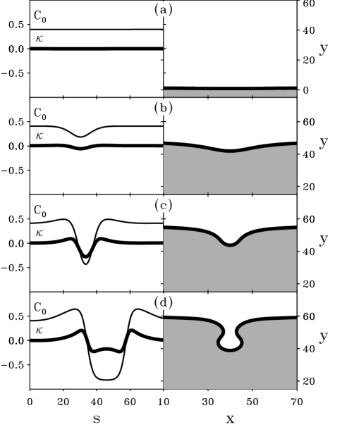
FIG. 3.: Nucleation of a spiral-wave pair in the kinematic equations (1)-(4) Left column: the $C_{0}(s)$ and $\kappa(s)$ profiles. Right column: the front line shape in the $x-y$ plane. Parameters: $a_{1}=4$, $a_{0}=-0.0001$, $\epsilon=0.0115$, $\delta=1.063.$ (a)-(d) are at $t=0,116,136,142$.

We have derived kinematic equations for front motion in two-dimensional bistable systems near a NIB bifurcation. The equations generalize earlier derivations and capture both the core structure of spiral waves and the dynamic process of spiral-wave nucleation. Further investigation is needed to determine if other features of spiral waves, like the meander instability [21], are captured by the equations. Note that front interaction effects are excluded by the choice of the boundary conditions, $v(\mp\infty,s,t)=v_{\pm}$, in Eqs. (17). Such interactions are not significant for the initial stages of spiral wave nucleation or for the symmetric (or nearly symmetric) low curvature spirals studied in this Letter. Front interactions, however, do become significant when highly curved spirals develop, and might play an essential role in the meander instability. Goldstein et al. [22] have recently studied front interactions in the fast inhibitor limit ($\epsilon\gg 1$) where stationary patterns prevail. A combination of the approaches used in these two complementary studies may prove useful in establishing a theory of spiral waves of wider validity.

REFERENCES

[1]Email: aric@lanl.gov
[2]Email: ehud@bgumail.bgu.ac.il
[3]
V. S. Zykov, Simulation of Wave Processes in Excitable Media (Manchester
University Press, Manchester, 1987).
[4]
A. S. Mikhailov, Foundation of Synergetics I: Distributed Active Systems
(Springer-Verlag, Berlin, 1990).
[5]
E. Meron and P. Pelcé, Phys Rev. Lett. 60, 1880 (1988).
[6]
E. Meron, Physics Reports 218, 1 (1992).
[7]
V. Pérez-Muñuzuri, C. Souto, M. Gómez-Gesteira, A. P. Muñuzuri,
V. A. Davydov, and V. Pérez-Villar, Physica D 94, 148 (1996);
P. K. Brazhnik, Physica D 94, 205 (1996).
[8]
K. J. Lee, W. D. McCormick, H. L. Swinney, and J. E. Pearson, Nature
369, 215 (1994); K. J. Lee and H. L. Swinney, Phys. Rev. E
51, 1899 (1995).
[9]
A. Hagberg and E. Meron, Phys. Rev. Lett. 72, 2494 (1994).
[10]
A. Hagberg and E. Meron, Chaos 4, 477 (1994).
[11]
C. Elphick, A. Hagberg, and E. Meron, Phys. Rev. E 51, 3052 (1995).
[12]
P. Coullet, J. Lega, B. Houchmanzadeh, and J. Lajzerowicz, Phys. Rev. Lett.
65, 1352 (1990).
[13]
H. Ikeda, M. Mimura, and Y. Nishiura, Nonl. Anal. TMA 13, 507 (1989).
[14] A. Hagberg and E. Meron, Nonlinearity 7, 805 (1994).
[15]
M. Bode, A. Reuter, R. Schmeling, and H.-G. Purwins, Phys. Lett. A 185,
70 (1994).
[16]
G. Haas, M. Bär, I. G. Kevrekidis, P. B. Rasmussen, H.-H. Rotermund, and
G.Ertl, Phys Rev. Lett. 75, 3560 (1995);
D. Haim, G. Li, Q. Ouyang, W. D. McCormick, H. L. Swinney, A. Hagberg, and E.
Meron, Phys. Rev. Lett. 77, 190 (1996).
[17]
S. Nasuno, N. Yoshimo, and S. Kai, Phys. Rev. E 51, 1598 (1995);
T. Frisch, S. Rica, P. Coullet, and J. M. Gilli, Phys. Rev. Lett. 72,
1471 (1994);
[18]
J. P. Keener, SIAM J. Appl. Math 39, 528 (1980).
[19] A. Hagberg, E. Meron, I. Rubinstein, and B. Zaltzman,
Phys. Rev. Lett. 76, 427 (1996).
[20]
P. C. Fife, Mathematical Aspects of Reacting and Diffusing Systems,
Vol. 28 of Lecture Notes in Biomathematics (Springer-Verlag, New York,
1979).
[21]
A. T. Winfree, Chaos 1, 303 (1991); D. Barkley, Phys. Rev. Lett. 72, 164 (1994).
[22]
R. E. Goldstein, D. J. Muraki, and D. M. Petrich, Phys. Rev. E 53, 3933
(1996).