[

FERMILAB–Pub–96/406-A

patt-sol/9611001 at xyz.lanl.gov

Vortex Dynamics in Dissipative Systems

Abstract

We derive the exact equation of motion for a vortex in two- and three-dimensional non-relativistic systems governed by the Ginzburg-Landau equation with complex coefficients. The velocity is given in terms of local gradients of the magnitude and phase of the complex field and is exact also for arbitrarily small inter-vortex distances. The results for vortices in a superfluid or a superconductor are recovered.

] Vortices are found in a variety of physical systems. Accordingly, the study of these intriguing collective excitations attracts widespread attention among the physics community. Examples of vortices often studied are hydrodynamic vortices, vortices in superfluids, in superconductors and in nematic crystals, and cosmic strings [1, 2]. An important goal is to clarify the mechanisms by which vortices are created and the details of their motion subject to local interactions, such as crossing, merging and intercommutation, as well as long-range forces. These issues have recently been addressed in the context of relativistic scalar field theories [3, 4].

In this Letter we present an analytic derivation of the exact equation of motion for a vortex in a non-relativistic dissipative system. The system we study is one modelled by the extensively studied [5, 6, 7, 8, 9] Ginzburg–Landau equation with complex coefficients (CGL)

$${\textstyle\frac{d}{dt}}\,A=P(A,A^{\ast})A+b\nabla^{2}A$$ (1)

where $A=|A|\exp(iS)$ is a complex field, the function $P$ is given by $P(A,A^{\ast})=\mu-a|A|^{2}$, and $a,b,\mu\in{\bf C}$. By a suitable rescaling of time, space, and $A$, the number of (real) adjustable parameters in the coefficients of eq. (1) may be brought down to two, as is often done. However, we shall keep eq. (1) unscaled for clarity. We study the equation in two and three spatial dimensions.

The reason for selecting the CGL equation is two-fold. Firstly, it is a relatively simple partial differential equation; yet it exhibits the principal features of more complicated oscillatory systems. A prime example of such systems are reaction-diffusion systems, such as the chemical oscillatory Belousov-Zhabotinsky reaction[10, 11].

Secondly, the CGL equation contains a number of interesting special cases. When $a$, $b$, and $\mu$ are purely imaginary the CGL equation coincides with the non-linear Schrödinger equation. The latter equation describes the quantum dynamics of superfluid ${}^{4}\!$He and is known in that context as the Ginzburg-Pitaevskii-Gross equation (GPG) [12]. Furthermore, by employing the Madelung transformation [13] the non-linear Schrödinger equation also transforms into the hydrodynamic equations for an inviscid fluid (the Euler equations). In both cases $|A|^{2}$ corresponds to the (super)fluid mass density and $\nabla S$ is proportional to the velocity of the (super)fluid. We stress that the GPG case is special because it describes a conservative system and the vortex motion can be derived from a Lagrangian. The CGL equation, on the other hand, describes a dissipative system and one is compelled to pursue a direct derivation of the vortex equation of motion, as we do here.

Equation (1) permits solutions in which $A$ has phase singularities (defects). In two space dimensions these are isolated points around which the phase $S$ changes by multiples of $2\pi$. At the same points the magnitude $|A|$ vanishes, so that the complex field $A$ remains single valued, see figure 1.

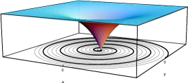
FIG. 1.: One-armed spiral vortex of the CGL field $A=|A|e^{iS}$ in a two-dimensional system. The height of the surface depicts the magnitude $|A|$. The spiraling curves are contour lines of the phase $S$ (isophase lines). The phase change between two thin lines is $\pi/2$.

In the vicinity of a defect the phase is of the form $S=\psi(r)+n(\varphi-\omega t)$ in polar coordinates ($r,\varphi$) [14]. For a constant phase $S$ this is the equation for $|n|$-armed spirals rotating at an angular frequency $\omega$. In three dimensions the defects become one-dimensional strings, or filaments, and the spirals generalize to scroll waves [11, 15] which look like sheets wound around a filament. The filaments may be closed or open (in which case they end on the system boundary) and of arbitrary shape. We shall call a solution with one defect or filament (in two or three dimensions) a spiral vortex, in analogy with the (non-spiral, $\psi^{\prime}(r)=0$) vortex solution of the GPG equation, which describes the circulation of the superfluid around strings of normal-phase fluid. The integer $n$ is the winding number of the vortex and is a topologically conserved quantity in two dimensions but not in three. The core of the vortex is the region where the magnitude $|A|$ deviates significantly from its asymptotic value, see figure 1.

The evolution of a system with (spiral) vortices may be described in terms of the motion of the defects, or filaments, along with values of the fields $|A|$ and $S$ at positions away from the defects or filaments. Such a separation into collective coordinates and field variables is non-trivial, and the present work comprises the first exact treatment of this kind for a dissipative system. The motion of a vortex is affected by modifications in the field $A$ due to the presence of other vortices or system boundaries. If the vortices are assumed to form a dilute system, i.e.  one where the defects are well separated, the influence of variations in the magnitude $|A|$ of the complex field may be neglected, since $|A|$ will assume its asymptotic value at distances much smaller than the inter-defect distance [16]. Under this assumption, the interaction between vortices can be described entirely by the phase $S$. In this approximation Rica and Tirapegui [8] (and in a slightly different form also Ref. [9]) have derived the equation of motion in two space dimensions for the position of the $k$th defect $\mbox{\boldmath$X$}_{k}(t)$ in terms of the portion of the phase $S$ due to other defects, $\theta^{(k)}(\mbox{\boldmath$x$})\equiv S-n_{k}\varphi_{k}$, where $\tan\varphi_{k}=(y-Y_{k})/(x-X_{k})$. Their result (for $|n_{k}|=1$ and $b_{\scriptscriptstyle R}=1$, but here generalized to any value of $n_{k}$ and $b_{\scriptscriptstyle R}$) is

$$\dot{\mbox{\boldmath$X$}}_{k}\equiv{{d\mbox{\boldmath$X$}_{k}}\over{dt}}=2b_{\scriptscriptstyle I}\nabla\theta^{(k)}-2b_{\scriptscriptstyle R}\frac{n_{k}}{|n_{k}|}\hat{\mbox{\boldmath$z$}}\times\nabla\theta^{(k)}{\hskip 4.26773pt{\rm,}}$$ (2)

where $b_{\scriptscriptstyle R}\equiv{\rm Re}\,b$, $b_{\scriptscriptstyle I}\equiv{\rm Im}\,b$, and $\hat{\mbox{\boldmath$z$}}=\hat{\mbox{\boldmath$x$}}\times\hat{\mbox{\boldmath$y$}}$ is normal to the plane. The first term, proportional to the gradient, is that found by Fetter [17] in the GPG limit corresponding to $b_{\scriptscriptstyle R}=0$, $b_{\scriptscriptstyle I}=\hbar/(2m)$ and states that the vortex moves with the local superfluid velocity. The second term is the perpendicular Peach-Koehler term [18] first found in this context by Kawasaki [19].

When the system of spiral vortices cannot be approximated by a dilute system the expression (2) for the defect velocity is no longer valid but will acquire additional terms. We shall take a completely general approach in which the amplitude $|A|$ is allowed to vary. This will enable us to determine the exact motion of a defect also when another defect is located an arbitrarily small distance away, i.e. even when the vortex cores overlap. It will also provide the exact motion of a defect which is arbitrarily near a system boundary. For filaments in a three-dimensional system our treatment will furthermore correctly incorporate interactions with other segments of the same filament.

The corresponding problem for a relativistic scalar field theory was solved by Ben-Ya’acov [4]. His derivation was based strictly on a covariant world-sheet formalism that cannot be applied to a non-relativistic theory. For the CGL equation one must therefore resort to other methods.

Let us consider the general motion of vortices in three space dimensions. The motion in a two-dimensional system can be found from the three-dimensional problem as the special case of straight, aligned vortices.

We may generalize eq. (1) by admitting any continuous function $P(A,A^{\ast})$. The details of $P$ do not enter the derivation. The field $A$ is zero on a collection of one-dimensional strings which are the filaments. Let the position of the filament $\Gamma$ of a vortex be given at time $t$ by $\mbox{\boldmath$X$}(s,t)$, where $s$ is the arclength coordinate along $\Gamma$. We define a local coordinate system along the string as follows [20]. At each point along the string the unit tangent vector $\mbox{\boldmath$T$}=\partial\mbox{\boldmath$X$}/\partial s$, the unit normal vector $N$, and the binormal vector $\mbox{\boldmath$B$}=\mbox{\boldmath$T$}\times\mbox{\boldmath$N$}$ form an orthonormal frame so that any position $x$ in a neighborhood of the string can be expressed as $\mbox{\boldmath$x$}=\mbox{\boldmath$X$}(s,t)+x\mbox{\boldmath$N$}(s,t)+y\mbox{\boldmath$B$}(s,t)$. The coordinate representation $(s,x,y)$ is unique for $x<1/\kappa$ but becomes singular when $x$ reaches or exceeds the radius of curvature $1/\kappa$.

Along the string, the transport of the unit vectors is given by the Frenet-Serret equations [20]

$$\frac{\partial\mbox{\boldmath$T$}}{\partial s}=\kappa\mbox{\boldmath$N$}{{\rm,}\hskip 5.69046pt}\frac{\partial\mbox{\boldmath$N$}}{\partial s}=-\kappa\mbox{\boldmath$T$}+\tau\mbox{\boldmath$B$}{{\rm,}\hskip 5.69046pt}\frac{\partial\mbox{\boldmath$B$}}{\partial s}=-\tau\mbox{\boldmath$N$}{{\rm,}}$$ (3)

where $\kappa$ is the curvature and $\tau$ is the torsion of the string. Let us further introduce the local polar coordinates $r$, $\varphi$ defined by $x=r\cos\varphi$, $y=r\sin\varphi$. In terms of these coordinates, the gradient and Laplacian take the forms

$$\nabla = \mbox{\boldmath$T$}H+\hat{\mbox{\boldmath$r$}}\frac{\partial\,}{\partial r}+\hat{\mbox{\boldmath$\varphi$}}\frac{1}{r}\frac{\partial\,}{\partial\varphi}$$ (4)

$$\nabla^{2} = H^{2}+\frac{\partial^{2}\,}{\partial r^{2}}+\frac{1}{r}\frac{\partial\,}{\partial r}+\frac{1}{r^{2}}\frac{\partial^{2}\,}{\partial\varphi^{2}}$$ (6)

$$\mbox{}-\frac{\kappa}{1-\kappa r\cos\varphi}\left(\cos\varphi\frac{\partial\,}{\partial r}-\sin\varphi\frac{1}{r}\frac{\partial\,}{\partial\varphi}\right)\,,$$

where

$$H=\frac{1}{1-\kappa r\cos\varphi}\left(\frac{\partial\,}{\partial s}-\tau\frac{\partial\,}{\partial\varphi}\right)\,.$$ (7)

We now proceed to find the velocity $\dot{\mbox{\boldmath$X$}}(s,t)$ of the filament $\Gamma$. Because this string of zeros of the function $A$ has no transverse extension and is a feature of a solution of an underlying local field theory, its motion should be determined from the behavior of the fields $|A|$ and $S$ in an infinitesimal neighborhood of the filament. It will be sufficient to study the fields within a distance $\varepsilon\ll\min(d,1/\kappa)$, where $d$ is the shortest distance to another string segment [21]. This condition ensures uniqueness of the coordinate representation.

The phase field $S$ is multi-valued and satisfies $S(s,r,\varphi+2\pi;t)-S(s,r,\varphi;t)=n\,2\pi$ for $0<r<\varepsilon$. Let us therefore split $S=\chi+\theta$ in such a way that $\chi$ contains all multi-valued contributions to the phase and depends on time only through the position of the filament $\Gamma$. For a straight (or two-dimensional) isolated vortex one may choose $\chi=n\varphi$. A consistent description of the multi-valued phase of an arbitrarily shaped vortex filament requires, however, a global realization such as the Biot-Savart integral,

$$\nabla\chi=\frac{n}{2}\int_{\Gamma}d\mbox{\boldmath$X$}\times\frac{\mbox{\boldmath$x$}-\mbox{\boldmath$X$}}{|\mbox{\boldmath$x$}-\mbox{\boldmath$X$}|^{3}}{\hskip 4.26773pt{\rm.}}$$ (8)

This expression is known to contain logarithmic divergencies as $r\to 0$, as well as functions of the azimuthal angle $\varphi$ that are multi-valued at $r=0$ [2]. We therefore absorb in $\chi$ any part of $S$ that is non-differentiable at $r=0$. Similarly, we may write $|A|=Rw$, where $\ln R$ depends on the filament position and contains all contributions to $\ln|A|$ that are non-differentiable at $r=0$. For a straight isolated vortex one may choose $R=r^{|n|}$. Thus $\theta$ and $\ln w$ are differentiable and it follows that the time derivatives $\dot{\theta}$ and $\dot{w}$ are finite for $r<\varepsilon$. We remark that the choice of $\chi$ and $R$ is not unique, since $S$ and $|A|$ are invariant under two independent local symmetries

$$\chi\to\chi+\delta,~{}\theta\to\theta-\delta\quad;\quad R\to Rf,~{}w\to wf^{-1}{\hskip 4.26773pt{\rm,}}$$ (9)

where $\delta$ and $\ln f$ are differentiable.

With these definitions the real and imaginary parts of equation (1) lead to the two equations

$${\textstyle\frac{d}{dt}}\ (\ln R+\ln w) = {\rm Re}(P)+b_{\scriptscriptstyle R}Q_{1}-b_{\scriptscriptstyle I}Q_{2}{\hskip 4.26773pt{\rm,}}$$ (10)

$${\textstyle\frac{d}{dt}}\ (\theta+\chi) = {\rm Im}(P)+b_{\scriptscriptstyle I}Q_{1}+b_{\scriptscriptstyle R}Q_{2}{\hskip 4.26773pt{\rm,}}$$ (11)

where

$$Q_{1} = \nabla^{2}\ln R+\nabla^{2}\ln w$$ (13)

$$\mbox{}+(\nabla\ln R+\nabla\ln w)^{2}-(\nabla\chi+\nabla\theta)^{2}{\hskip 4.26773pt{\rm,}}$$

$$Q_{2} = \nabla^{2}\chi+\nabla^{2}\theta+2(\nabla\ln R+\nabla\ln w)\cdot(\nabla\chi+\nabla\theta).$$ (14)

The time derivative $d/dt$ in eqs. (10) and (11), which is to be evaluated in the lab frame, is related to the time derivative $\partial/\partial t$ in the moving reference frame of the local segment of the filament by $d/dt=-\dot{\mbox{\boldmath$X$}}\cdot\nabla+\partial/\partial t$.

In order to include logarithmic divergencies as well as multi-valuedness as $r\to 0$, we write $\nabla\chi=f_{1}\hat{\mbox{\boldmath$r$}}+(n/r+f_{2})\hat{\mbox{\boldmath$\varphi$}}+\lambda_{1}\mbox{\boldmath$T$}$ and $\nabla\ln R=(|n|/r+f_{3})\hat{\mbox{\boldmath$r$}}+f_{4}\hat{\mbox{\boldmath$\varphi$}}+\lambda_{2}\mbox{\boldmath$T$}$, where

$$f_{i}(r,\varphi,s,t)=g_{i}(\varphi,s,t)+h_{i}(\varphi,s,t)\ln{\kappa r}+{\cal O}(r)$$ (15)

and ${\cal O}(r)$ denotes any terms that vanish as $r\to 0$. It can be easily confirmed from this equation (as well as argued on general grounds) that $\partial\chi/\partial t$, $\partial\chi/\partial s$, $\partial(\ln R)/\partial t$, $\partial(\ln R)/\partial s$, $\lambda_{1}$ and $\lambda_{2}$ have well-defined finite limits as $r\to 0$. We require that $\nabla\chi$ and $\nabla\ln R$ be integrable, and that they satisfy the following condition near the filament:

$$\nabla\chi-\frac{n}{|n|}\mbox{\boldmath$T$}\times\nabla\ln R=\mbox{\boldmath$C$}(s,t)+{\cal O}(r){\hskip 4.26773pt{\rm.}}$$ (16)

The arbitrary vector $C$ corresponds to a choice of gauge in eq. (9). In the symmetric gauge $R=r^{|n|}$, $\chi=n\varphi$ for a straight (or two-dimensional) isolated vortex we have $\mbox{\boldmath$C$}={\bf 0}$.

Since $\theta$ and $\ln w$ are differentiable, the singularities of $\nabla\chi$ and $\nabla\ln R$ at $r=0$ must satisfy eqs. (10) and (11) order by order. This last condition together with eq. (16), leads to the coupled non-linear system

$$\nabla\ln R\cdot\mbox{\boldmath$u$}+b_{\scriptscriptstyle R}q_{1}-b_{\scriptscriptstyle I}q_{2} = {\rm regular}$$ (17)

$$\nabla\chi\cdot\mbox{\boldmath$u$}+b_{\scriptscriptstyle I}q_{1}+b_{\scriptscriptstyle R}q_{2} = {\rm regular}{\hskip 4.26773pt{\rm,}}$$ (18)

where $q_{1}=\nabla^{2}\ln R+(\nabla\ln R)^{2}-(\nabla\chi)^{2}$, $q_{2}=\nabla^{2}\chi+2\nabla\ln R\cdot\nabla\chi$ and $\mbox{\boldmath$u$}=\dot{\mbox{\boldmath$X$}}+2b_{\scriptscriptstyle R}(\nabla\ln w+\frac{n}{|n|}\mbox{\boldmath$T$}\times\nabla\theta)-2b_{\scriptscriptstyle I}(\nabla\theta-\frac{n}{|n|}\mbox{\boldmath$T$}\times\nabla\ln w)$.

Cancellation of terms of order $r^{-1}$ in eq. (17) leads to two equations for the perpendicular components of $u$. The integrability condition provides four first-order differential equations relating the functions $g_{i}$ and $h_{i}$, and together with four algebraic relations resulting from eq. (16) the system can be solved in terms of four constants of integration. The perpendicular components of $u$ are then uniquely determined in terms of $C$. Furthermore, the singular terms of order $r^{-1}\ln\kappa r$ in eq. (17) cancel. It is always possible to set the tangential velocity, which is void of physical meaning, to zero by a time-dependent reparametrization $s\to s(t)$. In the language of relativistic string theory, this is referred to as world-sheet reparametrization invariance. The exact result for the velocity of the vortex filament is

$${\dot{\mbox{\boldmath$X$}}} = {b_{\scriptscriptstyle I}\left(\kappa{{n}\over{|n|}}\mbox{\boldmath$B$}+2(\nabla_{\perp}{\theta}+\mbox{\boldmath$C_{\perp}$})-2{{n}\over{|n|}}\mbox{\boldmath$T$}\times\nabla\ln{w}\right)}$$ (19)

$$+ {b_{\scriptscriptstyle R}\left(\kappa\mbox{\boldmath$N$}-2\nabla_{\perp}\ln w-2\frac{n}{|n|}\mbox{\boldmath$T$}\times(\nabla\theta+\mbox{\boldmath$C$})\right)}{\hskip 4.26773pt{\rm,}}$$ (20)

where $(~{})_{\perp}=-\mbox{\boldmath$T$}\times[\mbox{\boldmath$T$}\times(~{})]$ and the fields on the right-hand side are to be evaluated at the filament position $\mbox{\boldmath$X$}(s,t)$. The exact two-dimensional result is obtained as $\kappa\to 0$.

The value of $\dot{\mbox{\boldmath$X$}}$ is independent of the choice of gauge for $R$ and $\chi$. Indeed, substituting $C$ from eq. (16) into eq. (19) we obtain the manifestly invariant expression

$${\dot{\mbox{\boldmath$X$}}} = \lim_{r\to 0}\left[{b_{\scriptscriptstyle I}\!\!\left(\kappa{{n}\over{|n|}}\mbox{\boldmath$B$}+2\nabla_{\perp}S-2{{n}\over{|n|}}\mbox{\boldmath$T$}\times\nabla\ln|A|\right)}\right.$$ (22)

$$~{}~{}~{}~{}~{}~{}+\left.{b_{\scriptscriptstyle R}\!\!\left(\kappa\mbox{\boldmath$N$}-2\nabla_{\perp}\ln|A|-2{{n}\over{|n|}}\mbox{\boldmath$T$}\times\nabla S\right)}\right].{}$$

in which the filament velocity is written in terms of gradients of the magnitude and phase of the original complex field $A$. Let us define the complex velocity $\dot{Z}\equiv(\mbox{\boldmath$N$}+i\mbox{\boldmath$B$})\cdot\dot{\mbox{\boldmath$X$}}$ and express the derivatives in eq. (22) in terms of $z\equiv x+iy$ and its conjugate $z^{\ast}$. Then a quite beautiful result emerges:

$$\left\{\begin{array}[]{ll}\dot{Z}=b\left(-4\frac{\partial~{}}{\partial z^{\ast}}\ln A(z,z^{\ast})+\kappa\right)&,\ n\geq 1\\[8.61108pt] \dot{Z}{}^{\ast}=b\left(-4\frac{\partial~{}}{\partial z}\ln A(z,z^{\ast})+\kappa\right)&,\ n\leq-1{\hskip 4.26773pt{\rm,}}\end{array}\right.$$ (23)

where the right-hand side is to be evaluated at $z\!=\!z^{\ast}\!=\!0$.

The results are to be interpreted as follows: The velocity of the central filament of a vortex gets contributions from the curvature $\kappa$ of the filament and from local gradients of the magnitude $|A|$ and phase $S$ of the complex field. A cylindrically symmetric solution $A=\rho(r)\exp[i(\psi(r)+n(\varphi-\omega t))]$, for which $\rho=|A|\sim r^{|n|}$ and $\psi^{\prime}(0)=0$, contributes nothing to the velocity and corresponds to a straight (or two-dimensional) isolated vortex at rest with respect to the lab frame. Non-zero gradient contributions appear as a result of deviations from cylindrical symmetry in $|A|$ and $S$. In a symmetric gauge with $\mbox{\boldmath$C$}={\bf 0}$, these deviations are represented by $w$ and $\theta$. The asymmetries arise from the presence of other vortices, system boundaries, or (in three dimensions) other segments of the same filament, causing the vortex to move.

In the $\mbox{\boldmath$C$}={\bf 0}$ gauge the expression (19) reproduces a variety of results obtained previously for special cases. For $\kappa=0$ and $\nabla\ln w\approx 0$ it reduces to eq. (2) corresponding to a two-dimensional dilute system [8]. In the GPG limit $b_{\scriptscriptstyle R}=0$ the expression (19) coincides with that derived by Lee [22], who used a different method to find the velocity. For $b_{\scriptscriptstyle I}=0$, eq. (1) describes the non-linear diffusion of two fluid components with identical diffusion constants. In this limit the contribution to ${\dot{\mbox{\boldmath$X$}}}$ from curvature, $b_{\scriptscriptstyle R}\kappa\mbox{\boldmath$N$}$, agrees with the result of Ref. [15].

The expressions (19)–(23) for the velocity are exact also for an arbitrarily small distance between filaments. This makes the formulation well suited for theoretical or numerical investigations of local vortex interactions, such as crossing, merging and intercommutation, in which the vortex cores overlap [3, 23]. We caution that the GPG equation does not provide a realistic model for the core of a superfluid vortex, since there the core width is comparable to interatomic distances. For magnetic flux vortices in a superconductor, however, the core width is much larger and a classical description is justified. Such vortices are solutions of eq. (1) with the substitution $\nabla\to\nabla+2ie\mbox{\boldmath$A$}/(\hbar c)$, where $A$ is the vector potential and $2e$ is the charge of a Cooper pair. The corresponding filament velocity is easily obtained by adding $2e\mbox{\boldmath$A$}/(\hbar c)$ to $\nabla\theta$ in eq. (19) or to $\nabla S$ in eq. (22) [22].

In summary, we have derived the exact equation of motion for a vortex in a large class of models of a non-relativistic complex field described by the complex Ginzburg–Landau equation (1) with an arbitrary, continuous function $P(A,A^{\ast})$. The velocity is expressed in terms of local gradients of the magnitude and phase of the complex field $A$. The result agrees with that of Ref. [8] (our eq. 2) in the case of a dilute two-dimensional system of vortices, but for the general non-dilute case in two and three dimensions we find additional contributions to the velocity corresponding to the asymmetry of the magnitude $|A|$ around the vortex.

We are grateful to E. Copeland for crucial remarks relating to the three-dimensional case and to T. Bohr for useful discussions and for pointing us in the direction of Ref. [8]. Support for O.T. was provided by DOE and NASA under Grant NAG5-2788 and by the Swedish Natural Science Research Council (NFR), for E.S. by the Danish Natural Science Research Council.

REFERENCES

- [1] D.R. Tilley and J. Tilley, Superfluidity and Superconductivity, 2nd edition (Hilger, 1986); P.G. deGennes, The Physics of Liquid Crystals (Clarendon, Oxford, 1974); A. Vilenkin and E.P.S. Shellard, Cosmic strings and other topological defects (Cambridge Univ. Press, 1994).
- [2] G. K. Batchelor, An Introduction to Fluid Dynamics (Cambridge University Press, 1970).
- [3] U. Ben-Ya’acov, Phys. Rev. D 52, 1065 (1995) .
- [4] U. Ben-Ya’acov, Nucl. Phys. B382, 597 (1992).
- [5] M. C. Cross and P. C. Hohenberg, Rev. Mod. Phys. 65, 851 (1993).
- [6] Y. Kuramoto Chemical Oscillations, Waves, and Turbulence (Springer-Verlag, Berlin, 1984).
- [7] P. Coullet, L. Gil, and J. Lega, Phys. Rev. Lett. 62, 1619 (1989); L. Gil, J. Lega, and J. L. Meunier, Phys. Rev. A 41, 1138 (1990); T. Bohr, A. W. Pedersen, and M. H. Jensen, Phys. Rev. A 42, 3626 (1990); I. S. Aranson, L. Aranson, L. Kramer, and A. Weber, Phys. Rev. A 46, R2992 (1992); G. Huber, P. Alstrøm and T. Bohr, Phys. Rev. Lett. 69, 2480 (1992).
- [8] S. Rica and E. Tirapegui, Physica D 48, 396 (1991) .
- [9] C. Elphick and E. Meron, Physica D 53, 385 (1991).
- [10] See e.g. S. Müller, T. Plesser, and B. Hess, Physica D 24, 71 (1987).
- [11] A. T. Winfree and S. H. Strogatz, Physica D 8, 35 (1983).
- [12] V. T. Ginzburg and P. Pitaevskii, Zh. Eksp. Teor. Fiz. 34, 1240 (1958) [Sov. Phys. JETP 7, 858 (1958)]; E. P. Gross, Nuovo Cimento 20, 454 (1961).
- [13] E. Madelung, Z. Phys. 40, 322 (1927).
- [14] P. S. Hagan, SIAM J. Appl. Math. 42, 762 (1982).
- [15] J. P. Keener, Physica D 31, 269 (1988); J. P. Keener and J. J. Tyson, Physica D 44, 191 (1990).
- [16] In the GPG equation this corresponds to the incompressible approximation.
- [17] A. L. Fetter, Phys. Rev. 151, 100 (1966).
- [18] M. Peach and J. S. Koehler, Phys. Rev. 80, 436 (1950).
- [19] K. Kawasaki, Prog. Theor. Phys. Suppl. 79, 161 (1984).
- [20] See e.g. M. Spivak, A Comprehensive Introduction to Differential Geometry, 2nd edition, Volume II, Chapter 1 (Publish or Perish, Wilmington, Delaware, 1979).
- [21] The shortest distance from a fixed string segment at on the th vortex to another string segment at is defined as the smallest non-zero value of , as and are varied, that corresponds to a local minimum with respect to .
- [22] K. Y. Lee, Vortices and sound waves in superfluids, CU-TP-652, NI-94-013, cond-mat/9409046.
- [23] J. Dziarmaga, Dynamics of overlapping vortices in complex scalar fields, cond-mat/9503068, to appear in Acta Phys. Pol (September, 1996).