Origin of Relativistic Effects in the Reaction D(e,e’p)n at GeV Energies

Abstract

In a series of recent publications, a new approach to the non-relativistic reduction of the electromagnetic current operator in calculations of electro-nuclear reactions has been introduced. In one of these papers [1], the conjecture that at energies of a few GeV, the bulk of the relativistic effects comes from the current and not from the nuclear dynamics was made, based on the large relativistic effects in the transverse-longitudinal response. Here, we explicitly compare a fully relativistic, manifestly covariant calculation performed with the Gross equation, with a calculation that uses a non-relativistic wave function and a fully relativistic current operator. We find very good agreement up to missing momenta of $400$ MeV/c, thus confirming the previous conjecture. We discuss slight deviations in cross sections for higher missing momenta and their possible origin, namely p-wave contributions and off-shell effects.

I Introduction

Currently, there is a lot of activity in the field of electron scattering from nuclei at a few GeV. There exists a broad experimental program of electron scattering studies at Jefferson Lab, MAMI, and Bates, aimed at understanding the short range structure of nuclei and the properties of nucleons in the nuclear medium. It would be ideal to perform theoretical calculations of these processes in a completely microscopic fashion, starting from a Lagrangian. Such an approach would contain explicit relativistic treatments of the nuclear dynamics and the electromagnetic current, as well as a consistent treatment of the initial nuclear state and the in general quite complicated hadronic final state. In practice, for high-energy inelastic electron scattering, it is very difficult to calculate both the nuclear ground state and the final hadronic scattering state consistently and it is unlikely that a consistent, fully microscopic and, therefore, relativistic treatment will be available for medium and heavier nuclei in the near future. Currently, there are several approximate calculations for particular electro-nuclear reactions available for few-body systems [2, 3]. However, it is difficult to extend these approaches for the few-body systems to energies above the pion emission threshold. With the considerable effort one expects will be put into this field, in the next few years calculations for the few GeV regime for reactions with deuteron targets will hopefully become available. For heavy nuclei, there are only relativistic mean-field calculations available, which do not allow for the investigation of ground-state correlations.

Therefore, it is an essential question if the main physical features of high energy electro-nuclear reactions can be incorporated in theoretical calculations in an effective manner, which would allow one to perform these calculations for a variety of target nuclei in the few GeV regime. One essential feature at GeV energies is relativity, and this is the topic with which we concern ourselves in this paper.

Relativistic effects show up in three places: in the kinematics, in the electromagnetic current, and in the nuclear/hadronic dynamics. The first point, relativistic kinematics, is trivial. In order to treat the nuclear dynamics in a relativistic way, one can solve the Bethe Salpeter equation or one of its variations, e.g. the Gross equation [9]. The electromagnetic current has traditionally been used in a non-relativistic reduction, which assumes that the transferred momentum, transferred energy and initial nucleon momentum are small compared to the nucleon mass. These assumptions are not valid for modern day experiments with GeV electron beams and energy and momentum transfers of 1 GeV or more, and there exist several improved schemes. In a series of recent publications [1, 4, 5, 6] a new approach to the problem of the non-relativistic reduction of the current was introduced, and in [1], it was conjectured that the bulk of the relativistic effects at energies of a few GeV stem from the current, not from the nuclear dynamics. This conjecture is based on the large enhancement of the transverse-longitudinal response observed in this scheme, which was also seen in the fully relativistic calculation of [3]. If this conjecture is indeed true, relativity could be taken into account by applying the operator introduced in [1, 4, 5, 6] together with non-relativistic wave functions to the calculation of electro-nuclear reactions. This would obviously be very useful.

Although strong evidence was presented in [1], this conjecture can only be confirmed by a direct comparison to a fully relativistic, microscopic calculation. This comparison is carried out in the following sections for the deuteron target. As we wish to concentrate for the moment on the problem of relativity only, we perform this comparison for Plane Wave Impulse Approximation (PWIA). A realistic calculation must treat final state interactions, too, but the conjecture can be tested successfully at the plane wave level. Moreover, a fully microscopic, consistent calculation of final state interaction at GeV energies is extremely difficult and not available at the moment. The high energy final state interactions are usually treated within the framework of Glauber theory [7].

II Brief review of formalism and notation

We start by introducing some notation and giving a brief summary of the basic formalism of $(e,e^{\prime}p)$ reactions. More details can be found in [8, 10].

The differential cross section in the lab frame is

$$\left(\frac{d\sigma^{5}}{d\epsilon^{\prime}d\Omega_{e}d\Omega_{N}}\right)_{fi}^{h} = \frac{m_{N}\,m_{f}\,p_{N}}{8\pi^{3}\,m_{i}}\,\sigma_{Mott}\,f_{rec}^{-1}\,$$ (3)

$$\Big{[}\left(v_{L}R_{fi}^{L}+v_{T}R^{T}_{fi}+v_{TT}R_{fi}^{TT}+v_{TL}R_{fi}^{TL}\right)$$

$$+h\left(v_{T^{\prime}}R_{fi}^{T^{\prime}}+v_{TL^{\prime}}R_{fi}^{TL^{\prime}}\right)\Big{]}\,,$$

where $m_{i}$, $m_{N}$ and $m_{f}$ are the masses of the target nucleus, the ejectile nucleon and the residual system, $p_{N}$ and $\Omega_{N}$ are the momentum and solid angle of the ejectile, $\epsilon^{\prime}$ is the energy of the detected electron and $\Omega_{e}$ is its solid angle. The helicity of the electron is denoted by $h$. The Mott cross section is

$$\sigma_{Mott}=\left(\frac{\alpha\cos(\theta_{e}/2)}{2\varepsilon\sin^{2}(\theta_{e}/2)}\right)^{2}$$ (4)

and the recoil factor is given by

$$f_{rec}=|1+\frac{\omega p_{x}-E_{x}q\cos\theta_{x}}{m_{i}\,p_{x}}|\,.$$ (5)

The coefficients $v_{K}$ are the leptonic coefficients, and the $R_{K}$ are the response functions which are defined by

$$R_{fi}^{L} \equiv |\rho(\vec{q})_{fi}|^{2}$$ (6)

$$R_{fi}^{T} \equiv |J_{+}(\vec{q})_{fi}|^{2}+|J_{-}(\vec{q})_{fi}|^{2}$$ (7)

$$R_{fi}^{TT} \equiv 2\,\Re\,\big{[}J_{+}^{*}(\vec{q})_{fi}\,J_{-}(\vec{q})_{fi}\big{]}$$ (8)

$$R_{fi}^{TL} \equiv -2\,\Re\,\big{[}\rho^{*}(\vec{q})_{fi}\,(J_{+}(\vec{q})_{fi}-J_{-}(\vec{q})_{fi})\big{]}$$ (9)

$$R_{fi}^{T^{\prime}} \equiv |J_{+}(\vec{q})_{fi}|^{2}-|J_{-}(\vec{q})_{fi}|^{2}$$ (10)

$$R_{fi}^{TL^{\prime}} \equiv -2\,\Re\,\big{[}\rho^{*}(\vec{q})_{fi}\,(J_{+}(\vec{q})_{fi}+J_{-}(\vec{q})_{fi})\big{]}\,,$$ (11)

where the $J_{\pm}$ are the spherical components of the current. For our calculations, we have chosen the following kinematic conditions: the z-axis is parallel to $\vec{q}$, the missing momentum is defined as $\vec{p}_{m}\equiv\vec{q}-\vec{p}_{N}$, so that in Plane Wave Impulse Approximation (PWIA), the missing momentum is equal to the negative initial momentum of the struck nucleon in the nucleus, $\vec{p}_{m}=-\vec{p}$. We denote the angle between $\vec{p}_{m}$ and $\vec{q}$ by $\theta$, and the term “parallel kinematics” indicates $\theta=0^{o}$, “perpendicular kinematics” indicates $\theta=90^{o}$, and “anti-parallel kinematics” indicates $\theta=180^{o}$. Note that both this definition of the missing momentum and the definition with the other sign are used in the literature. In this paper, we assume that the experimental conditions are such that either the kinetic energy of the outgoing nucleon and the angles of the missing momentum, $\theta$, and the azimuthal angle $\phi$, are fixed, or that the transferred energy $\omega$, the transferred momentum $\vec{q}$, and the azimuthal angle $\phi$, are fixed. In the former case, the transferred energy and momentum change for changing missing momentum, in the latter situation, the kinetic energy and polar angle of the outgoing proton change for changing missing momentum.

The electromagnetic current operator

$$J^{\mu}(P\Lambda;P^{\prime}\Lambda^{\prime})=\bar{u}(P^{\prime}\Lambda^{\prime})\left[F_{1}\gamma^{\mu}+\frac{i}{2m_{N}}F_{2}\sigma^{\mu\nu}Q_{\nu}\right]u(P\Lambda)\,$$ (12)

where $P,P^{\prime}$ indicate the four-momenta of the nucleon, can be rewritten in a form that is more suitable for application to nuclear problems:

$$J^{\mu}(P\Lambda;P^{\prime}\Lambda^{\prime})\equiv\chi_{\Lambda^{\prime}}^{\dagger}\,\,\bar{J}^{\mu}(P;P^{\prime})\,\,\chi_{\Lambda}$$ (13)

with

$$\bar{J}^{o} = \rho=f_{o}\left(\xi_{o}+\,i\,\,\xi_{o}^{\prime}\,\left(\vec{q}\times\vec{p}\right)\cdot\vec{\sigma}\right)$$ (14)

$$\bar{J}^{3} = \,\,\frac{\omega}{q}\,\,\bar{J}^{o}$$ (15)

$$\bar{J}^{\bot} = f_{o}\left(\xi_{1}\left[\,\vec{p}-\left(\frac{\vec{q}\cdot\vec{p}}{q^{2}}\right)\vec{q}\,\right]\right.$$ (16)

$$-i \left\{\xi_{1}^{\prime}\left(\vec{q}\times\vec{\sigma}\right)+\left.\xi_{2}^{\prime}\left(\vec{q}\cdot\vec{\sigma}\right)\left(\vec{q}\times\vec{p}\right)+\xi_{3}^{\prime}\left[\left(\vec{q}\times\vec{p}\right)\cdot\vec{\sigma}\right]\left[\vec{p}-\left(\frac{\vec{q}\cdot\vec{p}}{q^{2}}\right)\vec{q}\right]\right\}\right).$$ (17)

Here, $f_{o},\xi_{i},\xi_{i}^{\prime}$ are all functions of $\omega,q,p^{2}$; their explicit forms are given in [1]. For the reasons explained in [1], we refer to the operator associated with $\xi_{o}$ as zeroth-order charge operator, we call the term containing the $\xi_{o}^{\prime}$ first-order spin-orbit operator, the term containing $\xi_{1}$ first-order convection current, the term containing $\xi_{1}^{\prime}$ zeroth-order magnetization current, the term containing $\xi_{2}^{\prime}$ first-order convective spin-orbit term, and the term containing $\xi_{3}^{\prime}$ second-order convective spin-orbit term.

Note that there are more terms in the full current than with the commonly used strict non-relativistic reduction, which assumes that the transferred momentum $q$ is smaller than the nucleon mass, and that both the initial nucleon momentum and the transferred energy are smaller than $q$ and therefore much smaller than the nucleon mass. Under these assumptions, the current operator simplifies to the form

$$\bar{J}^{o}_{nonrel} = G_{E}$$ (18)

$$\bar{J}^{\perp}_{nonrel} = -\frac{i}{2\,m_{N}}\,G_{M}\,\left(\vec{q}\times\vec{\sigma}\right)+\frac{1}{m_{N}}\,G_{E}\,\left(\vec{p}-\frac{\vec{q}\cdot\vec{p}}{q^{2}}\,\vec{q}\right)\,,$$ (19)

which contains only the zeroth-order charge operator, the zeroth-order magnetization current and the first-order convection current.

In non-relativistic Plane Wave Impulse Approximation (PWIA), we have

$$\frac{d^{5}\sigma}{d\epsilon^{\prime}d\Omega_{e}d\Omega_{N}}=\frac{m_{N}\,m_{f}\,p_{N}}{m_{i}}\,\sigma_{eN}\,f_{rec}^{-1}\,n(\vec{p})\,,$$ (20)

where $n(\vec{p})$ is the momentum distribution, and the $eN$ cross section is given by

$$\sigma_{eN}=\sigma_{Mott}\sum_{k}v_{k}R_{k}^{single\,nucleon}$$ (21)

and the single nucleon responses are related to the nuclear responses by

$$R_{K}^{nucleus}=(2\pi)^{3}\,R_{k}^{single\,nucleon}\,n(\vec{p})$$ (22)

so that one has in total:

$$\frac{d^{5}\sigma}{d\epsilon^{\prime}d\Omega_{e}d\Omega_{N}}=\frac{m_{N}\,m_{f}\,p_{N}}{m_{i}}\,f_{rec}^{-1}\,\sigma_{Mott}\,n(\vec{p})\,\sum_{k}v_{k}R_{k}^{single\,nucleon}$$ (23)

The momentum distribution is simply the Fourier transform of the wave function, and in the non-relativistic case takes the form:

$$n(\vec{p})=\frac{1}{2\pi^{2}}(u(p)^{2}+w(p)^{2})$$ (24)

where $u(p),w(p)$ are the S-wave and D-wave functions in momentum space, and the normalization condition is

$$\int d^{3}\vec{p}\,n(\vec{p})=1$$ (25)

Note that the different parts of the wave function do not interfere as long as the target deuteron is unpolarized. The above formulas, and especially the factorization into $eN$ cross section and momentum distribution, is valid only in non-relativistic PWIA, not in PWBA. The Born approximation for $(e,e^{\prime}p)$ scattering contains in addition to the graph where the photon couples to to the proton the graph where the photon couples to the neutron. The difference between PWIA and PWBA for high energy transfers is small, as the second contribution involves the deuteron wave function taken at the momentum of the outgoing proton, which is high, and therefore the value of the deuteron wave function is very small. However, the PWBA is sufficient to break factorization and to permit the interference of the different wave function components. In the following, we present explicit analytic formulas for PWIA; these formulas are considerably simpler than the corresponding PWBA expressions. For consistency, the numerical results are also presented in PWIA. Their deviation from the PWBA results at the kinematics used here is very small, on the order of a few percent. None of our results and conclusions are affected by this.

For the full current operator, the single-nucleon responses take the following form:

$$R_{L}^{sn} = f_{o}^{2}(\xi_{o}^{2}+\kappa^{2}\delta^{2}\xi_{o}^{\prime 2})$$ (26)

$$= \frac{\kappa^{2}}{\tau}(G_{E}^{2}+\delta^{2}W_{2})$$ (27)

$$R_{T}^{sn} = f_{o}^{2}(2\kappa^{2}\xi_{1}^{\prime 2}+\kappa^{4}\delta^{2}\xi_{2}^{\prime 2}+\delta^{2}\xi_{1}^{2}+\kappa^{2}\delta^{4}\xi_{3}^{\prime 2}-2\kappa^{2}\delta^{2}\xi_{1}^{\prime}\xi_{3}^{\prime})$$ (28)

$$= 2W_{1}+\delta^{2}W_{2}$$ (29)

$$R_{TT}^{sn} = f_{o}^{2}(\kappa^{4}\delta^{2}\xi_{2}^{\prime 2}+2\kappa^{2}\delta^{2}\xi_{1}^{\prime}\xi_{3}^{\prime}-\delta^{2}\xi_{1}^{2}-\kappa^{2}\delta^{4}\xi_{3}^{\prime 2})\cos(2\varphi)$$ (30)

$$= -\delta^{2}W_{2}\cos(2\varphi)$$ (31)

$$R_{TL}^{sn} = 2\sqrt{2}\cos(\varphi)f_{o}^{2}(\delta\xi_{o}\xi_{1}+\kappa^{2}\delta\xi_{o}^{\prime}(\xi_{1}^{\prime}-\delta^{2}\xi_{3}^{\prime}))$$ (32)

$$= 2\sqrt{2}\cos(\varphi)\frac{\kappa}{\sqrt{\tau}}\sqrt{1+\tau+\delta^{2}}\delta W_{2}$$ (33)

with the abbreviations $W_{1}\equiv\tau G_{M}^{2}$ and $W_{2}\equiv\frac{1}{1+\tau}(G_{E}^{2}+\tau G_{M}^{2})$.

For the strict non-relativistic reduction, the single nucleon responses are given by:

$$R_{L}^{sn} = G_{E}^{2}$$ (34)

$$R_{T}^{sn} = 2\kappa^{2}\,G_{M}^{2}+\delta^{2}G_{E}^{2}$$ (35)

$$R_{TT}^{sn} = -\delta^{2}G_{E}^{2}\cos(2\varphi)$$ (36)

$$R_{TL}^{sn} = \delta G_{E}^{2}2\sqrt{2}\cos(\varphi)$$ (37)

The dimensionless variables are defined as follows:

$$\kappa = \frac{|\vec{q}|}{2m_{N}}$$ (38)

$$\delta = \frac{p_{\perp}}{m_{N}}$$ (39)

$$\tau = \kappa^{2}-\lambda^{2}$$ (40)

$$\lambda = \frac{\omega}{2m_{N}}$$ (41)

FIG. 1.: This figure shows the relevant kinematic quantities for the electrodisintegration of the deuteron in PWIA.

The above formulas for the non-relativistic PWIA do not hold for a relativistic treatment of the situation. Besides the presence of singlet and triplet P waves, which appear only in a full relativistic treatment of the hadronic state, the factorization breaks down. This fact was observed earlier, e.g. in [11, 12, 13], and can be attributed to the presence of negative energy states in the relativistic treatment. To illustrate this point, we write out the expression for the hadronic tensor $W^{\mu\nu}$ in the $D(e,e^{\prime}p)n$ reaction in the relativistic plane wave impulse approximation (RPWIA). The relevant kinematic quantities are identified in Fig. 1; in the following, $\check{p}$ indicates a four-vector with on-shell energy momentum relation, i.e. $p^{o}=E_{p}:=\sqrt{\vec{p}\,^{2}+m^{2}}$:

$$W^{\mu\nu} = \frac{1}{3}\mbox{Tr}(J^{\mu}(-q)S_{F}(p_{1}+q)J^{\nu}(q)$$ (44)

$$\sum_{\lambda_{d}\lambda_{2}}\sum_{\lambda_{1}^{\prime}\lambda_{1}}[u(\vec{p}_{1},\lambda_{1})\Psi^{+}_{\lambda_{1}\lambda_{2}\lambda_{d}}(\vec{p}_{1})+v(-\vec{p}_{1},\lambda_{1})\Psi^{-}_{\lambda_{2}\lambda_{1}\lambda_{d}}(\vec{p}_{1})]$$

$$[\bar{u}(\vec{p}_{1},\lambda_{1}^{\prime})\Psi^{+*}_{\lambda_{2}\lambda_{1}^{\prime}\lambda_{d}}(\vec{p}_{1})+\bar{v}(-\vec{p}_{1},\lambda_{1}^{\prime})\Psi^{-*}_{\lambda_{2}\lambda_{1}^{\prime}\lambda_{d}}(\vec{p}_{1})])\,$$

where the wave function components are given by

$$\Psi^{+}_{\lambda_{2}\lambda_{1}\lambda_{d}}(\vec{p}) = \frac{1}{\sqrt{8\pi}}D_{\lambda_{d}\lambda_{1}\lambda_{2}}^{1*}(\varphi,\vartheta,-\varphi)[(u(p)+\sqrt{2}w(p))\delta_{\lambda_{1},\lambda_{2}}+(\sqrt{2}u(p)-w(p))\delta_{\lambda_{1},-\lambda_{2}}]$$ (45)

$$\Psi^{-}_{\lambda_{2}\lambda_{1}\lambda_{d}}(\vec{p}) = -\frac{1}{\sqrt{8\pi}}D_{\lambda_{d}\lambda_{1}-\lambda_{2}}^{1*}(\varphi,\vartheta,-\varphi)2\lambda_{2}(\sqrt{3}v_{s}(p)\delta_{\lambda_{1},\lambda_{2}}+\sqrt{3}v_{t}(p)\delta_{\lambda_{1},-\lambda_{2}})\,,$$ (46)

where $D^{1}$ denotes the $J=1$ Wigner D function, and the full wave function is

$$\Psi_{\lambda_{2},\lambda_{d}}(\vec{p})=\sum_{\lambda_{1}}[u(\vec{p}_{1},\lambda_{1})\Psi^{+}_{\lambda_{1}\lambda_{2}\lambda_{d}}(\vec{p}_{1})+v(-\vec{p}_{1},\lambda_{1})\Psi^{-}_{\lambda_{2}\lambda_{1}\lambda_{d}}(\vec{p}_{1})]\,.$$ (47)

Note that whenever the P wave contributions $v_{s}$ and $v_{t}$ present in $\Psi^{-}$ appear in the hadronic tensor eq. (44), they are multiplied by a negative energy spinor $v$.

After some algebra, the hadronic tensor can be rewritten as

$$W^{\mu\nu}=\frac{2M_{d}}{3}\mbox{Tr}(J^{\mu}(-q)\Lambda^{+}(p_{1}+q)J^{\nu}(q)N)\,,$$ (48)

where $\Lambda^{+}$ is the positive energy projection operator and $N$ is the sum of a time-like vector, a space-like vector, and a scalar component:

$$N=\frac{3}{16\pi}[n_{TV}(p)\frac{P\cdot\check{p}_{1}}{mM_{d}^{2}}\not P+n_{SV}(p)\frac{\not k}{m}+n_{S}(p)]\,$$ (49)

with the three distributions given by:

$$n_{TV}(p) = u^{2}(p)+w^{2}(p)+v_{s}^{2}(p)+v_{t}^{2}(p)$$ (50)

$$n_{SV}(p) = u^{2}(p)+w^{2}(p)-v_{s}^{2}(p)-v_{t}^{2}(p)$$ (51)

$$- \frac{2m}{\sqrt{3}p}[(u(p)+\sqrt{(}2)w(p))v_{s}(p)-(\sqrt{(}2)u(p)-w(p))v_{t}(p)]$$ (52)

$$n_{S}(p) = u^{2}(p)+w^{2}(p)-v_{s}^{2}(p)-v_{t}^{2}(p)$$ (53)

$$+ \frac{2p}{\sqrt{3}m}[(u(p)+\sqrt{(}2)w(p))v_{s}(p)-(\sqrt{(}2)u(p)-w(p))v_{t}(p)]\,.$$ (54)

The four vectors used here are the deuteron four-momentum $P$ and $k=(0,\vec{p})$, where $\vec{p}$ is the three momentum component of $p_{1}$. From these formulas it is obvious that apart from the time-like vector distribution, there is indeed interference between the P waves and the S and D waves in RPWIA. As already noted above, this interference stems from the presence of the negative energy terms in eq. (44), and is therefore a genuinely relativistic effect. The normalization condition,

$$2M_{d}\delta_{\lambda_{d},\lambda_{d}^{\prime}}=\int\frac{d^{3}p}{(2\pi)^{3}}\frac{m}{E_{p}}\sum_{\lambda_{2}}\bar{\Psi}_{\lambda_{2},\lambda_{d}^{\prime}}(\vec{p})\gamma^{o}\Psi_{\lambda_{2},\lambda_{d}}(\vec{p})$$ (55)

leads to the condition:

$$1=\frac{1}{3}\int\frac{d^{3}p}{(2\pi)^{3}}\frac{m}{E_{p}}\mbox{Tr}(\gamma^{o}N)\,.$$ (56)

Note that the normalization condition in eq. (55) is a relativistic normalization condition and differs from the non-relativistic normalization condition in eq. (25). These differences do not matter as long as consistent phase space factors are taken into account in the calculation of the cross section. It is clear that only the time-like vector momentum distribution term will give a non-vanishing contribution to the trace in the integrand, so that we obtain the familiar normalization condition:

$$1=\int\frac{dpp^{2}}{2\pi^{3}}\left(u^{2}(p)+w^{2}(p)+v_{s}^{2}(p)+v_{t}^{2}(p)\right)$$ (57)

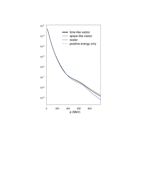
FIG. 2.: We show the different momentum distributions as defined in eq. (54). The following distributions are presented: the time-like vector distribution (solid line), the space-like vector distribution (dash-dotted line), the scalar distribution (dashed line), and the time-like vector distribution with the P-waves put to zero (dash-double-dotted line).

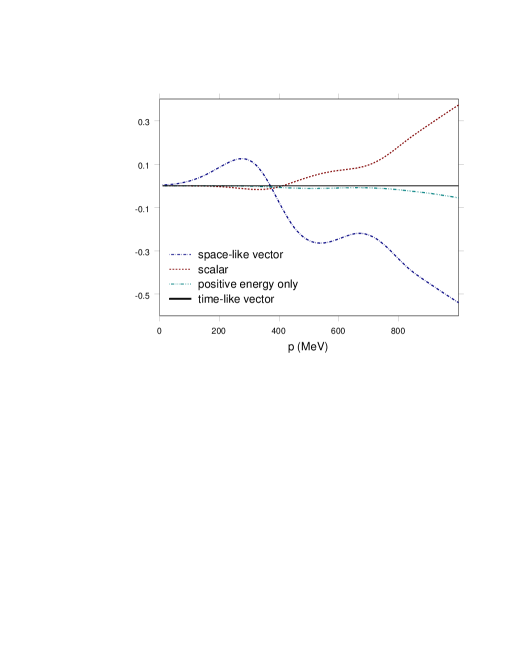
FIG. 3.: We plot the ratio $R=\frac{n_{x}-n_{TV}}{n_{TV}}$. The curves indicate the same distributions as in Fig. 2.

From the hadronic tensor, one can compute the response functions by picking the appropriate values of the indices $\mu,\nu$ and evaluating the traces. The explicit expressions for the responses are given in appendix B. In this process, not only the time-like vector momentum distribution, but also the scalar and the space-like momentum distributions enter in the evaluation of the response functions. In order to give an idea about the amount of interference that is possible in the response functions, we have plotted the three different momentum distributions in Figs. 2 and 3. In Fig. 2, we show the time-like vector distribution (solid line), the space-like vector distribution (dash-dotted line), and the scalar distribution (dashed line). In addition, we have plotted the time-like vector distribution with the P-waves put to zero (dash-double-dotted line). This would correspond to the non-relativistic momentum distribution. In Fig. 3, we show the ratio R, $R=\frac{n_{x}-n_{TV}}{n_{TV}}$, of the deviations of the different distributions from the time-like distribution to the time-like vector distribution. One can see clearly that both the space-like vector and scalar distributions deviate significantly from the time-like vector distribution, in the case of the space-like vector distribution, this happens already for rather small momenta. For increasing momenta, the interference effects grow considerably, until they reach 30 % to 50%. In contrast, the effect of the P waves in the time-like vector distribution is small, and increases only slightly for very high momenta, $p>800$ MeV/c. This is as expected, as the P waves do not interfere with S or D waves in this case, and their normalization is too small to make them significant by themselves, compared to the S wave or D wave contribution.

III Comparison of different approaches to relativity

In this section, we compare the results of a plane wave calculation of the $D(e,e^{\prime}p)n$ reaction in the framework of the Gross equation [9, 2] (Model R) with a calculation using a non-relativistic nucleon-nucleon potential, namely the Argonne V18 potential [14], and the full relativistic current operator (Model A1). For an overview of all employed models and naming conventions, see appendix A. Both models give a very good fit to the $NN$ scattering data. At the high energy and momentum transfer we consider here, the Plane Wave Impulse Approximation and the Plane Wave Born Approximation become almost identical, they differ by 2% or 3% at most. In order to be consistent with the analytic formulas presented in the previous section and in the appendix, the calculations we show are done in PWIA. We perform our comparison for the basic observable, the differential cross section.

FIG. 4.: The differential cross section for the ${}^{2}H(e,e^{\prime}p)n$ reaction is shown for fixed 3-momentum transfer $q=1.4$ GeV/c and different values of the fixed energy transfers $\omega$: 0.61 GeV (a), 0.75 GeV (b), and 0.94 GeV (c). The kinematic conditions in the middle panels correspond to quasi-free conditions. The solid line shows the result of the fully relativistic calculation (Model R), the dashed line shows the result of the calculation with the Argonne V18 wave function and the full relativistic current operator (Model A1), and the dash-dotted line shows the result of the calculation with the Argonne V18 wave function and the strict non-relativistic reduction of the current operator (Model NR).

In Figs. 4 and 5, we compare the fully relativistic, covariant results (Model R) with the results for the Argonne V18 wave function in conjunction with the full relativistic current operator (Model A1). We have also added a curve showing the results obtained with the Argonne V18 wave function and the traditional, strictly non-relativistic current operator (Model NR), in order to give an idea of the actual size of relativistic effects in the current. In the first figure, we have fixed the transferred momentum, $q$, to $q=1.4$ GeV/c, and the transferred energy, $\omega$, to a value corresponding to the quasi-elastic peak, $\omega=0.75$ GeV (middle panel), to a value below the quasi-elastic peak, $\omega=0.61$ GeV (top panel), and to a value above the quasi-elastic peak, $\omega=0.94$ GeV (bottom panel). This choice corresponds to values of the $y$-scaling variable of $y=0$ GeV/c, $y=-0.2$ GeV/c, and $y=0.2$ GeV/c. The $y$ variable is defined as the negative minimal missing momentum, for details, see e.g. [15]. The solid line shows the fully relativistic calculation, the dashed line shows the calculation with the relativistic current operator and the AV18 wave function, and the dash-dotted line shows the the calculation with the traditional non-relativistic reduction of the current and the AV18 wave function. We start our discussion with the lowest energy transfer, $\omega=0.61$ GeV. One sees that the fully relativistic calculation and the AV18 with full relativistic current are relatively close to each other, with the fully relativistic result a bit lower for missing momenta around $400$ MeV/c. The result obtained with the non-relativistic current operator is larger than the relativistic curves. For the quasi-free kinematics (middle panel), the fully relativistic calculation and the AV18 plus full relativistic current agree quite nicely, with the fully relativistic curve being slightly lower for momenta around $350$ MeV/c and then being slightly higher for momenta higher than $500$ MeV/c. The non-relativistic result is significantly higher for all missing momenta. This trend continues for the kinematics above the quasi-elastic peak (lower panel), where the difference between non-relativistic and relativistic curves increases again. This is to be expected, as one of the basic assumptions of the strictly non-relativistic reduction is that the transferred energy is much smaller than the transferred momentum. This condition is fulfilled to a certain extent below the quasi-elastic peak, but not on or above it. The fully relativistic result and the AV18 plus full relativistic current agree for missing momenta up to $400$ MeV/c, then the AV18 result drops off a bit. This difference is the largest between these two calculations which we have encountered so far, and it is logical that it should arise where it does: certainly, relativistic effects are expected to be strongest for situations where both energy and momentum transfer are large, and for high missing momenta, which correspond in the absence of final state interactions to the initial momentum of the nucleon in the nucleus. It is logical to expect any relativistic effect in the nuclear dynamics to show up at high missing momenta. Below, we will discuss the relativistic effects surpassing kinematics and current.

FIG. 5.: The differential cross section for the ${}^{2}H(e,e^{\prime}p)n$ reaction is shown for fixed kinetic energy, $T_{kin}=1$ GeV, of the outgoing proton in parallel and perpendicular kinematics. The curves have the same meaning as in Fig. 4.

In order to get a different view, we also show the same results for a different kinematic situation: now, we fix the kinetic energy of the outgoing proton to 1 GeV, and consider parallel and perpendicular kinematics. The results are shown in Fig. 5. For parallel kinematics (top panel), the fully relativistic result and the AV18 plus full relativistic current result coincide for missing momenta below $300$ MeV/c, for higher missing momenta, the fully relativistic curve is a bit lower. The non-relativistic result differs from the other results already at the lowest missing momenta, but the difference is comparatively small in these kinematics, the momentum transfer increases very quickly, so that the relation $\omega<<q$ is roughly applicable, as in the case of Fig. 4, top panel. In perpendicular kinematics, the fully relativistic result and the AV18 plus exact current result agree very nicely up to $p_{m}=450$ MeV/c, for higher missing momenta, the two calculations start to diverge, leading to a difference similar to the one observed for the highest energy transfer in the fixed q kinematics.

To summarize the results of our comparison so far, we have seen that there is very good overall agreement between the fully relativistic result (Model R) and the AV18 plus full relativistic current result (Model A1), with some slight deviations at higher missing momenta, $p_{m}\geq 450$ MeV/c, especially for energy transfers $\omega$ comparable to q. The calculation with the AV18 wave function and the non-relativistic reduction of the current (Model NR) differs from the relativistic results considerably, starting from the lowest missing momenta. In the light of these results, it is fair to say that the bulk of the relativistic effects in the few GeV region does stem from the current, as conjectured in [1].

FIG. 6.: The momentum distribution n(p) for the deuteron is shown for several wave function models. The solid line shows the Bonn result, the dashed line shows the Paris result, the dash-dotted line shows the CD Bonn result, and the long dashed line shows the Argonne V18 result. The short-dashed line shows the momentum distribution calculated with the S wave and D wave of the Gross wave function.

In order to ascertain the influence of relativity in contrast to the influence of the modeling of the $NN$ interaction properly, we carry out an additional comparison. We take a parameterization of the S wave and D wave part of the Gross wave function, and use this together with the full relativistic current (Model G1). Whether the model for the $NN$ interaction is relativistic or not, this choice alone does not specify the model. The data constrain the deuteron wave function somewhat, but it is well known that for higher momenta, where the D wave is dominant, different models make different predictions. E.g. the Bonn [16] and the Paris [17] wave functions are both non-relativistic, but differ greatly in their D wave content. In our comparison, we are interested in the different treatment of relativity, and want to eliminate differences due to the difference in the $NN$ interaction modeling. We therefore show a plot of the momentum distribution as given by eq. (24) of several non-relativistic models, and also plot the momentum distribution obtained with the S wave and D wave of the Gross wave function. We omit the P waves here in order to compare the same quantity, the different normalization induced by this has been taken into account. As seen in Fig. 6, all wave function models agree for momenta up to 300 MeV/c, and then start to diverge. The two Bonn potential curves, Bonn [16] and CD Bonn [18], are lower than Paris, Argonne V18 and the Gross wave function. The latter three are fairly close, with the Paris and Argonne V18 slightly higher than the Gross wave function. This means that our comparison between the fully relativistic calculation (Model R) and the Argonne V18 with the full relativistic current (Model A1) is meaningful, as the differences in these calculations should arise mainly from the different treatment of relativity, not from the differences in the wave function. Note that a comparison of the fully relativistic calculation with one of the Bonn potential wave functions plus full relativistic current would not have achieved that.

FIG. 7.: The differential cross section for the ${}^{2}H(e,e^{\prime}p)n$ reaction is shown for fixed 3-momentum transfer $q=1.4$ GeV/c and different values of the fixed energy transfers $\omega$: 0.61 GeV (a), 0.75 GeV (b), and 0.94 GeV (c). The kinematic conditions in the middle panels correspond to quasi-free conditions. The solid line shows the result of the fully relativistic calculation (Model R), the dashed line shows the result of the calculation with the Argonne V18 wave function and the full relativistic current operator (Model A1), and the dash-dotted line shows the result of the calculation with the Gross S wave and D wave plus the full relativistic current operator (Model G1).

In order to be as precise as possible in our investigation of relativistic effects, we compare the fully relativistic calculation (Model R), the Argonne V18 plus full relativistic current (Model A1), and the Gross S wave and D wave plus full relativistic current (Model G1). The curves are shown in Figs. 7 and 8. The kinematic conditions are the same as in Figs. 4 and 5. First, we discuss the results for fixed energy and momentum transfer. Due to the fact that the momentum distribution calculated with the Gross wave function is slightly lower than the Argonne V18 momentum distribution, the Gross S+D plus full relativistic current results are slightly lower than the AV18 plus full relativistic current results. This improves the agreement with the full relativistic calculation for the lowest energy transfer, $\omega=0.61$ GeV for momenta less than 400 MeV/c. For higher missing momenta, the deviation from the full relativistic calculations increases a bit, although not significantly, leaving a little more room for genuine relativistic nuclear dynamics effects. In Fig. 8, we show the results for fixed kinetic energy of the outgoing proton. For parallel kinematics, the use of the Gross S and D waves plus full relativistic current results improves the agreement with the fully relativistic calculation, the two curves differ only slightly. For perpendicular kinematics, all three curves agree nicely for missing momenta up to 350 MeV/c, then the Gross S and D wave plus full relativistic current calculation differs from the full calculation a bit more than the corresponding AV18 curve.

FIG. 8.: The differential cross section for the ${}^{2}H(e,e^{\prime}p)n$ reaction is shown for fixed kinetic energy, $T_{kin}=1$ GeV, of the outgoing proton in parallel and perpendicular kinematics. The curves have the same meaning as in Fig. 7.

So, overall, we have very good agreement between the fully relativistic calculation and the AV18 or Gross S and D wave plus full relativistic current. In contrast to this, a calculation with the strict non-relativistic reduction of the electromagnetic current disagrees markedly with the relativistic results. In the remainder of this paper, we discuss the possible sources for the remaining small discrepancies at higher missing momenta.

A P-wave contributions

One genuinely relativistic effect that cannot be taken care of by the electromagnetic current is the emergence of P waves in the deuteron wave function. They arise naturally from the lower spinor components, and there is a P-wave singlet and a P-wave triplet contribution, see e.g. [19]. Although their normalization is extremely small compared to the S-wave and the D-wave, they can play an important role, e.g. in the calculation of the elastic deuteron form-factors, where they shift the location of the minimum of $B(Q^{2})$ by a considerable amount [20]. How important are they for $(e,e^{\prime}p)$ reactions? We investigate this question by switching off the P-wave contribution and comparing the full result (Model R) with the result without P-waves (Model RSD) in Figs. 9 and 10. Overall, the differences between the full calculation and the calculation without P waves are very small. In the fixed q and $\omega$ kinematics, the two curves coincide for the lowest energy transfer of 0.61 GeV, and barely differ for $\omega=0.75$ GeV. Only for the highest energy transfer of 0.94 GeV, the P waves have an effect, their inclusion slightly increases the result. We would like to point out that this is due to interference between the P waves and the S and D waves. The contribution of the P waves alone is approximately two orders of magnitude smaller than the contribution of S and D waves, so the interference effects must be quite large in order to be visible. In Fig. 10, in parallel kinematics (top panel), the two curves barely differ. It is interesting, though, to see that the interference in this case is destructive, leading to a slightly enhanced result when the P waves are omitted. In perpendicular kinematics, the omission of the P waves lowers the result slightly for missing momenta higher than 400 MeV/c. In each case, when comparing with Figs. 4 and 5 and with Figs. 7 and 8, one sees that the P wave contribution explains a part of the difference between the fully relativistic result and the other calculations, but not all of it. Another important aspect for calculations at higher missing momenta are off-shell prescriptions, they will be discussed in the next section.

FIG. 9.: The differential cross section for the ${}^{2}H(e,e^{\prime}p)n$ reaction is shown for fixed 3-momentum transfer $q=1.4$ GeV/c and different values of the fixed energy transfers $\omega$: 0.61 GeV (a), 0.75 GeV (b), and 0.94 GeV (c). The kinematic conditions in the middle panels correspond to quasi-free conditions. The solid line shows the result of the fully relativistic calculation (Model R), the dashed line shows the result of the fully relativistic calculation without the P waves (Model RSD).

FIG. 10.: The differential cross section for the ${}^{2}H(e,e^{\prime}p)n$ reaction is shown for fixed kinetic energy, $T_{kin}=1$ GeV, of the outgoing proton in parallel and perpendicular kinematics. The curves have the same meaning as in Fig. 9.

One additional remark is in order: although the P-waves are only of marginal importance for the calculation of the differential cross section and the large responses, they may play a more important role in the calculation of single or double polarization observables, by interfering with one of the larger contributions. Similar situations arise e.g. when considering the second-order convective spin-orbit contribution to the transverse-transverse response function, which is considerable due to the interference with the magnetization current, the largest current component that cannot contribute to the transverse-transverse response function otherwise [1]; or when considering the contribution of the spin-orbit final state interaction to the fifth response function, which allows for a large interference of the two dominant components of the current that is not present otherwise [7]. In general, one needs to be careful in situations where a change of the spin structure will allow for a new, large contribution. In these situations, it is advisable to take a close look at the relevant Clebsch-Gordan coefficients and to determine if additional important contributions could arise from the presence of P-waves.

B Off-shell effects

Whenever one applies the one-body electromagnetic current operator not to a free nucleon, but to a nucleon bound in the nucleus, one needs to introduce an off-shell prescription. Nucleons in the nucleus are bound and therefore off-shell; they do not fulfill the same energy-momentum relations as free nucleons. Currently, there exists no microscopic description of this off-shell behavior that can be applied for a wide range of kinematic conditions — there are only ad hoc prescriptions, which lead to differing results for certain kinematics [21, 22, 23]. The variations tend to increase with increasing momentum of the initial nucleon - the higher its momentum, the further it is off-shell. The fully relativistic calculation (Model R, Model RSD) uses a more sophisticated off-shell prescription, which takes into account the actual kinematics. In the calculation with the non-relativistic wave functions and the exact form of the current operator, we have chosen the popular ansatz of employing the “on-shell form” of the current. However, these are specific choices among an infinite number of prescriptions. We will quantify the theoretical uncertainty due to these choices in the following. It is easy to see why there are, in principle, infinitely many possibilities to choose an off-shell prescription. Consider the case of non-relativistic PWIA, and of factorization holding there, i.e. we are investigating the off-shell effects in the framework of non-relativistic wave function and full current operator now. Due to the factorization, the cross section can be described by the product of momentum distribution and off-shell electron-proton cross section, see eq. (20). For a free nucleon, one can write down the $ep$ cross section, and then rewrite it using simple algebra, that in general will employ the on-shell energy momentum relation for the free nucleon. On-shell, all these ways of writing the $ep$ cross section are equivalent - off-shell, they differ, and of course there is no way to identify a single expression as the correct one. E.g., one obtains different versions of the off-shell $ep$ cross section if one starts out from the one-body current in the form given in eq. (12), or if one uses the Gordon decomposition on the current. This is precisely how deForest [21] obtained his off-shell prescription cc1 (current like in eq. (12)) and cc2 (Gordon decomposition applied to the current). At first sight, the situation might look rather grim, however, things are not as bad as one might assume. In the following, we compare the employed off-shell prescriptions. In eq. (11), we gave the expressions for the single nucleon responses in terms of the $\xi$s, as they have been used in the calculations shown above (Models A1 and G1), and also in terms of $W_{1},W_{2}$ (Model A2). This latter form was obtained by doing some algebra involving the on-shell kinematic relations, and therefore constitutes a different off-shell prescription. In Fig. 11, top panel, we show the ratio of the $ep$ cross section calculated with the $\xi$s, called off-shell prescription 1, and with $W_{1},W_{2}$, referred to as off-shell prescription 2. The curves show the ratios for the kinematic settings discussed in this paper. One sees that, according to expectations, the off-shell prescriptions agree for momenta below 200 MeV/c, and then start to diverge. At the highest missing momenta considered here, the deviations range from 10% to 25%. At the intermediate momenta, the typical deviation from 1 is about 5 %. The largest deviations occur for $T_{kin}=1GeV$ in perpendicular kinematics (long dashed line), and for the $q=1.4$ GeV/c, $\omega=0.61$ GeV case (dash-dotted line). In the middle panel of Fig. 11, we show the ratio of off-shell prescription 1 and the off-shell prescription used in the covariant calculation, denoted as off-shell 3. The explicit formulas for off-shell 3 are given in appendix C. Again, the two off-shell prescriptions agree nicely for low missing momenta, and start to diverge for $p_{m}>200$ MeV/c. The deviations are large, almost 50 % at the highest missing momenta for $T_{kin}=1GeV$ in perpendicular kinematics, and also considerable at high missing momenta for $q=1.4$ GeV/c, $\omega=0.61$ GeV. In all other considered kinematics, the deviations do not exceed 5% even at the highest missing momenta. Note that the deviations from $1$ for the ratio of off-shell 2 to off-shell 3 are smaller than any of the ratios shown here, we have chosen to display the “extreme” cases here.

FIG. 11.: The upper panel shows the ratio of the off-shell electron proton cross sections calculated with prescription 1 and prescription 2. The different lines correspond to different kinematic settings: the solid line shows the ratio for $T_{kin}=1$ GeV, parallel kinematics, the long-dashed line for $T_{kin}=1$ GeV, perpendicular kinematics, the dash-dotted line for $q=1.4$ GeV/c, $\omega=0.61$ GeV, the dotted line for $q=1.4$ GeV/c, $\omega=0.75$ GeV, and the short-dashed line for $q=1.4$ GeV/c, $\omega=0.94$ GeV. In the middle and the lower panel, the different lines correspond to the same kinematic conditions as in the upper panel of this figure. The middle panel shows the ratio of the off-shell electron proton cross sections calculated with prescription 1 and prescription 3. The lower panel shows the ratio of the off-shell electron proton cross sections calculated with the full relativistic current and the strict non-relativistic reduction of the current for a fixed off-shell prescription, namely off-shell 1.

Although the off-shell prescriptions 1,2, and 3 are all relativistic, there remains an ambiguity in the choice of the off-shell kinematics. The scope of this paper was to investigate the treatment of relativistic effects, not the specific off-shell choices. However, our results give a good idea about the size of the uncertainties, and about the kinematic regions which are sensitive to them; whereas in parallel kinematics, the results are quite insensitive to the employed off-shell prescription, the results in perpendicular kinematics are more sensitive. Below missing momenta of $200$ MeV/c, off-shell ambiguities practically do not exist, and for $p_{m}<400$ MeV/c, they will in general not be larger than 10 %.

Sometimes, the full relativistic current is rejected as introducing off-shell contributions, and the claim is made that the non-relativistic reduction is preferable as it would avoid such ambiguities. This argument is not correct. Firstly, even the non-relativistic version of the current contains a dependence on the nucleon momentum, leading to terms proportional to the perpendicular momentum squared in the single nucleon responses, see eq. (37). On-shell, this momentum can be replaced with the energy by using the on-shell kinematic relations, and therefore one does have off-shell ambiguities even in this case. One might argue that the non-relativistic versions of the charge operator and the magnetization current do not contain any dependence on the initial nucleon momentum, and should therefore be free of off-shell ambiguities. Here, one needs to ask, however, if this feature was not bought at a too high price: the $ep$ cross sections calculated in the strict non-relativistic reduction differ from the relativistic version by 30 % to 80 %, and this discrepancy starts at $p_{m}=0$ MeV/c. We demonstrate this point by presenting the ratio of the relativistic to the non-relativistic $e-p$ cross section for one specific off-shell prescription, namely the on-shell form with the $\xi$s, referred to as off-shell 1, see Fig. 11, lower panel. Even though the off-shell effects in the full relativistic version of the current do introduce a theoretical uncertainty at higher missing momenta, the relativistic treatment is definitely superior to the non-relativistic version, where one knows that the results are off for all missing momentum values, and they are off up to a factor of 5.

IV Summary

The principal goal of this paper has been to investigate the origin of the relativistic effects in the electrodisintegration of the deuteron. Apart from the obviously relativistic kinematics, relativistic effects occur in the electromagnetic current operator and the nuclear dynamics. We have shown that calculations with a non-relativistic wave function and the fully relativistic current operator reproduce the fully relativistic calculation very well up to $400$ MeV/c of missing momentum in all kinematics. At the same time, a calculation with a non-relativistic wave function and a strictly non-relativistic current operator drastically fails to reproduce the relativistic results, in all kinematics and even for the lowest missing momenta.

We have shown that the relativistic effects in the nuclear dynamics, namely, the presence of P-waves, are rather small in the cross section. They do appear only in places where one would expect relativistic effects to show up, i.e. for high missing momenta, $p_{m}>400$ MeV/c and for energy transfers which are large and comparable to the momentum transfer. The remaining discrepancy that we found in a few kinematics for high missing momenta was shown to stem from the different off-shell prescriptions used in the two calculations.

Since [24] shows that the effects of bound state dynamical relativity are small also in heavier nuclei, the technique of [1] can reliably be applied to heavier nuclei, too.

These findings verify the conjecture of [1] that at energies of a few GeV, the bulk of the relativistic effects in electronuclear reactions stems from the current operator, and not from the nuclear dynamics.

A Overview over presented calculations: notation

For the convenience of the reader, we list all calculations and assign a short name for them:

wave function	responses/off-shell prescription	description	name
Gross wave function;	as in appendix B,	fully relativistic,	Model R
S, D, P waves	off-shell 3	covariant calculation
Gross wave function;	as in appendix B,	fully relativistic,	Model RSD
S, D waves	off-shell 3	covariant calculation
Argonne V18;	as in eq. (33),	AV18 plus full	Model A1
S, D waves	with the $\xi$, off-shell 1	relativistic current
Argonne V18;	as in eq. (33),	AV18 plus full	Model A2
S, D waves	with $W_{1},W_{2}$, off-shell 2	relativistic current
Gross wave function;	as in eq. (33),	Gross S and D wave function	Model G1
S, D waves	with the $\xi$, off-shell 1	and full relativistic current
Argonne V18;	as in eq. (37),	AV18 plus strictly	Model NR
S, D waves	with the $\xi$, off-shell 1	non-relativistic current

B Fully relativistic nuclear responses

Here, the explicit analytic expressions for the nuclear response functions using the off-shell prescription of the fully relativistic, covariant calculation are given:

$$R_{L} = \frac{1}{8\pi}\,\frac{q^{2}}{Q^{2}}\,\{(C_{1}^{TV}n_{TV}(p)+C_{1}^{SV}n_{SV}(p)+C_{1}^{S}n_{S}(p))$$ (B3)

$$+C_{2}^{SV}n_{SV}(p)\,[(M_{d}-E_{p})\frac{q}{Q}-\frac{\omega}{Q}p_{z}]^{2}$$

$$+(C_{3}^{TV}n_{TV}(p)+C_{3}^{SV}n_{SV}(p))\,2M_{d}\,\frac{q}{Q}\,[(M_{d}-E_{p})\frac{q}{Q}-\frac{\omega}{Q}p_{z}]\}$$

$$R_{T} = \frac{1}{8\pi}\,\,\{-2\,(C_{1}^{TV}n_{TV}(p)+C_{1}^{SV}n_{SV}(p)+C_{1}^{S}n_{S}(p))$$ (B5)

$$+C_{2}^{SV}n_{SV}(p)\,\,p_{\perp}^{2}\}$$

$$R_{TT} = -\frac{1}{8\pi}\,\,C_{2}^{SV}n_{SV}(p)\,\,p_{\perp}^{2}\,\cos(2\varphi)$$ (B6)

$$R_{TL} = \frac{1}{8\pi}\,\frac{q}{Q}\,\{C_{2}^{SV}n_{SV}(p)\,2\sqrt{2}\,[(M_{d}-E_{p})\frac{q}{Q}-\frac{\omega}{Q}p_{z}]\,p_{\perp}\cos(\varphi)$$ (B8)

$$+(C_{3}^{TV}n_{TV}(p)+C_{3}^{SV}n_{SV}(p))\,2\sqrt{2}\,M_{d}\,\frac{q}{Q}\,p_{\perp}\cos(\varphi)\}$$

The coefficients $C$ of the time-like vector, space-like vector, and scalar momentum distributions are given by:

$$C_{1}^{TV} = \frac{\Delta-M_{d}^{2}}{4\,m^{2}\,M_{d}^{2}}\,\{(M_{d}^{2}+\Delta)(F_{1}^{2}(Q^{2})+\tau F_{2}^{2}(Q^{2}))$$ (B10)

$$+2M_{d}\,\omega\,F_{1}(Q^{2})\,(F_{1}(Q^{2})+F_{2}(Q^{2}))-\frac{M_{d}\,\Delta\,\omega}{2\,m^{2}}F_{2}^{2}(Q^{2})\}$$

$$C_{2}^{TV} = 0$$ (B11)

$$C_{3}^{TV} = \frac{M_{d}^{2}-\Delta}{2\,m^{2}\,M_{d}^{2}}(F_{1}^{2}(Q^{2})+\tau F_{2}^{2}(Q^{2}))$$ (B12)

$$C_{4}^{TV} = 0\,$$ (B13)

where $\Delta=p_{1}^{2}-m^{2}=M_{d}^{2}-2M_{d}E_{p}$ measures the “off-shellness” of the bound nucleon.

$$C_{1}^{SV} = -\left(1-\frac{M_{d}^{2}}{4\,m^{2}}\right)(F_{1}^{2}(Q^{2})+\tau F_{2}^{2}(Q^{2}))-2\tau F_{1}(Q^{2})(F_{1}(Q^{2})+F_{2}(Q^{2}))$$ (B17)

$$+\frac{\Delta}{2\,m^{2}}F_{1}(Q^{2})F_{2}(Q^{2})-\frac{\Delta^{2}}{8\,m^{4}}F_{2}^{2}(Q^{2})+\frac{\Delta^{2}}{4\,m^{2}\,M_{d}^{2}}(F_{1}^{2}(Q^{2})+\tau F_{2}^{2}(Q^{2}))$$

$$-\frac{\Delta^{2}\omega}{8\,m^{4}\,M_{d}}F_{2}^{2}(Q^{2})+\frac{\Delta\omega}{2\,m^{2}\,M_{d}}(F_{1}^{2}(Q^{2})+2F_{1}(Q^{2})F_{2}(Q^{2})-\frac{M_{d}^{2}}{4\,m^{2}}F_{2}^{2}(Q^{2}))$$

$$+\frac{M_{d}\,\omega}{2\,m^{2}}F_{1}(Q^{2})(F_{1}(Q^{2})+F_{2}(Q^{2}))$$

$$C_{2}^{SV} = \frac{2}{m^{2}}\,(F_{1}^{2}(Q^{2})+\tau F_{2}^{2}(Q^{2}))$$ (B18)

$$C_{3}^{SV} = -\frac{\Delta+M_{d}^{2}}{2\,m^{2}\,M_{d}^{2}}(F_{1}^{2}(Q^{2})+\tau F_{2}^{2}(Q^{2}))$$ (B19)

$$C_{4}^{SV} = 0$$ (B20)

$$C_{1}^{S} = F_{1}^{2}(Q^{2})-\tau F_{2}^{2}(Q^{2})-2\tau F_{1}(Q^{2})F_{2}(Q^{2})-\frac{\Delta}{2\,m^{2}}F_{1}(Q^{2})F_{2}(Q^{2})$$ (B21)

$$C_{2}^{S} = 0$$ (B22)

$$C_{3}^{S} = 0$$ (B23)

$$C_{4}^{S} = 0$$ (B24)

Note that the responses given here are to be inserted into eq. (3) for the cross section in the lab frame. The responses $\tilde{R}$ used in [10] in eq. (95) are connected to these responses in the following way:

$$R_{L} = \frac{2\pi^{2}}{m^{2}}\frac{W}{M_{T}}\frac{q^{2}}{Q^{2}}\tilde{R}_{L}$$ (B25)

$$R_{T} = \frac{2\pi^{2}}{m^{2}}\frac{W}{M_{T}}\tilde{R}_{T}$$ (B26)

$$R_{TT} = \frac{2\pi^{2}}{m^{2}}\frac{W}{M_{T}}\tilde{R}_{TT}\cos(2\varphi)$$ (B27)

$$R_{TL} = \frac{2\pi^{2}}{m^{2}}\frac{W}{M_{T}}\frac{q}{Q}\tilde{R}_{TL}\cos(\varphi)$$ (B28)

Here, $W$ indicates the invariant mass of the final state, and $M_{T}$ is the target mass.

C Single nucleon off-shell responses

In the case of vanishing P-wave contributions, the different momentum distributions coincide:

$$n_{TV}(p)=n_{SV}(p)=n_{S}(p)\equiv n^{+}(p)=u^{2}(p)+w^{2}(p)$$ (C1)

Note that the normalization condition of the Gross wave function as given in eq. (55) differs from the one employed for the Bonn and Paris wave function, eq. (25). The different normalizations have of course been taken into account when we compared the two results. For vanishing P-waves, the responses factorize, and the resulting off-shell single nucleon responses are called “off-shell 3” in the text. For the convenience of the reader, they are given here explicitly:

$$R_{L}^{sn,no\,p} = \frac{1}{8\pi}\,\frac{q^{2}}{Q^{2}}\,\{-2\tau(F_{1}(Q^{2})+F_{2}(Q^{2}))^{2}+\frac{\Delta^{2}}{2\,m^{2}\,M_{d}^{2}}(F_{1}^{2}(Q^{2})+\tau F_{2}^{2}(Q^{2}))-\frac{\Delta^{2}}{8\,m^{4}}F_{2}^{2}(Q^{2})$$ (C5)

$$-\frac{\Delta^{2}\,\omega}{4\,m^{4}\,M_{d}^{2}}\,F_{2}^{2}(Q^{2})+\frac{\Delta\,\omega}{m^{2}\,M_{d}}F_{1}(Q^{2})(F_{1}(Q^{2})+F_{2}(Q^{2}))$$

$$+\frac{2}{m^{2}}(F_{1}(Q^{2})+F_{2}(Q^{2}))^{2}[(M_{d}-E_{p})\frac{q}{Q}-\frac{\omega}{Q}p_{z}]^{2}$$

$$-\frac{\Delta}{m^{2}\,M_{d}^{2}}(F_{1}^{2}(Q^{2})+\tau F_{2}^{2}(Q^{2}))\,2M_{d}\,\frac{q}{Q}\,[(M_{d}-E_{p})\frac{q}{Q}-\frac{\omega}{Q}p_{z}]\}$$

$$R_{T}^{sn,no\,p} = \frac{1}{8\pi}\,\{4\tau(F_{1}(Q^{2})+F_{2}(Q^{2}))^{2}-\frac{\Delta}{m^{2}\,M_{d}^{2}}(F_{1}^{2}(Q^{2})+\tau F_{2}^{2}(Q^{2}))$$ (C8)

$$+\frac{\Delta^{2}}{4\,m^{4}}F_{2}^{2}(Q^{2})+\frac{\Delta^{2}\,\omega}{2\,m^{4}M_{d}}F_{2}^{2}(Q^{2})-\frac{2\Delta\omega}{m^{2}\,M_{d}^{2}}F_{1}(Q^{2})(F_{1}(Q^{2})+F_{2}(Q^{2}))$$

$$+\frac{2}{m^{2}}(F_{1}^{2}(Q^{2})+\tau F_{2}^{2}(Q^{2}))p_{\perp}^{2}\}$$

$$R_{TT}^{sn,no\,p} = -\frac{1}{8\pi}\,\frac{2}{m^{2}}(F_{1}^{2}(Q^{2})+\tau F_{2}^{2}(Q^{2}))p_{\perp}^{2}\,\cos(2\varphi)$$ (C9)

$$R_{TL}^{sn,no\,p} = \frac{1}{8\pi}\,\frac{q}{Q}\,\{\frac{2}{m^{2}}(F_{1}^{2}(Q^{2})+\tau F_{2}^{2}(Q^{2}))\,2\sqrt{2}\,[(M_{d}-E_{p})\frac{q}{Q}-\frac{\omega}{Q}p_{z}]\,p_{\perp}$$ (C11)

$$-\frac{\Delta}{m^{2}\,M_{d}^{2}}(F_{1}^{2}(Q^{2})+\tau F_{2}^{2}(Q^{2}))\,2\sqrt{2}\,M_{d}\,\frac{q}{Q}p_{\perp}\}\cos(\varphi)$$

REFERENCES

- [1] S. Jeschonnek and T.W. Donnelly, Phys. Rev. C 57, 2438 (1998).
- [2] J. W. Van Orden, N. Devine, and F. Gross, Phys. Rev. Lett. 75, 4369 (1995).
- [3] E. Hummel and J. A. Tjon, Phys. Rev. C 49, 21 (1994).
- [4] J. E. Amaro, J. A. Caballero, T. W. Donnelly, A. M. Lallena, E. Moya de Guerra, and J. M. Udías, Nucl. Phys. A602, 263 (1996).
- [5] J. E. Amaro, J. A. Caballero, T. W. Donnelly, and E. Moya de Guerra, Nucl. Phys. A611, 163 (1996).
- [6] J. E. Amaro and T. W. Donnelly, Ann. Phys. 263, 56 (1998).
- [7] S. Jeschonnek and T.W. Donnelly, Phys. Rev. C 59, 2676 (1999).
- [8] A. S. Raskin and T. W. Donnelly, Ann. of Phys. 191, 78 (1989).
- [9] F. Gross, Phys. Rev. 186, 1448 (1969); F. Gross, Phys. Rev. D 10, 223 (1974); F. Gross, Phys. Rev. C 26, 2203 (1982).
- [10] V. Dmitrasinovic and F. Gross, Phys. Rev. C 40, 2479 (1989).
- [11] A. Picklesimer and J. W. Van Orden, Phys. Rev. C 40, 290 (1989).
- [12] J. A Caballero, T. W. Donnelly, E. Moya de Guerra, J. M. Udías, Nucl. Phys. A632, 323 (1998).
- [13] S. Gardner and J. Piekarewicz, Phys. Rev. C 50, 2822 (1994).
- [14] R. B. Wiringa, V. G. J. Stoks, and R. Schiavilla, Phys. Rev. C 51, 38 (1995).
- [15] D. B. Day, J. S. McCarthy, T. W. Donnelly, and I. Sick, Annu. Rev. Nucl. Part. Sci. 40, 357 (1990).
- [16] R. Machleidt, K. Holinde and C. Elster, Phys. Rep. 149, 1 (1987).
- [17] M. Lacombe, B. Loiseau, R. Mau, J. Côtè, P. Pirès and R. Tourreil, Phys. Lett. B101, 139 (1981).
- [18] R. Machleidt, F. Sammarruca, and Y. Song, Phys. Rev. C 53, 1483 (1996).
- [19] W. W. Buck and F. Gross, Phys. Rev. D 20, 2361 (1979).
- [20] J. W. Van Orden, N. Devine, and F. Gross, Phys. Rev. Lett. 75 4369 (1995).
- [21] T. de Forest Jr., Nucl.Phys. A392, 232 (1983).
- [22] H. W. L. Naus, S. J. Pollock, J. H. Koch, and U. Oelfke, Nucl. Phys. A509, 717 (1990).
- [23] J. A. Caballero, T. W. Donnelly, and G. I. Poulis, Nucl. Phys. A555, 709 (1993).
- [24] A. Picklesimer, J. W. Van Orden, and S. J. Wallace, Phys. Rev. C 32 1312 (1985).