Nuclear Skins and Halos in the Mean-Field Theory

Abstract

Nuclei with large neutron-to-proton ratios have neutron skins, which manifest themselves in an excess of neutrons at distances greater than the radius of the proton distribution. In addition, some drip-line nuclei develop very extended halo structures. The neutron halo is a threshold effect; it appears when the valence neutrons occupy weakly bound orbits. In this study, nuclear skins and halos are analyzed within the self-consistent Skyrme-Hartree-Fock-Bogoliubov and relativistic Hartree-Bogoliubov theories for spherical shapes. It is demonstrated that skins, halos, and surface thickness can be analyzed in a model-independent way in terms of nucleonic density form factors. Such an analysis allows for defining a quantitative measure of the halo size. The systematic behavior of skins, halos, and surface thickness in even-even nuclei is discussed.

]

I Introduction

One of the main frontiers of nuclear science today is the physics of radioactive nuclear beams (RNB). Experiments with beams of unstable nuclei make it possible to look closely into many unexplored regions of the periodic chart and many unexplored aspects of the nuclear many-body problem [1, 2, 3, 4, 5].

Prospects for new physics, especially on the neutron-rich side of the beta-stability valley, have generated considerable excitement in the low-energy nuclear physics community. Neutron-rich nuclei offer an opportunity to study the wealth of phenomena associated with the closeness of the particle threshold: particle emission (ionization to the continuum) and characteristic behavior of cross sections [6, 7], existence of soft collective modes and low-lying transition strength [8, 9, 10, 11, 12, 13], and dramatic changes in shell structure and various nuclear properties in the sub-threshold regime [14, 15, 16].

A very interesting aspect of nuclei far from stability is an increase in their radial dimension with decreasing particle separation energy [17, 18, 19, 20, 21]. Extreme cases are halo nuclei – loosely bound few-body systems with about thrice more neutrons than protons. The halo region is a zone of weak binding in which quantum effects play a critical role in distributing nuclear density in regions not classically allowed.

Halo nuclei, with their intricate topologies, are symbols of RNB physics. The very weak binding of the outermost neutrons leading to a rather good decoupling of halo from the core simplifies many aspects of underlying nuclear structure and reaction mechanism. Theoretically, the weak binding and corresponding closeness of the particle continuum, together with the need for the explicit treatment of few-body dynamics, makes the subject of halos both extremely interesting and difficult [3].

In the heavy neutron-rich nuclei, where the concept of mean field is better applicable, an a priori separation into core and halo nucleons seems less justified. However, the fact that there are far more neutrons than protons in these nuclei implies the existence of the neutron skin (i.e., an excess of neutrons at large distances). In addition, in neutron-rich weakly bound nuclei, one expects to see both the skin and the halo.

There is no consensus in the literature on how to define and parametrize skins and halos. A quantity which is often employed to characterize the spatial extension of neutron density is the difference between neutron and proton root mean square (rms) radii:

$$\Delta R_{np}\equiv\langle r_{n}^{2}\rangle-\langle r_{p}^{2}\rangle.$$ (1)

In normal nuclei, this quantity is known to vary between 0.1–0.2 fm [22, 23, 24, 25], but it increases significantly in neutron-rich systems due to both skin and halo effects.

Stimulated by recent experimental developments mainly in light nuclei, where some information on $\Delta R_{np}$ has been obtained [26, 27, 28, 29, 30] (see also the recent studies based on the giant dipole [31] and spin-dipole [32] resonance data and on antiprotonic levels [33, 34]), many theoretical papers with a focus on radii of neutron and proton density distributions appeared [35, 36, 37, 38, 39, 40, 41, 42, 43, 44, 45, 46, 47, 48, 49, 50, 51, 52, 53, 54, 55]. (For earlier works, see papers quoted in Ref. [25].) In most cases, theoretical studies were concerned with rms radii, and the skin was usually discussed in terms of quantity (1).

Unfortunately, the second moment of nucleonic density (the rms radius) provides a very limited characterization of the nucleonic distribution. In particular, since the parameter $\Delta R_{np}$ can be strongly influenced by weakly bound valence nucleons, i.e., by the shell structure, it is not able to properly describe the bulk radial behavior of drip-line nuclei. A powerful tool that allows a more detailed description is the Helm model, introduced in the context of electron scattering experiments [56, 57, 58]. In this model, the diffraction radius and surface thickness extracted from the density form factor are mainly sensitive to the nucleonic distribution in the surface region, and they are practically independent of shell fluctuations in the nuclear interior [59, 60, 61, 62, 63]. The robustness of the Helm model parameters, and their simple geometric interpretation, make this model a very attractive tool when characterizing density distributions.

The main goal of this study is to apply the Helm model to nucleonic densities calculated in the self-consistent mean-field theory. In the first part of this paper, it is demonstrated that by analyzing the nucleonic form factor one is able to define, in a model-independent way, contributions to proton and neutron radii coming from skins and halos. In the second part, we perform systematic calculations of skins and halos in spherical even-even nuclei and discuss their dependence on the model employed.

The material contained in this study is organized as follows. The analysis of nucleonic density based on the Helm model is outlined in Sec. II. Section III discusses the details of Hartree-Fock-Bogoliubov (HFB) and relativistic Hartree-Bogoliubov (RHB) models employed. The results of self-consistent calculations for diffraction radii, surface thickness, skins, and halos in spherical even-even nuclei are discussed in Sec. IV, together with the simple analysis based on the square-well model. Finally, Sec. V contains the main conclusions of this work.

II Spherical Helm Model

A key feature of the nucleonic density is the rms radius

$$R_{\rm rms}\equiv\sqrt{\langle r^{2}\rangle}=\sqrt{\frac{\int d^{3}\mathchoice{{\hbox{\boldmath$\displaystyle r$}}}{{\hbox{\boldmath$\textstyle r$}}}{{\hbox{\boldmath$\scriptstyle r$}}}{{\hbox{\boldmath$\scriptscriptstyle r$}}}\,r^{2}\rho(\mathchoice{{\hbox{\boldmath$\displaystyle r$}}}{{\hbox{\boldmath$\textstyle r$}}}{{\hbox{\boldmath$\scriptstyle r$}}}{{\hbox{\boldmath$\scriptscriptstyle r$}}})}{\int d^{3}\mathchoice{{\hbox{\boldmath$\displaystyle r$}}}{{\hbox{\boldmath$\textstyle r$}}}{{\hbox{\boldmath$\scriptstyle r$}}}{{\hbox{\boldmath$\scriptscriptstyle r$}}}\,\rho(\mathchoice{{\hbox{\boldmath$\displaystyle r$}}}{{\hbox{\boldmath$\textstyle r$}}}{{\hbox{\boldmath$\scriptstyle r$}}}{{\hbox{\boldmath$\scriptscriptstyle r$}}})}}.$$ (2)

Further characteristics are best deduced from the corresponding form factor

$$F(\mathchoice{{\hbox{\boldmath$\displaystyle q$}}}{{\hbox{\boldmath$\textstyle q$}}}{{\hbox{\boldmath$\scriptstyle q$}}}{{\hbox{\boldmath$\scriptscriptstyle q$}}})\equiv\int e^{i\mathchoice{{\hbox{\boldmath$\displaystyle qr$}}}{{\hbox{\boldmath$\textstyle qr$}}}{{\hbox{\boldmath$\scriptstyle qr$}}}{{\hbox{\boldmath$\scriptscriptstyle qr$}}}}\rho(\mathchoice{{\hbox{\boldmath$\displaystyle r$}}}{{\hbox{\boldmath$\textstyle r$}}}{{\hbox{\boldmath$\scriptstyle r$}}}{{\hbox{\boldmath$\scriptscriptstyle r$}}})d^{3}r.$$ (3)

For the spherical density distribution $\rho(r)$, the form factor $F(q)$ is spherical and can be expressed in the standard way:

$$F(q)=\int j_{0}(qr)\rho(r)r^{2}dr.$$ (4)

There are various ways to characterize the basic pattern of the nucleonic density. A choice that is straightforward and easy to use is provided by the Helm model [56, 57, 58]. Here, nucleonic density is approximated by a convolution of a sharp-surface density with radius $R_{0}$ with the Gaussian profile, i.e,

$$\rho^{\rm(H)}(\mathchoice{{\hbox{\boldmath$\displaystyle r$}}}{{\hbox{\boldmath$\textstyle r$}}}{{\hbox{\boldmath$\scriptstyle r$}}}{{\hbox{\boldmath$\scriptscriptstyle r$}}})=\int d^{3}\mathchoice{{\hbox{\boldmath$\displaystyle r$}}}{{\hbox{\boldmath$\textstyle r$}}}{{\hbox{\boldmath$\scriptstyle r$}}}{{\hbox{\boldmath$\scriptscriptstyle r$}}}^{\prime}\,f_{\rm G}(\mathchoice{{\hbox{\boldmath$\displaystyle r$}}}{{\hbox{\boldmath$\textstyle r$}}}{{\hbox{\boldmath$\scriptstyle r$}}}{{\hbox{\boldmath$\scriptscriptstyle r$}}}-\mathchoice{{\hbox{\boldmath$\displaystyle r$}}}{{\hbox{\boldmath$\textstyle r$}}}{{\hbox{\boldmath$\scriptstyle r$}}}{{\hbox{\boldmath$\scriptscriptstyle r$}}}^{\prime})\rho_{0}\Theta(R_{0}-|\mathchoice{{\hbox{\boldmath$\displaystyle r$}}}{{\hbox{\boldmath$\textstyle r$}}}{{\hbox{\boldmath$\scriptstyle r$}}}{{\hbox{\boldmath$\scriptscriptstyle r$}}}^{\prime}|),$$ (5)

where

$$f_{\rm G}(r)=\frac{1}{(2\pi)^{3/2}\sigma^{3}}e^{-\frac{r^{2}}{2\sigma^{2}}}.$$ (6)

The radius in $R_{0}$ in Eq. (5) is the diffraction (box equivalent) radius, and the folding width $\sigma$ in Eq. (6) models the surface thickness. The density $\rho_{0}$ is given by

$$\rho_{0}={3N\over{4\pi R_{0}^{3}}},$$ (7)

hence the Helm density $\rho^{\rm(H)}$ is normalized to the particle number $N$. The advantage of the Helm model is that folding becomes a simple product in Fourier space, thus yielding

$$F^{\rm(H)}(q)=\frac{3}{R_{0}q}j_{1}(qR_{0})e^{-\frac{\sigma^{2}q^{2}}{2}}.$$ (8)

It is obvious that the first zero of $F^{\rm(H)}(q)$ is uniquely related to the radius parameter $R_{0}$. The fit of this model parameter is thus trivial. We simply relate $R_{0}$ to the first zero of the realistic form factor $F(q)$, i.e.,

$$R_{0}=4.49341/q_{1},$$ (9)

where $q_{1}$ is the first zero of $F(q)$. This means that $R_{0}$ can be deduced from the diffraction minimum and this is why it is called a diffraction radius (or the box-equivalent radius). The surface thickness parameter, $\sigma$, can be computed by comparing the values of microscopic and Helm form factors, $F(q_{m})$ and $F^{\rm(H)}(q_{m})$, at the first maximum $q_{m}$ of $F(q)$, which gives

$$\sigma^{2}=\frac{2}{q_{m}^{2}}\ln\frac{3R_{0}^{2}j_{1}(q_{m}R_{0})}{R_{0}q_{m}F(q_{m})}.$$ (10)

We have now at our disposal three key parameters that characterize the microscopic nucleonic density: the rms radius $R_{\rm rms}$ as defined in Eq. (2), the diffraction radius $R_{0}$ from Eq. (9), and the surface thickness $\sigma$ given by Eq. (10). The Helm model has only two independent parameters, and thus its rms radius can be expressed in terms of $R_{0}$ and $\sigma$:

$$R^{\rm(H)}_{\rm rms}=\sqrt{\frac{3}{5}\left(R_{0}^{2}+5\sigma^{2}\right)}.$$ (11)

Furthermore, it is more natural to discuss radii which pertain to a geometrical size of the nucleus and, therefore, the prefactor $\sqrt{3/5}$ in Eq. (11) is rather inconvenient. We prefer to work with radii which we call here the geometric radii, defined as

$$R_{\rm geom} = \sqrt{\frac{5}{3}}R_{\rm rms},$$ (13)

$$R_{\rm Helm} = \sqrt{\frac{5}{3}}R^{\rm(H)}_{\rm rms}=\sqrt{\left(R_{0}^{2}+5\sigma^{2}\right)}.$$ (14)

With this definition, the geometric radius becomes the box-equivalent radius in the limit of a small surface thickness.

III Mean-field models

This section contains a very brief description of self-consistent models applied in this work. Since these models are standard, our discussion is limited to basic definitions and references.

A Hartree-Fock-Bogoliubov model

The HFB approach is a variational method which uses nonrelativistic independent-quasiparticle states as trial wave functions [64]. An independent-quasiparticle state is defined as a vacuum of quasiparticle operators which are linear combinations of particle creation and annihilation operators. In this work, instead of using the matrix representation corresponding to a set of single-particle creation operators numbered by the discrete index, we use the spatial coordinate representation [65, 66]. This is particularly useful when discussing spatial properties of the variational wave functions and the coupling to the particle continuum [66, 16].

In our HFB calculations, we employ the zero-range Skyrme interaction in the particle-hole channel. The total binding energy of a nucleus is obtained self-consistently from the energy functional [67]:

$${\cal E}={\cal E}_{\rm kin} + {\cal E}_{Sk}+{\cal E}_{Sk,ls}$$ (15)

$$+ {\cal E}_{C}+{\cal E}_{\rm pair}-{\cal E}_{\text{CM}},$$ (16)

where ${\cal E}_{\rm kin}$ is the kinetic energy functional, ${\cal E}_{Sk}$ is the Skyrme functional, ${\cal E}_{Sk,ls}$ is the spin-orbit functional, ${\cal E}_{C}$ is the Coulomb energy (including the exchange term), ${\cal E}_{\rm pair}$ is the pairing energy, and ${\cal E}_{\text{CM}}$ is the center-of-mass correction.

In this work, two Skyrme parametrizations are used: SkP [66] and SLy4 [68]. Both of these selected forces perform well concerning the total energies and radii. In particular, both SkP and SLy4 parametrizations have been shown to reproduce long isotopic sequences [68, 69].

In the particle-particle channel, we use the SkP parametrization in the HFB/SkP variant and the density-independent volume delta interaction in the HFB/SLy4 variant. The strength of the delta force was adjusted according to the prescription given in Refs. [68, 69]. For the details of the calculations, we refer the reader to Refs. [66, 16].

B Relativistic mean-field model

Relativistic mean-field theory has been proved to be a powerful tool in describing various aspects of nuclear structure [70]. The model explicitly includes mesonic degrees of freedom and describes the nucleons as Dirac particles. Nucleons interact in a relativistic covariant manner through the exchange of virtual mesons: the isoscalar scalar $\sigma$-meson, the isoscalar vector $\omega$-meson, and the isovector vector $\rho$-meson. The model is based on the one-boson exchange description of the nucleon-nucleon interaction. The starting point is the effective Lagrangian density [71, 72]

$${\cal L} = \bar{\psi}\left(i\gamma\cdot\partial-m\right)\psi$$ (20)

$$+\frac{1}{2}(\partial\sigma)^{2}-U(\sigma)-\frac{1}{4}\Omega_{\mu\nu}\Omega^{\mu\nu}+\frac{1}{2}m^{2}_{\omega}\omega^{2}$$

$$-\frac{1}{4}{\vec{\rm R}}_{\mu\nu}{\vec{\rm R}}^{\mu\nu}+\frac{1}{2}m^{2}_{\rho}\vec{\rho}^{\,2}-\frac{1}{4}{\rm F}_{\mu\nu}{\rm F}^{\mu\nu}-g_{\sigma}\bar{\psi}\sigma\psi$$

$$-g_{\omega}\bar{\psi}\gamma\cdot\omega\psi-g_{\rho}\bar{\psi}\gamma\cdot\vec{\rho}\vec{\tau}\psi-e\bar{\psi}\gamma\cdot A{\textstyle{\frac{(1-\tau_{3})}{2}}}\psi,$$

where

$$U(\sigma)=\frac{1}{2}m^{2}_{\sigma}\sigma^{2}+\frac{1}{3}g_{2}\sigma^{3}+\frac{1}{4}g_{3}\sigma^{4}.$$ (21)

Vectors in isospin space are denoted by arrows. (Vectors in three-dimensional coordinate space are always indicated by bold-faced symbols.) The Dirac spinor $\psi$ represents the nucleon with mass $m$, and $m_{\sigma}$, $m_{\omega}$, and $m_{\rho}$ are the masses of the $\sigma$-meson, the $\omega$-meson, and the $\rho$-meson, respectively. The meson-nucleon coupling constants, $g_{\sigma}$, $g_{\omega}$, and $g_{\rho}$, and unknown meson masses are parameters adjusted to fit nuclear matter data and some static properties of finite nuclei. $U(\sigma)$ denotes the non-linear $\sigma$ self-interaction [73] and $\Omega^{\mu\nu}$, $\vec{R}^{\mu\nu}$, and $F^{\mu\nu}$ are field tensors.

For the purpose of the present study, we choose two RMF parameterizations: NL3 [74] and NL-SH [75]. The force NL3 stems from a fit including exotic nuclei, neutron radii, and information on giant resonances. The NL-SH parametrization was fitted with a bias toward isotopic trends and it also uses information on neutron radii.

The relativistic extension of the HFB theory was introduced in Ref. [76]. In the Hartree approximation for the self-consistent mean field, one obtains the RHB equations which are solved self-consistently in coordinate space by discretization on the finite element mesh [77]. The spatial components, $\omega$, $\rho_{3}$, and ${\bf A}$ vanish due to the time-reversal symmetry. Because of charge conservation, only the third component of the isovector rho meson contributes. In the present investigation, the pairing interaction has been approximated by a phenomenological finite-range Gogny force with the D1S parameter set [78]. This force has been adjusted to the pairing properties of finite nuclei all over the periodic table.

IV Results and discussion

A Skins and halos in spherical heavy nuclei

The Helm-model characteristics of calculated density distributions are obtained from the microscopic form factors (4). Figure 1 shows the neutron densities for ^120,150,170Sn calculated in the RHB/NL3 model and the corresponding form factors. The positions of the first and second zero of the form factor (indicated by arrows) decrease gradually with neutron number reflecting the steady increase of the neutron radius [see Eq. (9)]. The zeros of $F(q)$ are regularly spaced and the ratio of $q_{2}/q_{1}$ is very close to the ratio of the first two zeros of the spherical Bessel function $j_{1}$. It is also seen that, in the considered range of $q$, the envelope of $q|F(q)|$ is practically constant [79]. All of these observations confirm that in the region of low-$q$ values shown in Fig. 1, the “model-independent” analysis of theoretical density distributions, according to Ref. [60], can safely be performed.

Our analysis of neutron and proton radii in the Sn isotopes is summarized in Fig. 2. The most interesting observation is that for the isotopes with $N$$\leq$82, the neutron geometric radius $R_{\rm geom}$ (13) is very close to the Helm radius $R_{\rm Helm}$ (14). On the other hand, for nuclei heavier than ¹³²Sn, the former is appreciably greater than the latter. This behavior suggests that the difference between $R_{\rm geom}$ and $R_{\rm Helm}$ is related to the size of the neutron separation energy. Indeed, for $N$$\leq$132, the two-neutron separation energy is $S_{2n}$$>$12 MeV, and it drops to a few MeV around $N$=100. Due to the weaker binding, the neutron distributions in the very heavy tin isotopes have larger spatial extensions, and this increases $R_{\rm geom}$ dramatically due to the weight $r^{2}$ in Eq. (2). On the other hand, the form factor at intermediate values of $q$ is almost independent of the asymptotic tail of the density distribution. Therefore, the radius parameters deduced from the form factor, $R_{0}$ and $R_{\rm Helm}$, show a less dramatic growth.

Guided by this observation, we introduce the halo parameter as the difference

$$\delta{R}_{\rm halo}\equiv R_{\rm geom}-R_{\rm Helm}.$$ (22)

Such a halo parameter is indicated in Fig. 2, where it shows the size of the neutron halo in neutron-rich tin isotopes. It should be noted that a halo may also be defined through the higher radial moments, e.g., $\langle r^{4}\rangle$. We have checked, however, that other definitions do not have any advantage over the simplest prescription (22).

In contrast to the neutron halo parameter $\delta{R}_{\rm halo}$(n), for protons the value of $\delta{R}_{\rm halo}$(p) turns out to stay very close to zero, i.e.,

$$R_{\rm geom}{\rm(p)}\approx R_{\rm Helm}{\rm(p)},$$ (23)

such that one cannot easily resolve the difference of $R_{\rm geom}$(p) and $R_{\rm Helm}$(p) in the plot. This reflects the fact that protons are always very well localized in the nuclear interior by the Coulomb barrier, and they are very well bound. (The two-proton separation energy increases from $S_{2p}$$\approx$4 MeV in ¹⁰⁰Sn to $\approx$28 MeV in ¹³⁰Sn.)

Figure 3 shows the calculated neutron densities for the tin isotopes multiplied by $r^{4}$. (The area under $\rho r^{4}$ is proportional to $\langle r^{2}\rangle$.) It is seen that the large value of ${R}_{\rm geom}$ in HFB/SLy4 can be attributed to the presence of a hump in $\rho r^{4}$ at $r$$\approx$15 fm. In the particular representation of Fig. 3, it is possible, at least in the HFB/SLy4 model, to see rather clearly the decoupling of nuclear density into the “core” and “halo” parts. This decoupling is much weaker in the HFB/SkP model, and it is almost invisible in RHB/NL3.

While the halo is a property of neutrons or protons, the neutron skin depends on the difference between neutron and proton radii, and thus it is more difficult to quantify. Indeed, since several definitions of a radius have been employed in this work, one can introduce various parameters reflecting the neutron-proton radius difference, e.g.,

$$\Delta R_{0} = R_{0}{\rm(n)}-R_{0}{\rm(p)},$$ (25)

$$\Delta R_{\rm Helm} = R_{\rm Helm}{\rm(n)}-R_{\rm Helm}{\rm(p)},$$ (26)

$$\Delta R_{\rm geom} = R_{\rm geom}{\rm(n)}-R_{\rm geom}{\rm(p)}.$$ (27)

These three definitions are displayed in Fig. 4 for the Sn isotopes calculated in the HFB/SLy4 model.

According to the discussion above, the difference of geometric radii, $\Delta R_{\rm geom}$, contains a contribution from halo effects; hence it is not appropriate to define the skin. The differences $\Delta R_{0}$ and $\Delta R_{\rm Helm}$ both smoothly increase with neutron number, with $\Delta R_{\rm Helm}$ being always greater than $\Delta R_{0}$, due to the contribution from the surface thickness. In principle, both definitions could be used to characterize the skin. However, due to the smallness of the proton halo (23), one simply has

$$\Delta R_{\rm geom}\approx\delta R_{\rm halo}{\rm(n)}+\delta R_{\rm skin}$$ (28)

for

$$\delta R_{\rm skin}\equiv\Delta R_{\rm Helm},$$ (29)

i.e., Eq. (28) gives an additive decomposition into the contributions to $\Delta R_{\rm geom}$ coming from the weak binding (halo part) and representing the size effect (skin part) (see Fig. 2). Therefore, for the present purpose, we prefer $\Delta R_{\rm Helm}$ as a measure of the skin. Figure 4 nicely shows that the neutron halo effect in the Sn isotopes is predicted to show up just above $N$=82, and it increases gradually with $N$ reaching in the HFB/SLy4 calculations the value of $\delta R_{\rm halo}{\rm(n)}$$\approx$0.65$\Delta R_{\rm Helm}$ near the two-neutron drip line.

The results of calculations for the Ni isotopes are shown in Fig. 5. Here, the neutron skin quickly increases above the doubly magic nucleus ⁷⁸Ni, i.e., above the $N$=50 gap. A simpler pattern is seen for the Pb isotopes (see Fig. 6): the neutron halo develops for $N$$>$126. In all cases, $\delta{R}_{\rm halo}$ calculated with SLy4 is systematically greater than that in HFB/SkP, RHB/NL3, and RHB/NLSH.

In order to understand these results, we show in Figs. 7 and 8 the two-neutron separation energies, $S_{2n}$, for the neutron-rich Ni, Sn, and Pb isotopes. Systematically, the HFB/SLy4 model predicts the lowest separation energy. When approaching the neutron drip line, both RHB approaches yield considerably larger neutron binding than Skyrme-HFB calculations. This result is consistent with the model dependence of $\delta{R}_{\rm halo}$. Indeed the neutron halo parameter seems to be correlated with the neutron separation energy. That is, $\delta{R}_{\rm halo}$ increases with decreasing $S_{2n}$ (see Sec. IV C for more discussion concerning this point).

The surface thickness $\sigma$ (10) shows characteristic dependence on particle number (see Fig. 9). Namely, $\sigma_{n}$ increases with $N$ on the average, but it shows local minima around magic numbers. This local decrease in $\sigma$ can be attributed to its sensitivity to pairing correlations [80]. Indeed, static pairing correlations in magic nuclei vanish, the Fermi surface becomes less diffused, and the surface thickness is reduced. When approaching the spherical neutron drip line, $\sigma_{n}$ behaves fairly smoothly; because it is determined from the formfactor at larger $q$ (i.e., it seems to be rather insensitive to the asymptotic behavior of nucleonic density at large distances). The proton surface thickness behaves fairly constant as a function of $N$, although it also exhibits the local decrease at magic neutron numbers as a result of self-consistency.

Except for the very neutron-rich nuclei, the RHB models yield $\sigma$-values which are lower than in the Skyrme-HFB calculations. This effect is particularly clear for $\sigma_{p}$, which is not affected by the variations in the pairing field. In addition, in all cases $\sigma_{p}$(NLSH)$<$$\sigma_{p}$(NL3) and $\sigma_{p}$(SLy4)$<$$\sigma_{p}$(SkP). (For further discussion, we refer the reader to Ref. [81].)

The difference $\sigma_{n}$–$\sigma_{p}$ exhibits very weak shell effects. It gradually increases from about 0.2 fm around the beta stability line to about 0.5 fm near the neutron drip line. Interestingly, as discussed in Ref. [25], the difference between neutron and proton radii also depends very weakly on shell effects.

B Square-well potential analysis

This section contains some general arguments regarding the concept of diffraction radius in two-body halo systems. Our discussion is based on the spherical finite square-well (SW) potential used in Ref. [17] to illustrate some generic aspects of halos. (See Ref. [82] for the extension to the deformed case.)

The advantage of this simple model is that by changing the well depth, one can vary the position of bound single-particle halo orbitals and, therefore, study the properties of diffraction radii and surface thickness very close to the $\epsilon$=0 threshold. In our calculations we assume that the square-well potential radius is $R_{\rm SW}$=7 fm and the system consists of 70 particles. The potential depth is varied to tune the energy of the last bound nucleon. The halo structure is represented by two neutrons in the $3s_{1/2}$ orbital, while the core can be associated with the remaining 68 particles occupying well-bound states.

With the binding energy of the $3s_{1/2}$ orbital approaching zero, the halo develops. This is illustrated in Fig. 10, which shows the total and core densities for three values of the binding energy of the $3s_{1/2}$ halo orbital: –5 MeV, –100 keV, and –1 keV. The presence of the halo is clearly seen at larger distances, $r$$>$8 fm.

The form factors of the total and core densities at $\epsilon$($3s_{1/2}$)=–5 MeV and –1 keV are displayed in Fig. 11. As a consequence of the uncertainty principle, in the case of a very weak binding the form factor of the halo wave function (shown in the insert) corresponds to a very narrow momentum distribution, and it contributes very little to the total form factor. Consequently, the first zero of the form factor, hence the diffraction radius, is very weakly influenced by the presence of the halo. This is not true in the case of a large binding where the valence orbital does not have the halo character, and its form factor is significantly greater from zero in the region of $q_{1}$.

Figure 12 displays the radii calculated as a function of the $3s_{1/2}$ binding energy. Due to the halo character of the valence orbital, with the energy of the $3s_{1/2}$ state approaching zero, the total geometric radius diverges as $(-\epsilon)^{-1}$ [17]. At the same time, the geometric radius of the core, as well as the Helm radii for the total system ($R_{\rm Helm,total}$) and the core ($R_{\rm Helm,core}$), very weakly depend on $\epsilon$. The effect of decreased binding on the core is measured by the difference $R_{\rm geom,core}$$-$$R_{\rm Helm,core}$, which gives the core contribution to $\delta{R}_{\rm halo}$. As expected, in the limit of weak binding, the halo parameter is almost entirely determined by the asymptotic behavior of the $3s_{1/2}$ wave function. It is also seen that the difference between $R_{\rm Helm,total}$ and $R_{\rm Helm,core}$ is very small.

C Pairing anti-halo effect

In contrast to light nuclei where the halo can be associated with very few weakly bound neutrons that are practically decoupled from the rest of the system, it is difficult to separate halo structures in heavier systems in which all the nucleons (including the valence weakly bound neutrons) move in one self-consistent field. An additional difference and complication is caused by the presence of strong pairing correlations in heavy open-shell nuclei. As found in Ref. [83] and discussed below, pairing strongly modifies the extreme single-particle picture of halo structures presented in Sec. IV B.

Consider, e.g., the valence neutron moving in a mean-field potential. Due to the fact that the nuclear mean field vanishes at large distances, the standard asymptotic behavior of the neutron density is, in the absence of pairing correlations, given by

$$\rho(r)\rightarrow\sim\frac{\exp{(-2\kappa r)}}{r^{2}},$$ (30)

where

$$\kappa=\sqrt{\frac{2m(-\epsilon)}{\hbar^{2}}},$$ (31)

with $\epsilon$ being the single-particle energy of the least bound neutron. In the presence of pairing, the constant $\kappa$ is different [65, 66, 16, 83], and for the even neutron numbers reads

$$\kappa=\sqrt{\frac{2m(E_{\rm min}-\lambda)}{\hbar^{2}}},$$ (32)

where $E_{\rm min}$ is the lowest quasi-particle energy and $\lambda$ is the Fermi energy.

In the extreme single-particle picture (no pairing), the halo structure may develop when $\epsilon\rightarrow 0$ ($\kappa\rightarrow 0$) [17]. However, according to expression (32), in the limit of vanishing binding ($\lambda\rightarrow 0$) the constant $\kappa$ does not vanish and reads

$$\kappa_{\rm min}\approx\sqrt{\frac{2m\Delta}{\hbar^{2}}},$$ (33)

where $\Delta$ is the pairing gap of the lowest quasiparticle. Consequently, in the presence of pairing correlations, $\kappa$ is never small, and a huge halo, as it is seen in light nuclei, cannot develop (pairing anti-halo effect of Ref. [83]).

In order to confirm the influence of pairing and weak binding on $\delta R_{\rm halo}$, we performed spherical HFB/SLy4 calculations near the two-neutron and two-proton drip lines. Figure 13 shows the neutron halo parameters, neutron Fermi energies, and neutron pairing gaps calculated in the HFB/SLy4 model for the two-neutron drip-line even-even nuclei (which are the heaviest even-even isotopes that are still predicted to be two-neutron bound). First, we note that $\Delta_{n}$ does not vanish near the two-neutron drip line. This phenomenon has been found and discussed in detail in Refs. [66, 84, 16, 85], and it was attributed to the strong coupling to the neutron continuum in the pairing channel. Second, the pairing gap shows some shell fluctuations: the minima in $\Delta_{n}$ appear at $N$=86, 130, and 192, i.e., just above the neutron magic gaps. On the average, however, $\Delta_{n}$ stays between $\sim$1.8 MeV in light nuclei and $\sim$1.2 MeV in the heaviest elements. As a result, the exponent (33) is always sizable, and $\delta R_{\rm halo}$(n) does not exceed 1 fm in heavy even-even nuclei.

The pattern of $\delta R_{\rm halo}$(n) seen in Fig. 13 is nicely correlated with the behavior of $\lambda_{n}$. Namely, the neutron halo parameter increases when the Fermi energy approaches zero. It is to be noted, however, that there is no clear correlation between the magnitude of $\delta R_{\rm halo}$(n) and the appearance of low-$\ell$ ($s$ and $p$) states at the Fermi energy [17], as one would expect from an extreme single-particle picture of Sec. IV B. It seems that the pairing anti-halo effect is far more important than the influence of the centrifugal barrier, cf. discussion in Ref. [83]. We made an attempt to find a phenomenological expression that would express $\delta R_{\rm halo}$(n) in terms of $(\xi\Delta_{n}-\lambda_{n})^{\eta}$ ($\xi,\eta$ being free parameters). Unfortunately, we were not able to obtain a unique fit for all neutron-weak nuclei at once, although some correlation between these two quantities exists.

The insert in Fig. 13 shows the proton halo parameter in the least bound even-even isotones near the two-proton drip line. As expected, due to the confining effect of the Coulomb potential, the proton halo is very small – of the order of 0.02 fm. It is only in the very light $sd$ nuclei that $\delta R_{\rm halo}$(p) can exceed 0.1 fm. Interestingly, there is also some increase in the proton halo in the superheavy nuclei with $Z$$\sim$120, $N$$\sim$172, which, in some spherical calculations, show bubble-like structures [86, 87]. In this context, it should be emphasized again that calculations shown in Fig. 13 are spherical, and some modifications due to deformation are expected; in particular, the superheavy nucleus with $Z$=120 and $N$=172 is not expected to be spherical in the HFB/SLy4 model [88, 89, 90].

D Global behavior of halos and skins in spherical even-even nuclei

In order to study the systematic behavior of the spherical-shape density distributions, we performed systematic calculations in the spherical HFB/SLy4 and HFB/SkP models for all even-even nuclei predicted to be stable with respect to the two-nucleon emission, i.e., for all even-even nuclei with positive two-neutron and two-proton separation energies, $S_{2n}$=$B(N,Z)-B(N$$-$$2,Z)$$>$0 and $S_{2p}$=$B(N,Z)-B(N,Z$$-$$2)$$>$0.

The results for the neutron halos are shown in Figs. 14 and 15 for the HFB/SLy4 and HFB/SkP models, respectively. Several features seen in these systematics are noteworthy. Firstly, for most nuclei $\delta R_{\rm halo}$(n) is very small. Only in the immediate vicinity of the two-neutron drip line is a rapid increase in the halo parameter seen. As discussed above, while the halo effect is rather strong for the SLy4 force, the HFB/SkP model predicts very few candidates for a halo.

A second interesting aspect is a weak dependence of the halo parameter on shell effects. Contrary to the rms radii which show a significant reduction around spherical magic gaps [25], the variations of $\delta R_{\rm halo}$(n) around magic gaps are much weaker. This is easy to understand. In well-bound nuclei where the shell effects are very pronounced, the halo parameter is dramatically reduced due to weak binding. On the other hand, in neutron drip-line nuclei, shell effects are significantly weakened (reduced magic gaps, strong pairing correlations); hence their influence on radii is less significant. The pattern shown in Figs. 14 and 15 basically reflects the behavior of the two-neutron separation energy around the two-neutron drip line, and is qualitatively similar to that for $\Delta R_{\rm np}$ discussed in Ref. [25].

As shown in Fig. 13, the proton halo parameter is much smaller than that for the neutron halo. The inset in Fig. 14 shows $\delta R_{\rm halo}$(p) for very light nuclei. The largest proton halos, $\delta R_{\rm halo}$(p)$\sim$0.15 fm, can be found around ²⁰Mg and ²⁴Si. For more discussion, see Sec. IV F.

Figure 16 shows the neutron skins calculated in the HFB/SLy4 model. One sees that the skin grows steadily in a direction orthogonal to the valley of stability. The weak mass dependence and a nearly linear trend with the neutron excess $N$$-$$Z$ suggests that $\delta R_{\rm skin}$ reflects the bulk size properties of neutrons and protons. As discussed in Ref. [91], the isovector dependence of the neutron skin is governed by a balance between the volume [81, 92] and surface symmetry energy coefficients. Within the present sample, this is confirmed by the fact that the HFB/SkP results for the neutron skin are indeed very similar, and it is noted that SkP and SLy4 do have a very similar symmetry energy coefficient (32 MeV in SLy4 and 30 MeV in SkP).

Last but not least, it is worth inspecting the global trends of the surface thickness $\sigma_{\rm p,n}$. Figure 17 shows the neutron surface thickness. It s pattern shares one feature with the neutron halo (Fig. 14), namely $\sigma_{\rm n}$ is particularly large near the neutron drip line. However, $\sigma_{\rm n}$ displays a much richer structure all over the periodic table with maxima far from closed shells. The proton surface thickness is shown in Fig. 18. Compared to $\sigma_{n}$, the global behavior of $\sigma_{p}$ is different. The variations with $N$$-$$Z$ are less systematic and, in some cases, $\sigma_{p}$ decreases when approaching the two-proton drip line. As in neutrons, the proton surface thickness is reduced around magic gaps. As discussed earlier, $\sigma_{\rm p}$ is generally much smaller than $\sigma_{\rm n}$.

It is interesting to note the presence of an island of particularly small neutron and proton skins near the proton drip line in the region of superheavy nuclei with $N$$\sim$172. This is probably related to the pronounced dip of the spherical distribution near the nuclear center which appears for these nuclei [86, 87]. For the protons, there exists a further island of small surface thickness for superheavy elements with $N$$>$200. However, as discussed in Sec. IV C, the presence of bubble-like structures in this region may be an artifact of the assumption of spherical symmetry [93].

Finally, the neutron-proton difference of the surface thickness is shown in Fig. 19. It displays a mix of steady growth with $A$ as well as with $N-Z$ which is just the sum of the different trends seen for protons and neutrons separately. Like the diffraction radii and rms (or geometric) radii, the shell effects which are present in both observables are somewhat suppressed in the differential quantity.

E RHB calculations of halos in the Ne isotopes

In contrast to the simple model of Sec. IV B or analysis of Ref. [83], in microscopic calculations the binding energy of a single particle (or quasi-particle) orbital is not a free parameter but is obtained self-consistently from the realistic Hamiltonian. Hence it is difficult to find a case where a low-$\ell$ orbital (i.e., a potential candidate for halo) appears very close to the threshold. Here we discuss the case studied in Ref. [94], where, based on the RHB/NL3 model, such a situation was found for the neutron-rich Ne isotopes. According to this work, the neutron Fermi energy in the Ne isotopes with $N$$>$20 stays very close to zero, stabilized by the presence of three close-lying single-particle canonical orbitals, $2p_{3/2}$, $2p_{1/2}$, and $1f_{7/2}$.

The low-$\ell$ shells, $2p_{3/2}$ and $2p_{1/2}$, are good candidates for halo orbitals. It is worth noting that their canonical HFB energies stay very close in energy. This suggests that the wave functions of the $2p_{3/2}$ and $2p_{1/2}$ are weakly influenced by the spin-orbit interaction (a situation that is characteristic of halo states) [95]. This is nicely demonstrated in Fig. 20 which shows the form factors of single-neutron canonical states $1p_{3/2}$, $1d_{3/2}$, $2p_{3/2}$, and $2p_{1/2}$ in the drip-line nucleus ³⁸Ne. The form factors of the $2p_{3/2}$ and $2p_{1/2}$ orbitals are very similar which confirms the negligible effect of the spin-orbit interaction on these states. The narrow momentum distribution of the $2p$ orbitals is indicative of weak binding. In contrast, wider form factors of well-bound $1p_{3/2}$ and $1d_{3/2}$ orbitals reflect the fact that their wave functions are better localized inside the nuclear volume.

The neutron distribution form factors in ^20,34Ne obtained in RHB/NL3 are shown in Fig. 21. In ²⁰Ne, the contribution from the valence $1d_{5/2}$ neutrons has been singled out, and it is seen that the influence of the valence orbits on the diffraction radius is strong. On the other hand, the effect of the $2p$ valence orbitals on $R_{0}$ in ³⁴Ne is small. The reason for this is twofold. Firstly, in accordance with the discussion from Sec. IV B, the $2p$ form factor is narrow and it mainly contributes around $q$=0. Secondly, there are less than two neutrons in the $2p$ shell. Hence the behavior of the total form factor in ³⁴Ne (the ratio of the number of neutrons in valence orbits to that in the core is $\sim$0.08) is primarily governed by the core neutrons. (In ²⁰Ne the valence/core ratio is 0.25.)

The above situation discussed for ³⁴Ne is, in fact, typical for all weakly bound neutron-rich nuclei. The weak binding of valence orbits and the fact that they are occupied by very few particles makes the diffraction radius weakly dependent on halo structures. It is interesting to see that the simple argument presented in Sec. IV B works in a microscopic case, in spite of the fact that pairing modifies the naive single-particle picture to some extent.

F Charge halo parameter in stable nuclei

Elastic electron scattering has provided a world of well-evaluated data on nuclear charge distributions; see, e.g., Ref. [60, 96]. It is nicely corroborated by the very precisely measured root-mean-square charge radii [97]. This offers a possibility to deduce the experimental charge halo parameter,

$$\delta R_{\rm halo}{\rm(ch)}\equiv R_{\rm geom}{\rm(ch)}-R_{\rm Helm}{\rm(ch)},$$ (34)

in selected cases. In order to have a most complete and up-to-date supply of data on charge radii and surface thickness, we have recurred to the data base of Ref. [98], which is a compilation of results analyzed as explained in [60].

The charge form factor $F_{\rm C}(q)$ is composed of the form factors of the proton and neutron distribution multiplied by the corresponding intrinsic nucleon form factors. A similar contribution from the magnetic form factors is added. Finally, the centre-of-mass correction is performed. The nucleon form factors are taken from electron scattering on the proton and the deuteron [99, 100] and parametrized in terms of the Sachs form factors as outlined in Ref. [101]. A detailed description of the procedure used to determine the charge radii can be found in Appendix 2 of [102]. From the charge form factor, we deduce the rms radius, the diffraction radius, and the surface thickness in the standard manner.

Figure 22 shows the experimental values of $\delta R_{\rm halo}$(ch) for selected nuclei (doubly magic ¹⁶O, ^40,48Ca, ⁵⁸Ni, ²⁰⁸Pb, semi-magic ⁵²Cr, ⁵⁴Fe, ⁸⁸Sr, ⁹⁰Zr, ⁹²Mo, ^116,124Sn, ^204,206Pb, and some open-shell nuclei, including the well-deformed Cr and Sm isotopes). They are displayed together with predictions of spherical Skyrme HFB calculations.

It is to be noted that the charge halo is a very sensitive observable because it stems from subtracting two large radii (34). The experimental error on $\delta R_{\rm halo}$(ch) is at least as large as the largest error on radii and surface thickness. This leads to a conservative uncertainty on the data, $\sim$0.03 fm. As expected from our results on proton halos, the charge halos are all very small. A notable exception is ¹⁶O where $\delta R_{\rm halo}$(ch) is 0.13 fm. Also, our calculations are expected to slightly underestimate charge halos in some open-shell nuclei (e.g., ^152,154Sm) due to possible contributions from deformation effects. Considering the above, it is very satisfying to see that our HFB results are generally close to the experimental points, in fact staying within the experimental uncertainty in most cases. Since proton halos are close to the charge halos in all calculations, this nice agreement, together with the systematic behavior of proton halos discussed above, make us conclude that the pronounced proton halos do not exist.

At second glance, one is tempted to spot shell effects and isotopic trends when looking at the fluctuation of the charge halos in Fig. 22. However, these variations stay within the experimental uncertainties and cannot serve for a deeper analysis. The charge halos as such are too small and, moreover, the regime of stable nuclei does not supply enough variation for that.

V Conclusions

This work contains the theoretical analysis of neutron and proton skins, halos, and surface thickness obtained within the spherical self-consistent mean-field theory. The main goal was to describe spatial characteristics of nucleonic densities of nuclei far from stability, where the closeness of the particle continuum qualitatively changes the physical situation.

The Helm model analysis presented in this work allows for an unambiguous determination of halos and skins from nucleonic density distributions. It has been shown that the halo parameter, defined as the difference between the geometric radius (a rescaled rms radius) and the Helm radius, is small in well-bound nuclei, and for neutrons it becomes enhanced for heavy exotic systems with low neutron separation energies. However, unlike in the neutron-rich few-body systems, our calculations do not predict giant neutron halos in medium-mass and heavy nuclei. This is because strong pairing correlations effectively reduce the impact of weak binding on the asymptotic behavior of the single-particle density (pairing anti-halo effect [83]).

No significant proton halo has been found when approaching the proton drip line. A moderate effect (less than 0.2 fm) is predicted for some light nuclei, but it can be practically neglected for heavier systems. The experimental values of charge halos for stable nuclei, of the order of 0.02-0.04 fm, are perfectly consistent with the mean-field predictions.

The neutron skin, defined as a difference of neutron and proton Helm radii, shows a smooth gradual dependence on the neutron excess and is extremely weakly affected by shell effects. This is consistent with the results of a previous study [25] where a very weak shell dependence of $\Delta R_{np}$ was found.

On average, the neutron surface thickness increases with neutron number, but it is locally reduced around magic numbers, thanks to reduced pairing. On the other hand, proton surface thickness depends to a lesser degree on proton number; it rather tends to follow the trend dictated by $\sigma_{n}$. As a result, the difference $\sigma_{n}-\sigma_{p}$ shows a reduced dependence on shell effects. A very interesting situation is predicted for the superheavy $N$=172 isotones where the proton surface thickness is actually reduced with increasing proton number.

Theoretically, the analysis based on density form factors is very simple and physically elegant. Unfortunately, experimental information on nucleonic densities is currently limited to charge densities in some stable nuclei, and almost nothing is known on neutron density distributions. Starodubsky and Hintz [103] made an attempt to deduce neutron densities in ^206,207,208Pb – in a model-dependent way – from elastic proton scattering at intermediate energies, and this marks the state-of-the-art. An exciting new avenue is a prospect for direct measurements of the neutron density form factors from the asymmetry in the parity-violating elastic polarized electron scattering [104, 105, 106, 107, 108, 109]. Table I shows the Helm model analysis of neutron densities in ⁴⁰Ca and ²⁰⁸Pb calculated in our self-consistent models. Theoretical predictions for diffraction radii are rather robust, with the differences between values of $R_{0}$ obtained in different models being below 0.5% for ⁴⁰Ca and below 3.5% for ²⁰⁸Pb. Interestingly, due to a compensation effect between $R_{0}$ and $\sigma$, the geometric neutron radius in ²⁰⁸Pb is rather similar in all models, $R_{\rm geom}$$\approx$7.32 fm. We hope that our results will stimulate future experimental studies of neutron distributions in nuclei.

TABLE I.: Characteristics of neutron distributions in ⁴⁰Ca and ²⁰⁸Pb: diffraction radius $R_{0}$, surface thickness $\sigma$, and geometric radius $R_{\rm geom}$ (all in fm), obtained in the HFB and RMF models employed in this work.

nucleus		SLy4	SkP	NL3	NLSH
	$R_{0}$	3.827	3.844	3.844	3.841
40Ca	$\sigma$	0.905	0.923	0.845	0.793
	$R_{\rm geom}$	4.353	4.388	4.296	4.274
	$R_{0}$	6.870	6.849	7.076	7.075
208Pb	$\sigma_{n}$	1.022	1.033	0.971	0.929
	$R_{\rm geom}$	7.252	7.244	7.409	7.374

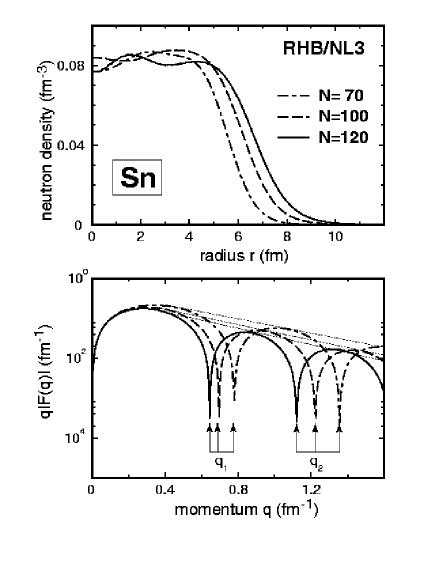
FIG. 1.: Top: neutron densities calculated in the RHB/NL3 model for ^120,150,170Sn. Bottom: the corresponding form factors. Positions of the first and second zeros in the form factors are indicated by arrows.

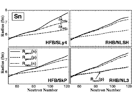
FIG. 2.: Neutron $R_{\rm geom}$(n) and $R_{\rm Helm}$(n), and proton $R_{\rm geom}$(p) radii for the Sn isotopes calculated in the HFB/SLy4, HFB/SkP, RHB/NLSH, and RHB/NL3 models. The proton Helm radius $R_{\rm Helm}$(p) is also shown in the RHB/NL3 variant (dotted line); it is very close to $R_{\rm geom}$(p).

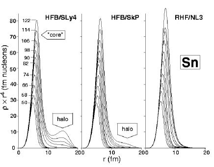
FIG. 3.: Neutron densities multiplied by $r^{4}$ for the tin isotopes with $N$=50, 28, 66, 74, 82, 90, 98, 106, 114, and 122 calculated in the HFB/SLy4, HFB/SkP, and RHB/NL3 models.

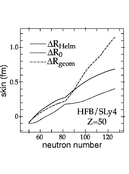
FIG. 4.: The neutron-proton radius differences (IV A) for the even-even Sn isotopes calculated in the HFB/SLy4 model.

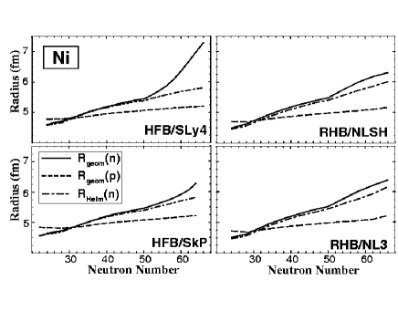
FIG. 5.: Same as in Fig. 2 except for the Ni isotopes.

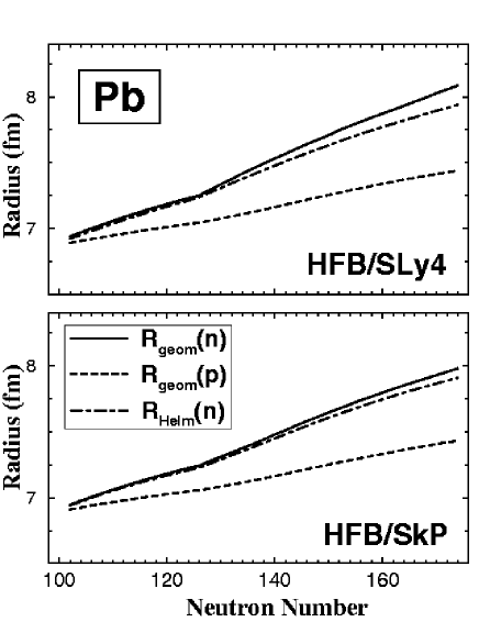
FIG. 6.: Neutron and proton radii for the Pb isotopes calculated in the HFB/SLy4 and HFB/SkP models.

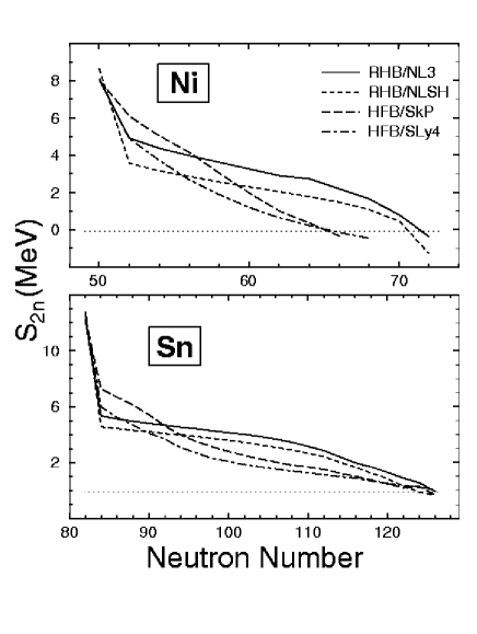
FIG. 7.: Two-neutron separation energies for the neutron-rich Ni (top) and Sn (bottom) isotopes calculated in the HFB/SLy4, HFB/SkP, RHB/NLSH, and RHB/NL3 models.

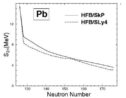
FIG. 8.: Two-neutron separation energies for the neutron-rich Pb isotopes calculated in the HFB/SLy4 and HFB/SkP models.

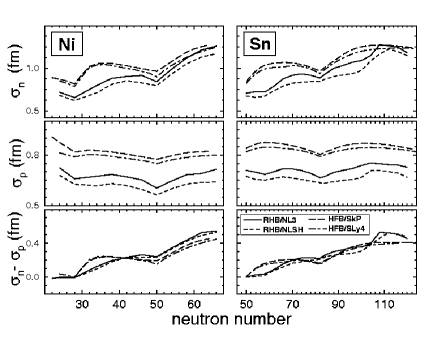
FIG. 9.: Neutron (top) and proton (middle) surface thickness coefficients for the Ni (left) and Sn (right) isotopes calculated in the RHB/NL3, RHB/NLSH, HFB/SkP, and HFB/SLy4 models. The difference, $\sigma_{n}$$-$$\sigma_{p}$, is shown in the bottom panels.

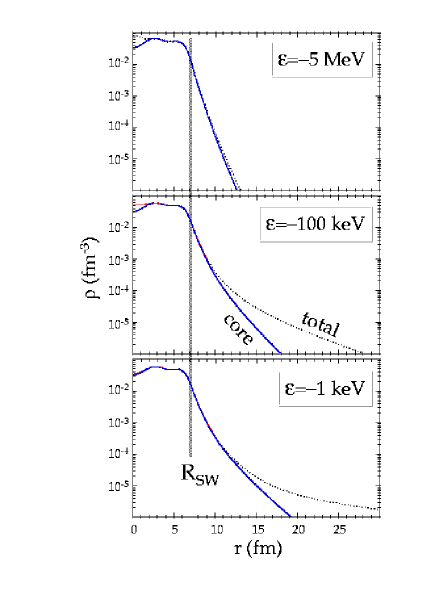
FIG. 10.: Total (dotted line) and core (solid line) densities for the system of 70 particles moving in the the finite spherical square-well potential with the radius $R_{\rm SW}$=7 fm for the three values of the binding energy of the $3s_{1/2}$ halo orbital: –5 MeV (top), –100 keV (middle), and –1 keV (bottom).

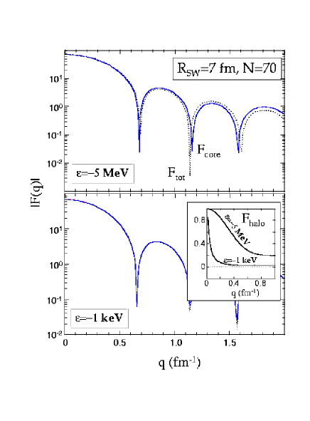
FIG. 11.: Form factors of the total (dotted line) and core (solid line) densities for the system of 70 particles moving in the finite spherical square-well potential with the radius $R_{\rm SW}$=7 fm for the two values of the binding energy of the $3s_{1/2}$ halo orbital: $-$5 MeV (top) and $-$1 keV (bottom). The form factor of the halo wave function is shown in the inset.

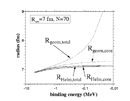
FIG. 12.: Dependence of the geometric radii, namely the total, $R_{\rm geom,total}$, and core, $R_{\rm geom,core}$ radii and of the corresponding Helm radii, $R_{\rm Helm,total}$ and $R_{\rm Helm,core}$, on the binding energy of the $3s_{1/2}$ halo orbital of the finite square well with radius $R_{\rm SW}$=7 fm. The total number of particles is $N$=70. The core consists of 68 particles occupying all the single-particle orbitals below $3s_{1/2}$.

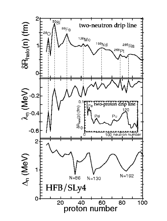
FIG. 13.: Neutron halo parameters (top), neutron Fermi energies (middle), and neutron pairing gaps (bottom) calculated in the HFB/SLy4 model for the two-neutron drip-line even-even nuclei (i.e., the heaviest even-even isotopes which are predicted to be two-neutron bound). The proton halo parameters for the two-proton drip-line even-even nuclei are shown in the inset. Note the correlation between $\delta R_{\rm halo}$ and $\lambda_{n}$, marked by the vertical dashed lines; whenever $\lambda_{n}$ approaches zero, $\delta R_{\rm halo}$ tends to increase.

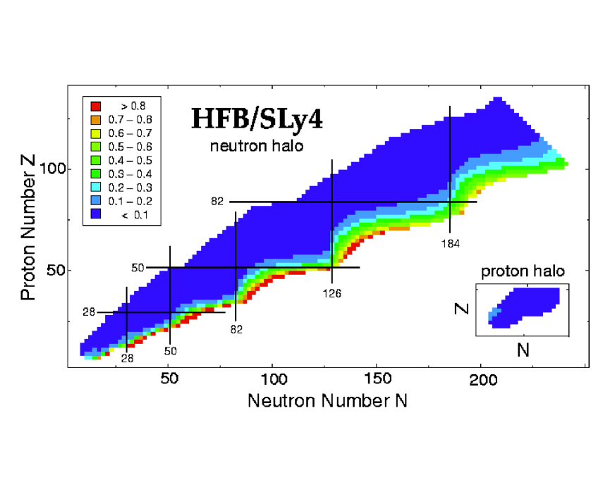
FIG. 14.: Neutron halo parameters (22) calculated in the spherical HFB/SLy4 model for two-particle stable even-even nuclei. The inset shows proton halo parameters for very light nuclei.

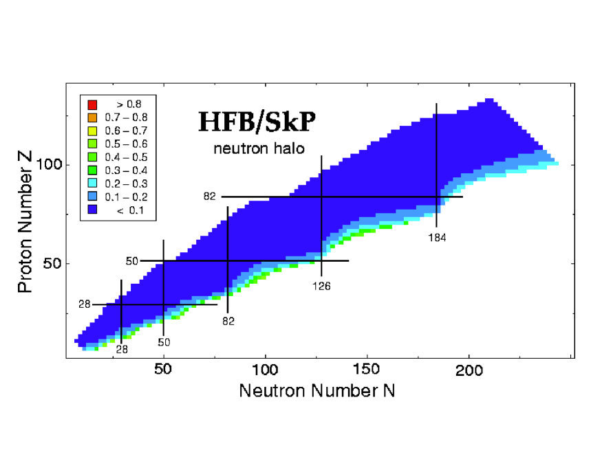
FIG. 15.: Neutron halo parameters (22) calculated in the spherical HFB/SkP model for two-particle stable even-even nuclei.

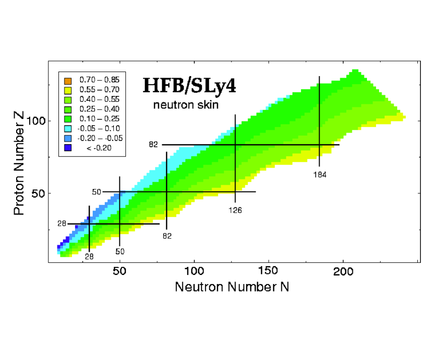
FIG. 16.: Skin parameters (29) calculated in the spherical HFB/SkP model for two-particle stable even-even nuclei.

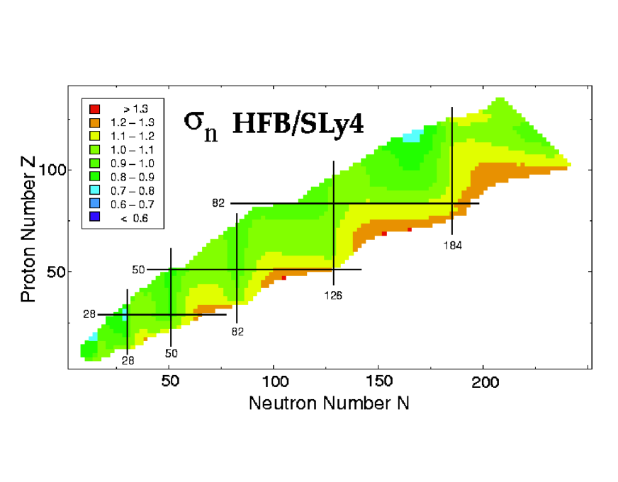
FIG. 17.: Neutron surface thickness calculated in the spherical HFB/SkP model for two-particle stable even-even nuclei.

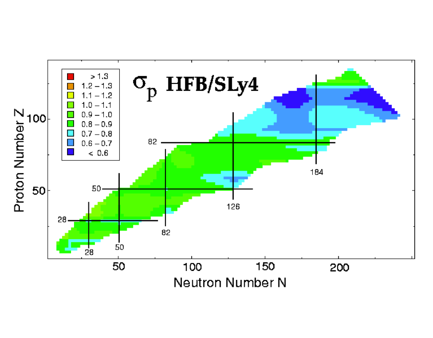
FIG. 18.: Same as in Fig. 17, except for the proton surface thickness.

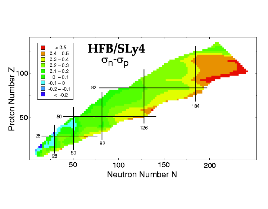
FIG. 19.: Same as in Fig. 17, except for the difference $\sigma_{n}-\sigma_{p}$.

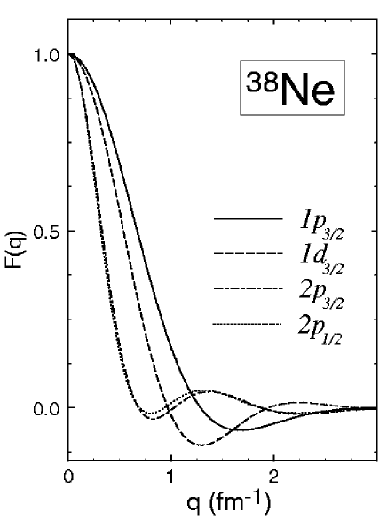
FIG. 20.: Form factors of canonical RHB/NL3 single-neutron orbitals 1$p_{3/2}$, 1$d_{3/2}$, 2$p_{3/2}$, and 2$p_{1/2}$ in ³⁸Ne.

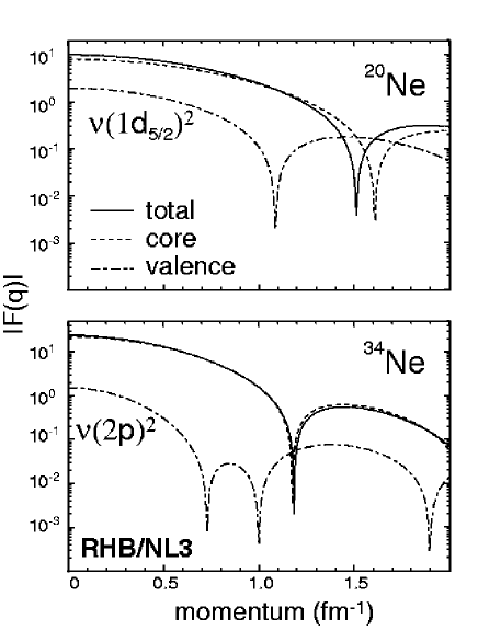
FIG. 21.: Total (solid line), core (dashed line), and valence (dash-dotted line) neutron form factors for ²⁰Ne (top) and ³⁴Ne (bottom). The valence space is here defined to be given by two $1d_{5/2}$ neutrons in ²⁰Ne and all the occupied $2p$ states in ³⁴Ne. The form factors at $q$=0 are normalized to the corresponding neutron numbers (e.g., $F_{\rm tot}(0)$=$N$).

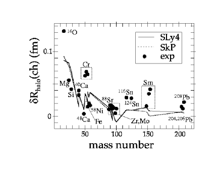
FIG. 22.: Comparison of experimental [98] and theoretical charge halos for a selection of stable nuclei. The spherical theoretical results are produced with the two Skyrme parametrizations SLy4 and SkP used throughout this paper. The estimated experimental errors are about 0.03 fm.