Abstract

We employ the chiral nucleon–nucleon potential derived in ref.[1] to study bound and scattering states in the two–nucleon system. At next–to–leading order, this potential is the sum of renormalized one–pion and two–pion exchange and contact interactions. At next–to–next–to-leading order, we have additional chiral two–pion exchange with low–energy constants determined from pion–nucleon scattering. Alternatively, we consider the $\Delta(1232)$ as an explicit degree of freedom in the effective field theory. The nine parameters related to the contact interactions can be determined by a fit to the $np$ S– and P–waves and the mixing parameter $\epsilon_{1}$ for laboratory energies below 100 MeV. The predicted phase shifts and mixing parameters for higher energies and higher angular momenta are mostly well described for energies below 300 MeV. The S–waves are described as precisely as in modern phenomenological potentials. We find a good description of the deuteron properties.

1 Introduction

Over the last years, effective field theory methods have been used to gain a better understanding of the two–nucleon interaction at low and intermediate energies. While at present these studies do not aim at substituting the highly successful “realistic” potentials build from meson exchanges (like the e.g. Bonn–Jülich, Nijmegen, Argonne or RuhrPot potential), effective field theory (EFT) allows for a systematic and controlled expansion of observables in systems with two or more nucleons. Apart from dealing with the various scales appearing in nuclear systems, it is straightforward to implement the spontaneously and explicitely broken chiral symmetry of QCD as well as external probes in the EFT. The appearance of shallow bound states (or, equivalently, large scattering lengths) requires some method of resummation. There are essentially two ways of tackling this problem. One approach is to build the potential from EFT and employ it in a properly regularized Lippmann–Schwinger (or Schrödinger) equation. Alternatively, one can also do the expansion directly on the level of the scattering amplitude and resum the leading order, momentum–independent four–nucleon interaction. While at extremely low energies, much below the scale set by the pion mass, it is sufficient to consider four–nucleon interactions only (otherwise the rather successfull effective range expansion would not work), for typical nuclear momenta of the size of the pion mass, pions have to be included explicitely. While there has been much debate about the way how to treat the pions (perturbative versus non–perturbative pions), for the range of momenta to be considered here we believe that it is mandatory to include them at leading order and treat them nonperturbatively. The results discussed below give an a posteriori justification of this conjecture. In fact, our chiral potential at next–to–next–to–leading order in the power counting leads to results which are only slightly worse than the ones based on the so–called high accuracy modern potentials.

In ref.[1] (referred to as I from here on) we constructed the two– and three–nucleon potential based on the most general chiral effective pion–nucleon Lagrangian using the method of unitary transformations. For that, we developed a power counting scheme consistent with this projection formalism. In contrast to previous results obtained in old–fashioned time–ordered perturbation theory, the method employed leads to energy–independent potentials. This extends the power counting scheme originally proposed by Weinberg [2] in a natural fashion. To leading order (LO), the potential consists of the undisputed one–pion exchange and two short–range four–fermion interactions. Corrections at next–to–leading order (NLO) stem from chiral two–pion exchange and additional contact terms with two derivatives. We extend the potential to next–to–next–to–leading order (NNLO) in two different ways. Apart from coupling constant and mass renormalization, one has only to consider the chiral two–pion–exchange potential (TPEP) with dimension two insertions from the pion–nucleon interaction. In contrast to ref.[3], we take the novel low–energy constants (LECs) from systematic studies of pion–nucleon scattering in CHPT [4, 5, 6, 7]. Alternatively, since most of these LECs are saturated by the $\Delta$–resonance, one can also include the $\Delta$ explicitely. That only introduces the $\pi N\Delta$ coupling as a new parameter. It can be determined e.g. from an (spin–isospin) SU(4) relation to the pion–nucleon coupling. In our approach the exchanges of heavy mesons (like in the CD-Bonn or Nijm93 potential) or parametrizations thereof (like in the AV18 or NijmI,II potential) show up as contact terms, but we refrain from a comparison of similarities and differences to the various potential model approaches at this point. A more detailed introduction of our method is given in I. Here, we will be concerned with numerical results obtained on the basis of that two–nucleon potential at NLO and NNLO. For that, we first have to renormalize the potential and discuss the appropriate cut–off regularization. Having done that, it is straightforward to solve the corresponding Lippmann–Schwinger equation for bound and scattering states. In total, we have nine parameters related to the four–fermion contact terms. These parameters can be uniquely fixed from fitting $np$ partial waves at low energies, more precisely the two S–, four P–waves and the mixing parameter $\epsilon_{1}$. Predictions for higher energies and the higher partial waves and deuteron properties arise (we refrain from fine tuning some of the parameters in the mixed ${}^{3}S_{1}-^{3}D_{1}$ waves to get the exact deuteron binding energy as it is done in conventional boson–exchange models).

To put our calculations in a better perspective, we briefly review the status of previous works (directly related to the results presented) without going into details. The idea of constructing the potential from effective field theory was put forward by Weinberg [2] in the early nineties. This was taken up by van Kolck and collaborators and culminated in ref.[3]. In that paper, the two–nucleon potential was constructed at next–next–to–leading order and analyzed. It contained one– and two–pion exchange graphs (based on time–ordered perturbation theory diagrams) and a host of contact interactions. An exponential cut–off at each vertex was introduced to tame the high energy behaviour. Fierz reordering was not used so that global fits with 26 parameters had to be performed and first numerical results for phase shifts and deuteron properties were obtained. While promising, these results were not as precise as the ones usually obtained in boson–exchange models. Park et al. [8] considered a series of interesting applications mostly related to the deuteron properties. They restricted themselves to one–pion–exchange and contact interactions for the relevant phases ${}^{1}S_{0},^{3}S_{1},^{3}D_{1}$ and the mixing parameter $\epsilon_{1}$. Peripheral nucleon–nucleon scattering was considered by the Munich group [9], including two–pion exchange graphs with insertions from the pion–nucleon Lagrangian of dimension two based on dimensionally regularized Feynman graphs. This lead to an improved description of some higher partial waves (for similar results, see the work of [10]). Since the potential was only considered perturbatively, the bound–state problem could not be addressed. A different counting scheme was proposed by Kaplan, Savage and Wise [11]. In that framework, the low partial waves and mixing parameters were considered to NLO and NNLO as well as many deuteron properties. A NNLO calculation of the ${}^{3}S_{1}-^{3}D_{1}$ transition potential matrix element was recently presented [12]. Further NNLO investigations for other partial waves in the framework of the KSW approach are under way by the Seattle group, see ref.[13].

Our manuscript is organized as follows. In sec.2, we explicitely give the renormalized potential at NLO and NNLO. This follows directly from the potential derived in I. We also discuss the regularization procedure necessecary to render the (iterated) potential finite. The Lippmann–Schwinger equation underlying the calculation of the scattering and bound states is briefly discussed in sec.3. The fitting procedure to determine the LECs and the accuracy of the fits are detailed in sec.4. This involves the low partial waves at (kinetic) energies (in the lab frame) below 100 MeV. Results for the low partial waves at higher energies, for the higher partial waves and the deuteron (bound state) properties are displayed and discussed in sec.5. Our findings are summarized in sec.6. The appendices contain details on the renormalization procedure, the inclusion of the $\Delta$–resonance and a collection of other useful formulas.

2 The renormalized potential

In I, we derived the two–nucleon potential at next–to–leading order. To leading order, it consists of the one–pion–exchange potential (which is called the OPEP) and two S–wave (non–derivative) contact interactions. The latter are parametrized by the coupling (low–energy) constants $C_{S}$ and $C_{T}$. The OPEP constitutes the longest range part of the nucleon–nucleon interaction and it completely dominates the high partial waves. However, the tensor potential related to one–pion–exchange becomes unrealistic at short distances. Chiral symmetry enforces a (pseudovector) derivative coupling in harmony with the Goldstone theorem. Note also that while the four–fermion interactions are pointlike on the level of the Lagrangian, they get smeared out by the regularization procedure to be discussed below. At next–to–leading order, we have three distinct contributions. The first ones are the one–loop self–energy and vertex corrections to the OPEP, cf. figs.3,4 in I. Similarly, it is mandatory to also work out the one–loop corrections to the contact terms $\sim C_{S},C_{T}$, cf. fig.6 in I. Thirdly, there are the genuine two–pion exchange diagrams, leading to the so–called TPEP, cf. fig.2 in I. This TPEP is the second longest range component of the $NN$ interaction. Here, chiral symmetry leads to the $\bar{N}N\pi\pi$ vertex which in turn leads to the so–called triangle and football diagrams. These are usually not accounted for in boson–exchange models. One notices immediately that some of the loop corrections contain UV divergences. Since we are dealing with an effective field theory, we can use the standard order–by–order renormalization machinery for the Lagrangian, which was first developed in the context of chiral perturbation theory. All these divergent contributions can be renormalized in terms of three divergent (momentum space) loop functions,

$$J_{0}=\int_{\varepsilon}^{\infty}\frac{dl}{l}~{},\quad J_{2}=\int_{0}^{\infty}l\,dl~{},\quad J_{4}=\int_{0}^{\infty}l^{3}\,dl~{}.$$ (2.1)

Clearly $J_{2}\,(J_{4})$ is quadratically (quartically) divergent while $J_{0}$ diverges logarithmically for large momenta and $\varepsilon$ is an IR regulator. Note that we could introduce other forms of the divergent integrals, which depend on one dimensionful scale (denoted here by $\varepsilon$). Another choice of defining this divergent loop integrals would give different finite subtractions but leads to the same non–polynomial terms in the potential. The precise renormalization procedure is discussed in app.A. Notice also that different to standard use, we perform the renormalization of the potential before regularizing the LS–equation as discussed below. Such an additional regularization is needed since loop as well as contact term contributions grow quadratically in momenta. More precisely, at NNLO some of the TPEP contributions even grow with the third power of momentum. Such an UV behaviour of the potential is, of course, unacceptable and requires additional regularization. The solutions of the LS–equation are adjusted to observables. Therefore, the renormalization constants are fixed and related to the regularization procedure in the LS–equation. This procedure is justified since the potential by itself is not an observable but rather the bound and scattering states obtained from the LS–equation. This should always be kept in mind.

We consider first the contact terms of the two–nucleon potential. To the accuracy we are working, the matrix–element of the potential in the center–of–mass system (cms) for initial and final nucleon momenta $\vec{p}$ and $\vec{p}~{}^{\prime}$, respectively, takes the form (note that due to the choice of the cms, a reduction in the number of terms follows as has been shown in I)

$$V^{{(\rm contact)}} = V^{(0)}+V^{(2)}~{},$$

$$V^{(0)} = C_{S}+C_{T}\,\vec{\sigma}_{1}\cdot\vec{\sigma}_{2}~{},$$

$$V^{(2)} = C_{1}\,\vec{q}\,^{2}+C_{2}\,\vec{k}^{2}+(C_{3}\,\vec{q}\,^{2}+C_{4}\,\vec{k}^{2})(\vec{\sigma}_{1}\cdot\vec{\sigma}_{2})+iC_{5}\,\frac{1}{2}\,(\vec{\sigma}_{1}+\vec{\sigma}_{2})\cdot(\vec{q}\times\vec{k})$$ (2.2)

$$+ C_{6}\,(\vec{q}\cdot\vec{\sigma}_{1})(\vec{q}\cdot\vec{\sigma}_{2})+C_{7}\,(\vec{k}\cdot\vec{\sigma}_{1})(\vec{k}\cdot\vec{\sigma}_{2})~{},$$

with $\vec{q}=\vec{p}~{}^{\prime}-\vec{p}$ and $\vec{k}=(\vec{p}+\vec{p}~{}^{\prime})/2$. These terms feed into the matrix–elements of the two S–waves (${}^{1}S_{0},^{3}S_{1}$), the four P–waves (${}^{1}P_{1},^{3}P_{1},^{3}P_{2},^{3}P_{0})$ and the lowest transition potential (${}^{3}D_{1}-^{3}S_{1}$) in the following way:

$$V(^{1}S_{0}) = {4\pi}\,(C_{S}-3C_{T})+\pi\,(4C_{1}+C_{2}-12C_{3}-3C_{4}-4C_{6}-C_{7})({p}^{2}+{p}^{\prime 2})~{},$$ (2.3)

$$= \tilde{C}_{{}^{1}S_{0}}+{C}_{{}^{1}S_{0}}({p}^{2}+{p}^{\prime 2})~{},$$

$$V(^{3}S_{1}) = {4\pi}\,(C_{S}+C_{T})+\frac{\pi}{3}\,(12C_{1}+3C_{2}+12C_{3}+3C_{4}+4C_{6}+C_{7})({p}^{2}+{p}^{\prime 2})~{},$$ (2.4)

$$= \tilde{C}_{{}^{3}S_{1}}+{C}_{{}^{3}S_{1}}({p}^{2}+{p}^{\prime 2})~{},$$

$$V(^{1}P_{1}) = \frac{2\pi}{3}\,(-4C_{1}+C_{2}+12C_{3}-3C_{4}+4C_{6}-C_{7})\,({p}\,{p}^{\prime})={C}_{{}^{1}P_{1}}\,({p}\,{p}^{\prime})~{},$$ (2.5)

$$V(^{3}P_{1}) = \frac{2\pi}{3}\,(-4C_{1}+C_{2}-4C_{3}+C_{4}+2C_{5}+4C_{6}+C_{7})\,({p}\,{p}^{\prime})={C}_{{}^{3}P_{1}}\,({p}\,{p}^{\prime})~{},$$

$$V(^{3}P_{2}) = \frac{2\pi}{3}\,(-4C_{1}+C_{2}-4C_{3}+C_{4}+2C_{5})\,({p}\,{p}^{\prime})={C}_{{}^{3}P_{2}}\,({p}\,{p}^{\prime})~{},$$ (2.7)

$$V(^{3}P_{0}) = \frac{2\pi}{3}\,(-4C_{1}+C_{2}-4C_{3}+C_{4}+4C_{5}+12C_{6}-3C_{7})\,({p}\,{p}^{\prime})={C}_{{}^{1}P_{0}}\,({p}\,{p}^{\prime})~{},$$

$$V(^{3}D_{1}-^{3}S_{1}) = \frac{2\sqrt{2}\pi}{3}\,(4C_{6}+C_{7})\,{p^{\prime}}^{2}={C}_{{}^{3}D_{1}-^{3}S_{1}}\,{p^{\prime}}^{2}~{},$$ (2.9)

$$V(^{3}S_{1}-^{3}D_{1}) = \frac{2\sqrt{2}\pi}{3}\,(4C_{6}+C_{7})\,{p}^{2}={C}_{{}^{3}D_{1}-^{3}S_{1}}\,{p}^{2}~{},$$ (2.10)

with $p=|\vec{p}\,|$ and ${p}^{\prime}=|\vec{p}\,^{\prime}|$. These nine constants are not fixed by chiral symmetry but can be determined by a fit to these lowest partial waves and one mixing parameter as detailed below. We have already given the appropriate partial wave decomposition for the low–energy constants (LECs) $C_{S},C_{T},C_{1},\ldots,C_{7}$ here. From each of the two S–waves, we can determine two parameters, whereas the four P–waves and the mixing parameter $\epsilon_{1}$ contain one free parameter each. Of course, we have to account for the channel coupling in the mixed triplet partial waves. It is also important to note that once the $C_{{}^{2s+1}l_{j}}$ have been determined, the original $C_{S},C_{T},C_{1},\ldots,C_{7}$ are fixed uniquely. We remark that the values for the $C_{{}^{2s+1}l_{j}}$ are renormalized quantities, see app.A.

Consider now OPEP and TPEP. After vertex and coupling constant renormalization, as detailed in app.A, we find the following expressions in terms of the renormalized quantities at NLO:

$$V^{\rm OPEP} = -\biggl{(}\frac{g_{A}}{2f_{\pi}}\biggr{)}^{2}\,\vec{\tau}_{1}\cdot\vec{\tau}_{2}\,\frac{\vec{\sigma}_{1}\cdot\vec{q}\,\vec{\sigma}_{2}\cdot\vec{q}}{q^{2}+M_{\pi}^{2}}~{},$$ (2.11)

$$V^{\rm TPEP}_{\rm NLO} = -\frac{\vec{\tau}_{1}\cdot\vec{\tau}_{2}}{384\pi^{2}f_{\pi}^{4}}\,L(q)\,\biggl{\{}4M_{\pi}^{2}(5g_{A}^{4}-4g_{A}^{2}-1)+q^{2}(23g_{A}^{4}-10g_{A}^{2}-1)+\frac{48g_{A}^{4}M_{\pi}^{4}}{4M_{\pi}^{2}+q^{2}}\biggr{\}}$$ (2.12)

$$-\frac{3g_{A}^{4}}{64\pi^{2}f_{\pi}^{4}}\,L(q)\,\biggl{\{}\vec{\sigma}_{1}\cdot\vec{q}\,\vec{\sigma}_{2}\cdot\vec{q}-q^{2}\,\vec{\sigma}_{1}\cdot\vec{\sigma}_{2}\biggr{\}}+P(\vec{k},\vec{q}\,)~{},$$

with

$$L(q)=\frac{1}{q}\sqrt{4M_{\pi}^{2}+q^{2}}\,\ln\frac{\sqrt{4M_{\pi}^{2}+q^{2}}+q}{2M_{\pi}}~{},$$ (2.13)

and we have set $q\equiv|\vec{q}\,|$. Furthermore, $f_{\pi}=93\,$MeV is the pion decay constant, $M_{\pi}=138.03\,$MeV the pion mass and $g_{A}=1.26$ for the axial–vector coupling. Furthermore, $P(\vec{k},\vec{q}\,)$ is a polynom in momenta of at most second degree and has the same structure as the expressions in eq.(2). More precisely, after performing the partial decomposition, $P(\vec{k},\vec{q}\,)$ leads in each partial wave to polynoms in $\vec{p}$ and $\vec{p}\,^{\prime}$ of at most second degree. Thus, its explicit form is of no relevance here, since it only contributes to the renormalization of the couplings $C_{S},C_{T},C_{i}$, as detailed in app.A. The TPEP agrees with the one given by the Munich group. It is important to stress the differences to the calculation of ref.[9]. While there the potential was treated perturbatively, we iterate it to all orders in a Lippmann–Schwinger (LS) equation. Second, we use a cut–off regularization within the LS–equation and not dimensional regularization on the level of the diagrams. Of course, for the peripheral partial waves, the iteration is not of importance. We are, however, more ambitious in that we want to get a description of all partial waves as well as of the bound state (deuteron) properties. The TPEP at NNLO has also been given in ref.[9] using dimensional regularization. Within our renormalization scheme, it reads:

$$V^{\rm TPEP}_{\rm NNLO} = -\frac{3g_{A}^{2}}{16\pi f_{\pi}^{4}}\biggl{\{}-\frac{g_{A}^{2}M_{\pi}^{5}}{16m(4M_{\pi}^{2}+q^{2})}+\biggl{(}2M_{\pi}^{2}(2c_{1}-c_{3})-q^{2}\,\bigl{(}c_{3}+\frac{3g_{A}^{2}}{16m}\bigr{)}\biggr{)}(2M_{\pi}^{2}+q^{2})A(q)\biggr{\}}$$ (2.14)

$$- \frac{g_{A}^{2}}{128\pi mf_{\pi}^{4}}(\vec{\tau}_{1}\cdot\vec{\tau}_{2})\,\biggl{\{}-\frac{3g_{A}^{2}M_{\pi}^{5}}{4M_{\pi}^{2}+q^{2}}+\bigl{(}4M_{\pi}^{2}+2q^{2}-g_{A}^{2}(4M_{\pi}^{2}+3q^{2})\bigr{)}(2M_{\pi}^{2}+q^{2})A(q)\biggr{\}}$$

$$+ \frac{9g_{A}^{4}}{512\pi mf_{\pi}^{4}}\biggl{(}(\vec{\sigma}_{1}\cdot\vec{q}\,)(\vec{\sigma}_{2}\cdot\vec{q}\,)-q^{2}(\vec{\sigma}_{1}\cdot\vec{\sigma}_{2})\biggr{)}\,(2M_{\pi}^{2}+q^{2})A(q)$$

$$- \frac{g_{A}^{2}}{32\pi f_{\pi}^{4}}(\vec{\tau}_{1}\cdot\vec{\tau}_{2})\,\biggl{(}(\vec{\sigma}_{1}\cdot\vec{q}\,)(\vec{\sigma}_{2}\cdot\vec{q}\,)-q^{2}(\vec{\sigma}_{1}\cdot\vec{\sigma}_{2})\biggr{)}$$

$$\qquad\qquad\qquad\qquad\qquad\qquad\times\biggl{\{}\bigl{(}c_{4}+\frac{1}{4m}\bigr{)}(4M_{\pi}^{2}+q^{2})-\frac{g_{A}^{2}}{8m}(10M_{\pi}^{2}+3q^{2})\biggr{\}}\,A(q)$$

$$- \frac{3g_{A}^{4}}{64\pi mf_{\pi}^{4}}\,i\,(\vec{\sigma}_{1}+\vec{\sigma}_{2})\cdot(\vec{p}~{}^{\prime}\times\vec{p})\,(2M_{\pi}^{2}+q^{2})A(q)$$

$$- \frac{g_{A}^{2}(1-g_{A}^{2})}{64\pi mf_{\pi}^{4}}(\vec{\tau}_{1}\cdot\vec{\tau}_{2})\,i\,(\vec{\sigma}_{1}+\vec{\sigma}_{2})\cdot(\vec{p}~{}^{\prime}\times\vec{p})\,(4M_{\pi}^{2}+q^{2})A(q)+\tilde{P}(\vec{k},\vec{q}\,)~{},$$

with

$$A(q)=\frac{1}{2q}\arctan\frac{q}{2M_{\pi}}~{}.$$ (2.15)

The polynom $\tilde{P}(\vec{k},\vec{q}\,)$ plays a similar role as $P(\vec{k},\vec{q}\,)$ in eq.(2.12). Note that we have used the standard dimension two $\pi N$ Lagrangian as in ref.[9]. For the LECs $c_{1,3,4}$ we should take the values obtained from fitting $\pi N$ phases in the threshold region, see e.g. ref.[6] or, alternatively, from fitting the invariant amplitudes inside the Mandelstam triangle, i.e. in the unphysical region [7]. The so determined parameters are only slightly different, but these small differences will play a role later on. For example, the LECs $c_{1,3,4}$ from fit 1 of ref.[6] are $c_{1}=-1.23\,$GeV^-1, $c_{3}=-5.94\,$GeV^-1 and $c_{4}=3.47\,$GeV^-1. A recent investigation of the subthreshold amplitudes [7] leads to slightly different values, $c_{1}=-0.81\,$GeV^-1, $c_{3}=-4.70\,$GeV^-1 and $c_{4}=3.40\,$GeV^-1. It is this latter set we will use in the following. These values are also consistent with the recent determination from the proton–proton interaction based on the chiral two–pion exchange potential [14].

The total renormalized potential at NLO is now given as the sum of the OPEP, TPEP and contact potentials as given in eqs.(2.11,2.12,2). At NNLO, we have to add the additional TPEP from eq.(2.14). Alternatively, we have also included the leading contribution from the $\Delta(1232)$ resonance. This is formally a NNLO contribution as demanded by the decoupling theorem. The pertinent equations are collected in app. B. We only remark that there is one new parameter, namely the $\Delta N\pi$ coupling constant. It can be determined from the SU(4) relation

$$g_{\Delta N\pi}=\frac{3}{\sqrt{2}}\,\frac{g_{A}\,m}{F_{\pi}}~{},$$ (2.16)

making use of the Goldberger–Treiman relation (GTR) (higher order corrections to the GTR are not considered here). This leads to $g_{\Delta N\pi}=27.2$, as detailed in app. B. The corresponding theory is called NNLO–$\Delta$. The chiral TPEP has a different high momentum behaviour as in the strict NNLO approach because of the explicit $\Delta$–propagator (assuming that we only include the $\Delta$ to generate the NNLO TPEP and no additional $\pi N$ contact interactions). Only for small momenta NNLO and NNLO–$\Delta$ are essentially the same (resonance saturation). At this point, we already mention that the NNLO TPEP is too strong at short distances (large momenta). To the order we are working, we have counterterms in the S– and P–waves to balance this, but e.g. not in the D–waves. This will be discussed in more details below.

Since the potential is only meaningful for momenta below a certain scale, it needs regularization. Stated differently, the large momentum behaviour of the potential is not correct. To the order we are working, the contact interactions diverge quadratically for large momenta and some components of the TPEP grow even with the third power of momentum. As it is appropriate in effective field theory, we regularize the potential. That is done in the following way:

$$V(\vec{p},\vec{p}~{}^{\prime}\,)\to f_{R}(\vec{p}\,)\,V(\vec{p},\vec{p}~{}^{\prime}\,)\,f_{R}(\vec{p}~{}^{\prime}\,)~{},$$ (2.17)

where $f_{R}(\vec{p}\,)$ is a regulator function chosen in harmony with the underlying symmetries. In what follows, we work with two different regulator functions,

$$f_{R}^{\rm sharp}(\vec{p}\,) = \theta(\Lambda^{2}-p^{2})~{},$$ (2.18)

$$f_{R}^{\rm expon}(\vec{p}\,) = \exp(-p^{2n}/\Lambda^{2n})~{},$$ (2.19)

with $n=2,3,\ldots\,$. The sharp cut–off is most appropriate to the projection formalism. For the calculation of some observables, however, it cannot be used since at $p,p^{\prime}=\Lambda$ it leads to discontinous derivatives. For very large integers $n$ the exponential cut–off approximates the sharp one. Throughout, we work with $n=2$. To the order we are working, the choice $n=1$ has to be excluded since the contact terms of order $p^{2},{p^{\prime}}^{2}$ would be modified. For $n=2$, the error we make is beyond the accuracy of the order we are calculating. We are now in the position to calculate observables with this potential.

3 Bound and scattering state equation

In ref.[3], the Schrödinger equation was solved after the chiral NN potential had been transformed from momentum into co-ordinate space. We consider it more natural to work directly in momentum space. The corresponding equation describing the bound and scattering states is the Lippmann–Schwinger equation. Here, we briefly discuss it to keep the manuscript self–contained. For a more detailed exposition concerning also methods of solving the LS–equation, we refer to the monograph [15].

The LS–equation (for the T–matrix) projected into states with orbital angular momentum $l$, total spin $s$ and total angular momentum $j$ is

$$T^{sj}_{l^{\prime},l}(p^{\prime},p)=V^{sj}_{l^{\prime},l}(p^{\prime},p)+\sum_{l^{\prime\prime}}\,\int_{0}^{\infty}\frac{dp^{\prime\prime}\,{p^{\prime\prime}}^{2}}{(2\pi)^{3}}\,V^{sj}_{l^{\prime},l^{\prime\prime}}(p^{\prime},p^{\prime\prime})\frac{1}{p^{2}-{p^{\prime\prime}}^{2}-i\eta}T^{sj}_{l^{\prime\prime},l}(p^{\prime\prime},p)~{},$$ (3.1)

with $\eta\to 0^{+}$. In the uncoupled case, $l$ is conserved. The partial wave projected potential $V^{sj}_{l^{\prime},l}(p^{\prime},p)$ is obtained as follows. We first rewrite the potential $V$ in the form [16]

$$V = V_{C}+V_{\sigma}\;\vec{\sigma}_{1}\cdot\vec{\sigma}_{2}+V_{SL}\;i\;\frac{1}{2}(\vec{\sigma}_{1}+\vec{\sigma}_{2})\cdot(\vec{k}\times\vec{q})+V_{\sigma L}\;\vec{\sigma}_{1}\cdot(\vec{q}\times\vec{k})\;\vec{\sigma}_{2}\cdot(\vec{q}\times\vec{k})$$ (3.2)

$${}+V_{\sigma q}\;(\vec{\sigma}_{1}\cdot\vec{q})\;(\vec{\sigma}_{2}\cdot\vec{q})+V_{\sigma k}\;(\vec{\sigma}_{1}\cdot\vec{k})\;(\vec{\sigma}_{2}\cdot\vec{k})$$

with six functions $V_{C}(p,p^{\prime},z),\;\ldots,\;V_{\sigma k}(p,p^{\prime},z)$ depending on $p\equiv|\vec{p}\,|$, $p^{\prime}\equiv|\vec{p}\,^{\prime}|$ and the cosine of the angle between the two momenta $z$. These functions may depend on the isospin matrices $\vec{\tau}$ as well. For $j>0$, one obtains in the usual $lsj$ representation

$$\langle j0j|V|j0j\rangle = 2\pi\int_{-1}^{1}\,dz\,\left\{V_{C}-3V_{\sigma}+{p^{\prime}}^{2}{p}^{2}(z^{2}-1)V_{\sigma L}-q^{2}V_{\sigma q}-k^{2}V_{\sigma k}\right\}P_{j}(z)~{},$$

$$\langle j1j|V|j1j\rangle = 2\pi\int_{-1}^{1}\,dz\,\left\{\left[V_{C}+V_{\sigma}+2p^{\prime}pzV_{SL}-{p^{\prime}}^{2}p^{2}(1+3z^{2})V_{\sigma L}+4k^{2}V_{\sigma q}+\frac{1}{4}q^{2}V_{\sigma k}\right]\right.$$

$${}\times P_{j}(z)+\left.\left[-p^{\prime}p\,V_{SL}+2{p^{\prime}}^{2}p^{2}zV_{\sigma L}-2p^{\prime}p\,(V_{\sigma q}-\frac{1}{4}V_{\sigma k})\right]\right.$$

$${}\times\left(P_{j-1}(z)+P_{j+1}(z)\right)\bigg{\}}~{},$$

$$\langle j\pm 1,1j|V|j\pm 1,1j\rangle = 2\pi\int_{-1}^{1}\,dz\,\left\{p^{\prime}p\left[-V_{SL}\pm\frac{2}{2j+1}\left(-p^{\prime}pzV_{\sigma L}+V_{\sigma q}-\frac{1}{4}V_{\sigma k}\right)\right]\right.$$

$${}\times P_{j}(z)+\bigg{[}V_{C}+V_{\sigma}+p^{\prime}pzV_{SL}+{p^{\prime}}^{2}p^{2}(1-z^{2})V_{\sigma L}$$

$${}\left.\left.\pm\frac{1}{2j+1}\left(2{p^{\prime}}^{2}p^{2}V_{\sigma L}-({p^{\prime}}^{2}+p^{2})(V_{\sigma q}+\frac{1}{4}V_{\sigma k})\right)\right]P_{j\pm 1}(z)\right\}$$

$$\langle j\pm 1,1j|V|j\mp 1,1j\rangle = \frac{\sqrt{j(j+1)}}{2j+1}2\pi\int_{-1}^{1}\,dz\,\Bigg{\{}-p^{\prime}p\,(4V_{\sigma q}-V_{\sigma k})P_{j}(z)~{},$$

$${}+\left[\mp\frac{2{p^{\prime}}^{2}p^{2}}{2j+1}V_{\sigma L}+{p^{\prime}}^{2}\Big{(}2V_{\sigma q}+\frac{1}{2}V_{\sigma k}\Big{)}\right]P_{j\mp 1}(z)$$

$${}\left.+\left[\pm\frac{2{p^{\prime}}^{2}p^{2}}{2j+1}V_{\sigma L}+{p}^{2}\Big{(}2V_{\sigma q}+\frac{1}{2}V_{\sigma k}\Big{)}\right]P_{j\pm 1}(z)\right\}~{}.$$

Here, $P_{j}(z)$ are the conventional Legendre polynomials. For $j=0$ the two nonvanishing matrix elements are

$$\langle 000|V|000\rangle = 2\pi\int_{-1}^{1}\,dz\,\left\{V_{C}-3V_{\sigma}+{p^{\prime}}^{2}{p}^{2}(z^{2}-1)V_{\sigma L}-q^{2}V_{\sigma q}-k^{2}V_{\sigma k}\right\}~{},$$

$$\langle 110|V|110\rangle = 2\pi\int_{-1}^{1}\,dz\,\bigg{\{}zV_{C}+zV_{\sigma}+p^{\prime}p(z^{2}-1)V_{SL}+{p^{\prime}}^{2}p^{2}z(1-z^{2})V_{\sigma L}$$

$${}\left.-\left(({p^{\prime}}^{2}+p^{2})z-2p^{\prime}p\right)V_{\sigma q}-\frac{1}{4}\left(({p^{\prime}}^{2}+p^{2})z+2p^{\prime}p\right)V_{\sigma k}\right\}~{}.$$

Note that sometimes another notation is used in which an additional overall “-” sign enters the expressions for the off–diagonal matrix elements with $l=j+1,\,l^{\prime}=j-1$ and $l=j-1,\,l^{\prime}=j+1$.

The relation between the on–shell $S$– and $T$–matrices is given by

$$S_{l^{\prime}l}^{sj}(p)=\delta_{l^{\prime}l}-\frac{i}{8\pi^{2}}\,p\,m\,T_{l^{\prime}l}^{sj}(p)~{},$$ (3.5)

where $p$ denotes the two–nucleon center–of–mass three–momentum. The phase shifts in the uncoupled cases can be obtained from the $S$–matrix via

$$S_{jj}^{0j}=\exp{\left(2i\delta_{j}^{0j}\right)}\;,\quad S_{jj}^{1j}=\exp{\left(2i\delta_{j}^{1j}\right)}\;,$$ (3.6)

where we have used the notation $\delta^{sj}_{l}$. Throughout, we use the so–called Stapp parametrization [17] of the $S$–matrix in the coupled channels ($j>0$):

$$S=\left(\begin{array}[]{cc}S_{j-1\,j-1}^{1j}&S_{j-1\,j+1}^{1j}\\ S_{j+1\,j-1}^{1j}&S_{j+1\,j+1}^{1j}\end{array}\right)=\left(\begin{array}[]{cc}\cos{(2\epsilon)}\exp{(2i\delta^{1j}_{j-1})}&i\sin{(2\epsilon)}\exp{(i\delta^{1j}_{j-1}+i\delta^{1j}_{j+1})}\\ i\sin{(2\epsilon)}\exp{(i\delta^{1j}_{j-1}+i\delta^{1j}_{j+1})}&\cos{(2\epsilon)}\exp{(2i\delta^{1j}_{j+1})}\end{array}\right)~{}.$$ (3.7)

The bound state is obtained from the homogeneous part of eq.(3.1) and obeys

$$\phi_{l}(p)=\frac{1}{E_{d}-p^{2}/m}\,\sum_{l^{\prime}}\,\int_{0}^{\infty}\frac{dp^{\prime}\,{p^{\prime}}^{2}}{(2\pi)^{3}}\,V^{sj}_{l,l^{\prime}}(p,p^{\prime})\,\phi_{l^{\prime}}(p^{\prime})~{},$$ (3.8)

with $s=j=1$ and $l=l^{\prime}=0,2$ and $E_{d}$ denotes the bound–state energy. The LS-equations for the scattering and the bound state(s) are solved by standard Gauss–Legendre quadrature. It goes without saying that in this discussion, the potential is to be understood in its regularized form as detailed in eqs.(2.17, 2.18, 2.19).

4 The fits

In this section we discuss the determination of the various coupling constants. The leading OPEP is constrained by chiral symmetry, its strength is given by the pion–nucleon coupling constant, which due to the Goldberger–Treiman relation is proportional to $g_{A}/f_{\pi}$. For the NNLO–$\Delta$ approach, we in addition have the strong pion–nucleon–$\Delta$ coupling constant.

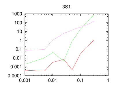
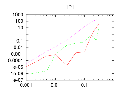
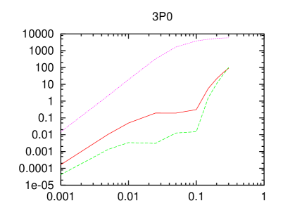
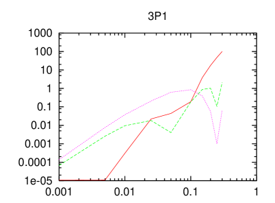
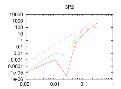
Figure 1: Quadratic deviations in the phase shifts, $(\delta^{\rm fit}-\delta^{\rm PSA})^{2}$, versus $E_{\rm lab}$ in GeV. Data from the Nijmegen PSA have been fitted for $E_{\rm lab}\leq 0.1\,$ GeV. The purple dotted, green dashed and red solid curves represent LO, NLO and NNLO results, respectively.

To pin down the nine parameters $C_{S},C_{T},C_{1},\ldots,C_{7}$ we do not perform global fits as done in ref.[3]. Rather we introduce the independent new parameters as given in eqs.(2.3–2.10). So to leading order, the two S– waves are depending on one parameter each. At NLO, we have one additional parameter for ${}^{1}S_{0}$ and ${}^{3}S_{1}$ as well as one parameters in each of the four P–waves and in $\epsilon_{1}$. We thus can fit each partial wave separately, which makes the fitting procedure not only extremely simple but also unique. Of course, in case of the triplet coupled waves (${}^{3}S_{1}-^{3}D_{1},^{3}P_{2}-^{3}F_{2})$ the fitting is performed for the corresponding $2\times 2$ S–matrix parametrizations (parametrized by two partial waves and one mixing parameter). At NNLO (NNLO–$\Delta$), we have no new parameters, but must refit the various contact interactions due to the TPEP contribution in all partial waves. We have used two different methods to fix the LECs of the contact interactions. First, we fit to the phase shifts of the Nijmegen partial wave analysis [22] for laboratory energies smaller than (50) 100 MeV at (NLO) NNLO. Alternatively, we used the effective range parameters for the phases ${}^{1}S_{0}$, ${}^{3}S_{1}$ and $\epsilon_{1}$ to fix $\tilde{C}_{{}^{1}S_{0}},{C}_{{}^{1}S_{0}},\tilde{C}_{{}^{3}S_{1}},{C}_{{}^{3}S_{1}},$ and ${C}_{{}^{3}D_{1}-^{3}S_{1}}$. In what follows we will mark the corresponding potentials by a “$\star$” if the LECs were fixed from the effective range parameters. We have found that the observables (phase shifts) depend rather weekly on what fitting procedure is used. The values of the LECs do not change much except for some $C$’s at NLO, where significant variations were observed. Note further that in the S–waves, especially in ${}^{1}S_{0}$, isospin breaking effects like e.g. the charged to neutral pion mass difference, are known to be important. We do not consider such effects in this work and thus take an average value for the pion mass. The actual values of the S–wave LECs seem to be rather sensitive to the choice of the pion mass. For the phases ${}^{1}S_{0}$, ${}^{3}S_{1}$ and $\epsilon_{1}$ we use the errors as given in ref.[22], for all other partial waves we assign an absolute error of 3%. This number is arbitrary, but taking any other value would not change the fit results, only the total $\chi^{2}$. To perform the fits, we have to specify the value of the cut–off $\Lambda$ in the regulator functions as defined in eqs.(2.18,2.19). At NLO, for any choice between 380 MeV and 600 MeV, we get very similar fits (a very shallow $\chi^{2}$ distribution in each partial wave). At NNLO, this shallow distribution turns into a plateau, which shifts to higher values of the cut–off. We can now use values between 600 MeV and 1 GeV. The results using the sharp or the exponential cut–off are very similar. For illustration, we consider the sharp cut–off with $\Lambda=500\,$MeV at NLO and $\Lambda=875\,$MeV at NNLO. We show in fig. 1 the absolute quadratic deviations of the fit to the Nijmegen phase shift analysis (PSA), defined by $(\delta^{\rm fit}-\delta^{\rm PSA})^{2}$. Consider first the S–waves. Both in ${}^{1}S_{0}$ and ${}^{3}S_{1}$, we observe a clear improvement when going from LO to NLO to NNLO (NNLO–$\Delta$). A similar pattern holds for the P–waves and $\epsilon_{1}$, although the differences between NLO and NNLO are somewhat less pronounced. Note that the ${}^{3}P_{0}$ wave is very senstive to the value of the pion mass, therefore the slightly better NLO fit should not be considered problematic. The corresponding parameters of the coupling constants are collected in table 1.

	$\tilde{C}_{{}^{1}S_{0}}$	${C}_{{}^{1}S_{0}}$	$\tilde{C}_{{}^{3}S_{1}}$	${C}_{{}^{3}S_{1}}$	$C_{{}^{1}P_{1}}$	$C_{{}^{3}P_{1}}$	$C_{{}^{3}P_{0}}$	$C_{{}^{3}P_{2}}$	$C_{{}^{3}D_{1}-^{3}S_{1}}$
NLO	$-$0.134	1.822	$-$0.130	$-$0.393	0.344	$-$0.394	1.335	$-$0.1907	$-$0.0317
NLO$\star$	$-$0.0928	2.125	$-$0.102	0.0243	0.344	$-$0.394	1.335	$-$0.191	$-$0.0357
NNLO	$-$4.249	11.945	$-$6.508	11.293	$-$2.045	$-$7.061	$-$2.832	$-$8.056	$-$3.424
NNLO$\star$	$-$4.246	11.943	$-$6.655	11.279	$-$2.045	$-$7.061	$-$2.832	$-$8.056	$-$3.516
NNLO-$\Delta$	$-$5.731	13.823	$-$0.977	3.446	$-$2.494	$-$8.188	$-$2.993	$-$8.431	$-$0.562

Table 1: The values of the LECs as determined from the low partial waves. We use a sharp cut–off with $\Lambda=500$ MeV and 875 MeV at NLO and NNLO, respectively. The $\tilde{C}_{i}$ are in $10^{4}$ GeV^-2 while the others are in $10^{4}$ GeV^-4. The parameters of the NLO, NNLO and NNLO–$\Delta$ potentials are obtained from fitting to the Nijmegen PSA. The LECs of the NLO$\star$, NNLO$\star$ potential in the ${}^{1}S_{0}$ and ${}^{3}S_{1}-^{3}D_{1}$ channels are fixed to reproduce exactly the effective range parameters.

To illustrate the dependence on the cut–off, we show in fig.2 the running of the two (three) couplings in the ${}^{1}S_{0}$ (${}^{3}S_{1}$) channels at NNLO (note that the third parameter in ${}^{3}S_{1}$ comes in via the mixing with the ${}^{3}D_{1}$ wave). We notice that the variation of these LECs over a wide range of cut–offs is rather modest. We also mention that using the $\pi N$ parameters from refs.[4, 5, 6] leads to a considerably worse $\chi^{2}$ in the fits. We take that as an indication that the determination of the $c_{i}$ based on the method employed in ref.[7] is more reliable than fitting to $\pi N$ phase shifts (as long as one works to third order in the chiral expansion). We remark that using the parameters of ref.[7], the deuteron binding energy $E_{d}$ comes out as

$${\rm NLO} : E_{d}=-2.175\,{\rm MeV}~{},$$

$${\rm NNLO} : E_{d}=-2.208\,{\rm MeV}~{},$$ (4.1)

i.e. the NNLO result is already within 7.5 permille of the experimental number. Fine tuning in the parameters in the deuteron channel would allow to get the binding energy at the exact value of $-2.224575(9)\,$MeV without leading to any noticeable change in the phase shifts. We later consider the deuteron channel separately with an exponential regulator. This will lead to an improved binding energy but no attempt is made to match the exact value in all digits.

At this point we would like to comment on the increase in the cut–off values when going from NLO to NNLO (NNLO–$\Delta$). Consider first the leading order result. Lepage [23] has pointed out that inclusion of the one–pion exchange does not lead to a remarkable increase in the cut–off values compared to a pionless theory. In order to fit the phase shifts in the S–waves one should choose the cut–off below 500–600 MeV even if the contact interactions with two derivatives are taken into account (within our power counting scheme such contact interactions contribute first at next–to–leading order and are of the same size as the lading two–pion exchange terms). Lepage assumed that such a low value of the cut–off is due to the missed physics assosiated with the two–pion exchange. So, naively, one would expect that the inclusion of the leading two–pion exchange contributions at NLO would allow to take larger cut–off values. However, that does not happen. This was also pointed out in ref.[24]. According to our analysis only at NNLO, after the subleading two–pion exchange contributions are taken into account, one can increase the cut–off up to 800 to 1000 MeV. The inclusion of the dimension two operators of the pion–nucleon interaction at NNLO encodes some information about heavy meson exchange as well as virtual isobar excitations, as discussed in detail in ref.[4]. In this work we were able to separate the leading effects of $\Delta$–resonance (NNLO–$\Delta$). The clear increase in the cut–off values when going from NLO to NNLO–$\Delta$ indicates the importance of physics assosiated with heavier mass states like e.g. the $\Delta$-resonance. Our NNLO (NNLO–$\Delta$) TPEP is sensitive to momentum scales sizeably larger than twice the pion mass (as it would be the case for uncorrelated TPE) and delta–nucleon mass splitting. Consequently, the cut–off has to be chosen safely above these scales, say above 500 MeV (with the sharp regulator). The upper limit of about 1 GeV is related to the cancellations in the S–waves (fine–tuning), for too large values of $\Lambda$ it is not longer possible to keep this intricate balance. It is, however, comforting to see that including more physics in the potential leads indeed to a wider range of applicability of the EFT.

Finally, we need to discuss one further topic. Performing the fits, we have found two minima in both the ${}^{1}S_{0}$ and the ${}^{3}S_{1}$ channel. This is not unexpected and can easily be understood in the case of a pionless theory. In that case, exact analytical calculations are possible. As was shown in ref.[25], the requirement of reproducing exactly the scattering length and the effective range leads to the following conditions for the LECs in the ${}^{1}S_{0}$ partial wave,

$$\frac{m}{16\pi^{2}a} = \frac{(C_{{}^{1}S_{0}}I_{3}-1)^{2}}{\tilde{C}_{{}^{1}S_{0}}+C_{{}^{1}S_{0}}^{2}I_{5}}-I_{1}\quad,$$

$$\frac{mr}{32\pi^{2}} = \biggl{(}\frac{m}{16\pi^{2}a}+I_{1}\biggr{)}^{2}\,\frac{C_{{}^{1}S_{0}}(2-C_{{}^{1}S_{0}}I_{3})}{(C_{{}^{1}S_{0}}I_{3}-1)^{2}}+\frac{m}{(2\pi)^{3}\Lambda}~{},$$ (4.2)

where

$$I_{n}=-m\int_{0}^{\Lambda}\frac{dq}{(2\pi)^{3}}q^{n-1}=-\frac{m}{(2\pi)^{3}}\frac{\Lambda^{n}}{n}~{}.$$ (4.3)

The second equation in (4) can be further simplified if $a\ll 1/\Lambda$. Then, one obtains the following quadratic equation for $C_{{}^{1}S_{0}}$,

$$\frac{m}{32\pi^{2}}\biggl{(}r-\frac{4}{\pi\Lambda}\biggr{)}\simeq I_{1}^{2}\,\frac{C_{{}^{1}S_{0}}(2-C_{{}^{1}S_{0}}I_{3})}{(C_{{}^{1}S_{0}}I_{3}-1)^{2}}~{},$$ (4.4)

which leads to

$$C_{{}^{1}S_{0}}=-\frac{24\pi^{3}}{m\Lambda^{3}}\biggl{(}1\pm\frac{2\sqrt{3}}{\sqrt{16-\pi r\Lambda}}\biggr{)}~{}.$$ (4.5)

Note that the existence of real solutions for $C_{{}^{1}S_{0}}$ requires that $\Lambda\leq 16/(\pi r)\sim 376\,$MeV. Such a situation with two solutions appears also in the NLO and NNLO theory with pions. At NLO, we find very similar predictions for the phase shifts and observables as well as a very similar quality of the fits in the ${}^{1}S_{0}$ and ${}^{3}S_{1}-^{3}D_{1}$ channels for both solutions, see the upper panel in fig.3. So there is no real criterion to prefer one of these solutions. However, at NNLO, the behaviour of the phase shifts at higher energies differs quite remarkbaly as it is illustrated in the lower panel of fig.3. Also, the $\chi^{2}$ for these two solutions differs typically by factors of $2...10$. In what follows, we will only discuss the best solution at NNLO.

5 Results and discussion

Having determined the parameters, we can now predict the S– and P–waves for energies larger than 100 MeV and all other partial waves are parameter free predictions for all energies considered. Since at the laboratory energy of 280 MeV the first inelastic channel opens, we only plot the phase shifts up to $E_{\rm lab}=300\,$MeV. We show the results using the sharp regulator function with $\Lambda=500$ and $875\,$MeV for NLO and NNLO, as discussed in sec.4. This is a best global fit for all partial waves. Using the exponential cut–off, the curves come out very similar. In fact, for the calculation of some deuteron observables, we have to use the exponential regulator. Obviously, the corresponding cut–offs are somewhat larger than in case of the sharp regulator (to preserve the area to be integrated). For the NNLO-$\Delta$ approach, we only show some selected partial waves in a separate paragraph.

5.1 Phase shifts

5.1.1 S–waves

In fig.4 we show the two S–waves at LO, NLO and NNLO for the cut–off values given above. Clearly, the lowest order OPEP plus non–derivative contact terms is insufficient to describe the ${}^{1}S_{0}$ phase (as it is well–known from effective range theory and previous studies in EFT approaches). The much more smooth ${}^{3}S_{1}$ phase is already fairly well described at leading order. For energies above 100 MeV, the improvement by going from NLO to NNLO is clearly visible. The corresponding values of the S–wave phase shifts at certain energies are given in tables 2,3. For comparison, we also give the results of the Nijmegen and VPI PSA [21] and of three modern potentials (Nijmegen 93 [22], Argonne V18 [26] and CD-Bonn [27]). Our NNLO result for ${}^{1}S_{0}$ is visibly better than the one obtained in ref.[13].

It is also of interest to consider the scattering lengths and effective range parameters. The effective range expansion takes the form (written here for a genuine partial wave)

$$p\,\cot(\delta)=-\frac{1}{a}+\frac{1}{2}\,r\,p^{2}+v_{2}\,p^{4}+v_{3}\,p^{6}+v_{4}\,p^{8}+{\cal O}(p^{10})~{},$$ (5.1)

with $p$ the nucleon cms momentum, $a$ the scattering length and $r$ the effective range. It has been stressed in ref.[28] that the shape parameters are a good testing ground for the range of applicability of the underlying EFT since a fit to say the scattering length and the effective range at NLO leads to predictions for the $v_{i}$. In table 4, we present our results for the S–waves in comparison to the ones obtained from the Nijmegen PSA. Note that in the coupled channel we have used the so–called Blatt and Biedenharn parametrization of the S–matrix in order to be able to compare our findings with those of the ref.[19]. To show that our results are stable and do not depend on the fitting procedure we present the NNLO predictions obtained with two different methods of fixing the LECs as discussed above. Overall, the agreement is quite satisfactory. The same holds for the NLO results, but as stated before, these are more sensitive to the fitting procedure.

$E_{\rm lab}$ [MeV]	NNLO$\star\,\,$	NNLO	Nijm PSA	VPI PSA	Nijm93	AV18	CD-Bonn
1$\star$	147.735	147.727	147.747	147.781	147.768	147.749	147.748
2	136.447	136.450	136.463	136.488	136.495	136.465	136.463
3	128.763	128.781	128.784	128.788	128.826	128.786	128.783
5$\star$	118.150	118.196	118.178	118.129	118.240	118.182	118.175
10$\star$	102.56	102.67	102.61	102.41	102.72	102.62	102.60
20	85.99	86.21	86.12	85.67	86.35	86.16	86.09
30	75.84	76.14	76.06	75.46	76.40	76.12	75.99
50$\star$	62.35	62.79	62.77	62.12	63.36	62.89	62.63
100$\star$	42.33	43.06	43.23	42.98	44.33	43.18	42.93
200	19.54	20.68	21.22	20.88	22.82	21.31	20.88
300	4.15	5.58	6.60	5.08	8.44	7.55	6.70

Table 2: ${}^{3}S_{1}$ $np$ phase shift for the global fit at NNLO (sharp cut–off, $\Lambda=875\,$MeV) compared to phase shift analyses and modern potentials. The parameters of the NNLO potential are fixed by fitting the Nijmegen PSA at six energies ($E_{\rm lab}=1,5,10,25,50(,100)\,$MeV). These energies are marked by the star. The parameters of the NNLO$\star$ potential are choosen to reproduce exactly the scattering length and the effective range as described in the text.

$E_{\rm lab}$ [MeV]	NNLO$\star\,\,$	NNLO	Nijm PSA	VPI PSA	Nijm93	AV18	CD-Bonn
1$\star$	62.071	62.063	62.069	62.156	62.065	62.015	62.078
2	64.472	64.469	64.573	64.573	64.460	64.388	64.478
3	64.671	64.671	64.762	64.762	64.650	64.560	64.671
5$\star$	63.659	63.663	63.708	63.708	63.619	63.503	63.645
10$\star$	60.02	60.03	59.96	60.00	59.94	59.78	59.97
20	53.66	53.68	53.57	53.77	53.54	53.31	53.56
30	48.55	48.58	48.49	49.00	48.42	48.16	48.43
50$\star$	40.49	40.54	40.54	41.66	40.38	40.09	40.37
100$\star$	26.30	26.38	26.78	27.86	26.17	26.02	26.26
200	7.63	7.76	8.94	7.86	7.07	8.00	8.14
300	$-$6.41	$-$6.24	$-$4.46	$-$5.55	$-$7.18	$-$4.54	$-$4.45

Table 3: ${}^{1}S_{0}$ $np$ phase shift for the best fit at NNLO (sharp cut–off, $\Lambda=875\,$MeV) compared to phase shift analyses and modern potentials. The parameters of the NNLO potential are fixed by fitting the Nijmegen PSA at six energies ($E_{\rm lab}=1,5,10,25,50,100\,$MeV). These energies are marked by the star. The parameters of the NNLO$\star$ potential are choosen to reproduce exactly the scattering length and the effective range as described in the text.

We also remark that the momentum expansion for $\epsilon_{1}$ discussed in ref.[28] depends sensitively on the parametrization one uses for the coupled triplet waves and we thus refrain from discussing this issue any further.

	a [fm]	r [fm]	$v_{2}$ [fm3]	$v_{3}$ [fm5]	$v_{4}$ [fm7]
${}^{1}S_{0}$ NNLO$\star$	$-$23.739	2.68	$-$0.61	5.1	$-$29.7
${}^{1}S_{0}$ NNLO	$-$23.722	2.68	$-$0.61	5.1	$-$29.8
${}^{1}S_{0}$ NPSA	$-$23.739	2.68	$-$0.48	4.0	$-$20.0
${}^{3}S_{1}$ NNLO$\star$	5.420	1.753	0.06	0.66	$-$3.8
${}^{3}S_{1}$ NNLO	5.424	1.741	0.05	0.67	$-$3.9
${}^{3}S_{1}$ NPSA	5.420	1.753	0.04	0.67	$-$4.0

Table 4: Scattering lengths and range parameters for the S–waves at NNLO (global fit) compared to the Nijmegen PSA (NPSA). The values for $v_{2,3,4}$ in the ${}^{1}S_{0}$ channel are based on the $np$ Nijm II potential and the values of the scattering length and the effective range are taken from the ref.[18]. The effective range parameters for the ${}^{3}S_{1}-^{3}D_{1}$ channel are discussed in [19].

For completeness, we collect the experimental values for the S–wave scattering lengths and efffective ranges:

$${}^{1}S_{0} : a_{s}=(-23.758\pm 0.010)~{}{\rm fm}\,,\quad r_{s}=(2.75\pm 0.05)~{}{\rm fm}~{},$$ (5.2)

$${}^{3}S_{1} : a_{t}=(5.424\pm 0.004)~{}{\rm fm}\,,\quad\quad r_{t}=(1.759\pm 0.005)~{}{\rm fm}~{}.$$ (5.3)

5.1.2 P–waves

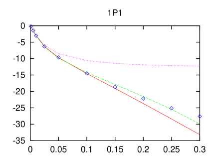
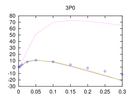
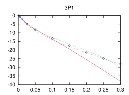
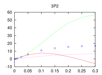
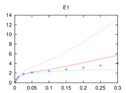
Figure 5: Predictions for the P–waves and the mixing parameter $\epsilon_{1}$ (in degrees) for nucleon laboratory energies $E_{\rm lab}$ below 300 MeV. For notations, see fig.4.

In fig.5 we show the corresponding partial waves together with the mixing parameter $\epsilon_{1}$ for the best global fit. In some cases, the differences between NLO and NNLO are modest, in ${}^{1}P_{1}$ and ${}^{3}P_{1}$ NLO is even somewhat better. That means that the chiral TPEP is too strong in these phases. Note also that in the ${}^{3}P_{1}$ phase OPEP is dominant. Thus, the inclusion of the contact interaction does not lead to a visible change. In ${}^{3}P_{2}$, NNLO is still too strong but the prediction is considerably better than the NLO one. The energy dependence of $\epsilon_{1}$ is fairly precisely described at NLO and NNLO. These results are visibly better than the ones obtained in ref.[3] or in ref.[12], the latter being a NNLO calculation in the KSW scheme. This is shown in detail in fig.6, where $\epsilon_{1}$ is plotted versus the cms nucleon momentum ($p<350$ MeV) in comparison to the Nimegen PSA and the results from refs.[12]. In the KSW approach, the pions are treated perturbatively. From these results we conclude that in the two–nucleon system, pions have to be treated non–perturbatively (if one intends to describe data above $p\simeq 150\,$MeV).

5.1.3 D– and F–waves

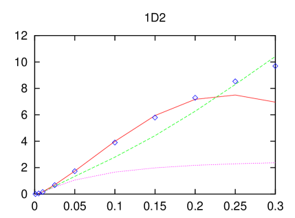
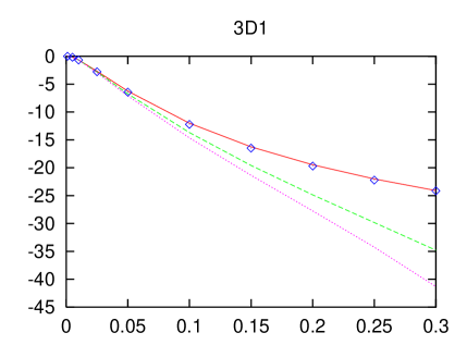
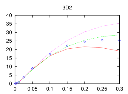
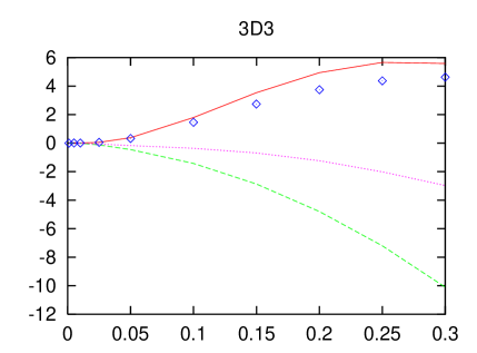
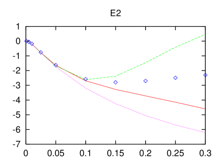
Figure 7: Predictions for the D–waves and the mixing parameter $\epsilon_{2}$ (in degrees) for nucleon laboratory energies $E_{\rm lab}$ below 300 MeV. For notations, see fig.4.

These are the most problematic phases in our approach. It is known that TPEP alone is too strong in some of these partial waves. To the order we are working, there are no contact interactions so that apart from varying the cut–off we have no freedom here. Still, for our best global fit, the D–waves are quite reasonably described, see fig.7, in particular ${}^{3}D_{1}$ and ${}^{3}D_{3}$. The result for the latter phase is rather astonishing, since e.g. in the Bonn potential [30] the correlated two–pion exchange is very important in the description of ${}^{3}D_{3}$. Such $\pi\pi$ correlations are only implicitely present to the order we are working. They are hidden in the strengths of the LECs $c_{1}$ and $c_{3}$ as explained in ref.[4]. The very accurate (and parameter-free) description of the ${}^{3}D_{1}$ wave is of course important for the deuteron channel to be discussed in section 5.2. Even in ${}^{1}D_{2}$, we get a fair description at NNLO. This partial wave is generally believed to be very sensitive to the $\Delta$–resonance. We come back to this point when we discuss the NNLO-$\Delta$ approach. Note that the D–waves are rather sensitive to the choice of the regulator cut–off, see the upper panel in fig.8. At N³LO we have besides new pion–exchange terms the first contact interactions that feed into the D–waves,

$$\langle^{m}{D}_{n}|V_{\rm cont}^{\rm{N}^{3}{\rm LO}}|^{m}{D}_{n}\rangle\sim p^{2}\,{p^{\prime}}^{2}~{}.$$ (5.4)

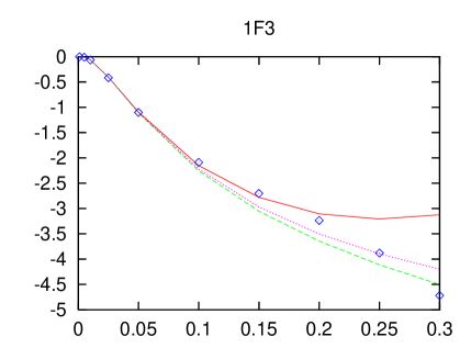
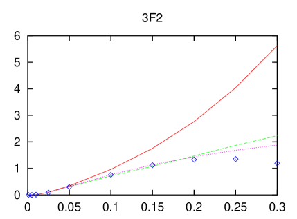
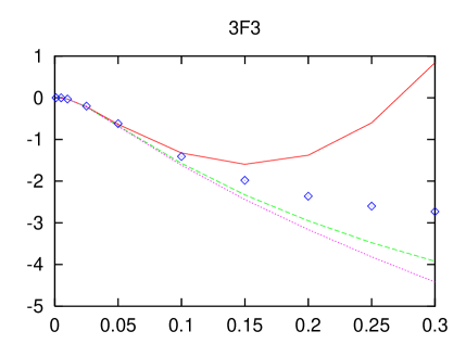
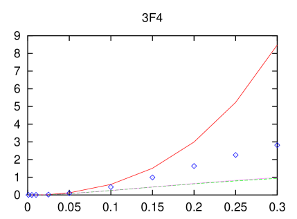
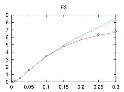
Figure 9: Predictions for the F–waves and the mixing parameter $\epsilon_{3}$ (in degrees) for nucleon laboratory energies $E_{\rm lab}$ below 300 MeV. For notations, see fig.4.

More precisely, we have one independent parameter in each D–wave. Thus the cut–off independence will be restored by the running of the corresponding LECs. To illustrate this, we show in the lower panel of fig.8 the partial N³LO results for the ${}^{1}D_{2}$ channel. The corresponding potential consists of the NNLO terms plus one N³LO contact interaction. As expected, the cut–off dependence of the phase shift is very much reduced compared to the NNLO result. Of course, this illustrative example can not substitute for a complete N³LO calculation, but one should expect very similar results. Note that according to our findings, the NNLO potential in the D–wave channels is not weak enough to be treated perturbatively, as it has been done in ref.[9]. The potential has to be iterated to all orders in the LS equation. Only then one obtains a reasonable description of the phase shifts in these partial waves. Concerning the F–waves, which are shown in fig.9, ${}^{1}F_{3}$ and $\epsilon_{3}$ are well described, whereas the NNLO TPEP is visibly too strong in ${}^{3}F_{2}$, ${}^{3}F_{3}$, and ${}^{3}F_{4}$. This can be cured at higher orders by contact interactions. More precisely, a N³LO calculation should be sufficient.

5.1.4 Peripheral waves

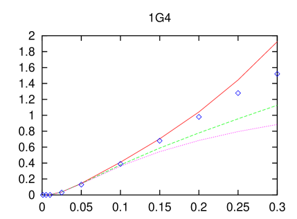
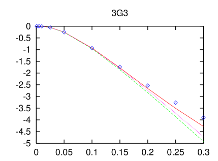
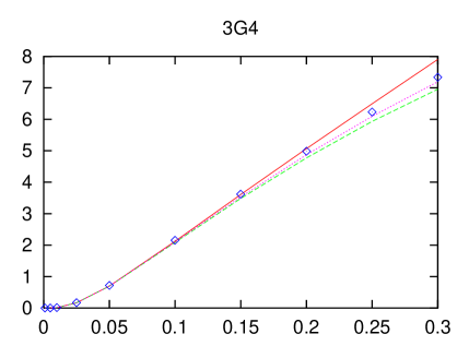
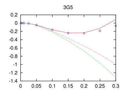
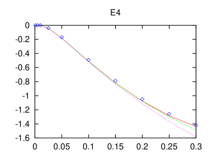
Figure 10: Predictions for the G–waves and the mixing parameter $\epsilon_{4}$ (in degrees) for nucleon laboratory energies $E_{\rm lab}$ below 300 MeV. For notations, see fig.4.

In figs.10, 11 and 12 we show the G–, H– and I–waves together with the mixing parameters $\epsilon_{4,5,6}$. These partial waves were first discussed in detail by the Munich group [9]. Their calculation was perturbative and based on dimensional regularization of the TPE graphs. However, for these partial waves the iteration becomes unimportant and our findings confirm their results. The description of ${}^{1}G_{4}$, ${}^{3}G_{3}$, ${}^{3}G_{5}$, ${}^{3}H_{5}$, ${}^{3}H_{6}$, ${}^{3}I_{5}$ and ${}^{3}I_{7}$ is visibly improved by the NNLO TPEP. Only in ${}^{1}I_{6}$ the NLO result is better than the NNLO one. Of course, for the peripheral partial waves OPE does already a fairly good job, but the improvement in some of these phases due to the NNLO TPEP clearly underlines the importance of chiral symmetry in a precise description of low–energy nuclear physics.

5.2 Deuteron properties

We now turn to the bound state properties. At NNLO (NLO), we consider an exponential regulator with $\Lambda=1.05\,(0.60)\,$GeV, which reproduces the deuteron binding energy within an accuracy of about one third of a permille (2.5 percent). We make no attempt to reproduce this number with better precision. The results for the phase shifts, which correspond to these values of the exponential regulator, are very similar to those obtained with the sharp cutoff $\Lambda=0.875\,(0.50)\,$GeV. For completeness, we list in table 5 the values of the coupling constants in the ${}^{3}S_{1}-^{3}D_{1}$ channel corresponding to the exponential regulator.

	$\tilde{C}_{{}^{3}S_{1}}$	${C}_{{}^{3}S_{1}}$	$C_{{}^{3}D_{1}-^{3}S_{1}}$
NLO	$-$0.0363	0.186	$-$0.190
NNLO	$-$14.497	15.588	$-$4.358
NNLO–$\Delta$	$-$8.637	7.264	$-$0.447

Table 5: The values of the LECs as determined from the ${}^{3}S_{1}-^{3}D_{1}$ channel. We use an exponential cut–off with $\Lambda=0.6$ GeV and 1.05 GeV at NLO and NNLO (NNLO–$\Delta$), respectively. The LEC $\tilde{C}_{{}^{3}S_{1}}$ is in $10^{4}$ GeV^-2, while the others are in $10^{4}$ GeV^-4. The parameters of the NLO, NNLO and NNLO–$\Delta$ potentials are obtained from fitting to the Nijmegen PSA.

In table 6 we collect the deuteron properties in comparison to the data and two realistic potential model predictions (the pertinent formulae are given in app. C). We give the results for NLO and NNLO. We note that deviation of our prediction for the quadrupole moment compared to the empirical value slightly larger than for the realistic potentials. The asymptotic $D/S$ ratio, called $\eta$, and the strength of the asymptotic wave function, $A_{S}$, are well described. The D–state probability, which is not an observable, is most sensitive to small variations in the cut–off. At NLO, it is comparable and at NNLO somewhat larger than obtained in the CD-Bonn or the Nijmegen-93 potential. This increased value of $P_{D}$ is related to the strong NNLO TPEP. At N³LO, we expect this to be compensated by dimension four counterterms. Altogether, we find a much improved description of the deuteron as compared to ref.[3]. Our results are almost as precise as the ones obtained in the much more complicated and less systematic meson–exchange models.

	NLO	NNLO	NNLO–$\Delta$	Nijm93	CD-Bonn	Exp.
$E_{d}$ [MeV]	$-$2.1650	$-$2.2238	$-$2.1849	$-$2.224575	$-$2.224575	$-$2.224575(9)
$Q_{d}$ [fm2]	0.266	0.262	0.268	0.271	0.270	0.2859(3)
$\eta$	0.0248	0.0245	0.0247	0.0252	0.0255	0.0256(4)
$r_{d}$ [fm]	1.975	1.967	1.970	1.968	1.966	1.9671(6)
$A_{S}$ [fm-1/2]	0.866	0.884	0.873	0.8845	0.8845	0.8846(16)
$P_{D}[\%]$	3.62	6.11	5.00	5.76	4.83	–

Table 6: Deuteron properties derived from our chiral potential compared to two “realistic” potentials (Nijmegen–93 and CD–Bonn) and the data. Here, $r_{d}$ is the root–mean–square matter radius. An exponential regulator with $\Lambda=600\,$MeV and $\Lambda=1.05\,$GeV at NLO and NNLO (NNLO–$\Delta$), in order, is used.

The coordinate space S– and D–state wave functions obtained in our approach are shown in fig.13. At NLO they look quite similar to the ones obtained from various potential models. At NNLO one obtains a lot of structure in the wave functions below 2 fm. This is because two additional spurious (unphysical) very deeply bound states appear in the ${}^{3}S_{1}-^{3}D_{1}$ channel. The binding energy of these states varies strongly by changing the cut–off. For the exponential regulator with $\Lambda=1.05\,$GeV we get binding energies of $E_{1}=47.1\,$GeV and $E_{2}=2.5\,$GeV, respectively. This values correspond to center–of–mass momenta of about a few GeV which is clearly out of the applicability range of the low–momentum effective theory. Further, because of such huge values of the binding energy these unphysical states obviously do not influence physics in the energy region below 350 MeV that we are interested in and can, in principle, be integrated out. A very similar situation with the spurious states happens at NNLO also in other S–, P– and D–waves. Note that these unphysical states are purely short range effects: as one can see from the fig.14 the wave–functions corresponding to such states become negligeble for distances above 2 fm. The corresponding root–mean–square matter radii are $\langle r_{1}^{2}\rangle^{1/2}=0.27\,$fm and $\langle r_{2}^{2}\rangle^{1/2}=0.40\,$fm. For separations above 2 fm the NNLO deuteron wave–function is very close to the one obtained with the CD-Bonn potential. This is shown in fig.15. For a discussion on such deeply bound states in effective field theories, see ref.[23]. We end this paragraph with the following remark: According to Levinson’s theorem, the difference between the phase shift at the origin and at infinity is given by $n\pi$, with $n$ the number of bound states. Thus, the phase shifts in the S–, P– and D–waves should become unphysical at large energies. This is, however, of no relevance for the EFT since we do not attempt to correctly reproduce (or predict) the phase shift behaviour for all energies (from threshold to infinity).

5.3 Results for the NNLO-$\Delta$ approach

As already stated before, our NNLO-$\Delta$ approach is not complete since we are omitting the dimension two pion–nucleon interactions not generated by the isobar. While the LECs $c_{3}$ and $c_{4}$ are dominated by the $\Delta$, see ref. [4], most of the correlated two–pion exchange is parametrized in $c_{1}$. However, we are mostly interested in investigating the role of the $\Delta$ in all partial waves and therefore keep the cut–off $\Lambda$ fixed at 875 MeV but refit the LECs $C_{i}$ (see table 1 for their values). More precisely, a best global fit leads to a very similar cut–off value as in NNLO (this is expected due to the cut–off sensitivity of the D–waves) but for better comparison we discuss here the results obtained with exactly the same value for $\Lambda$. Note also that the precision of the fits is better than NLO in the theory without $\Delta$ but somewhat worse than the corresponding NNLO fits. This is due to the absence of contributions from higher mass states encoded in the LECs $c_{1,3,4}$ not present in the NNLO–$\Delta$ approach discussed here. It goes beyond the scope of this paper to systematically include the effects of this important resonance in the framework of the EFT expansion as detailed in ref.[31]. In fact, a study of pion–nucleon scattering in that framework is not yet available and thus the corresponding LECs are not determined. Formally, we follow the Munich group [32] (for details, see app.B). Again, it is important to stress that we iterate our potential to all orders.

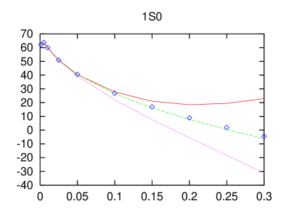
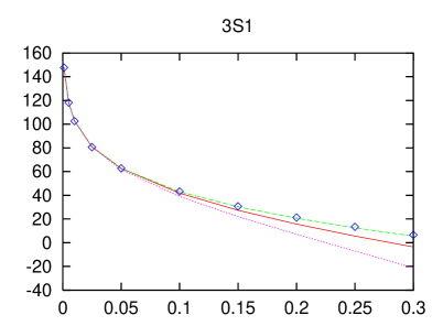
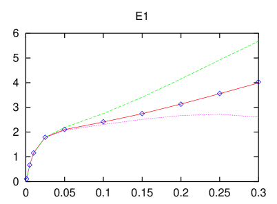
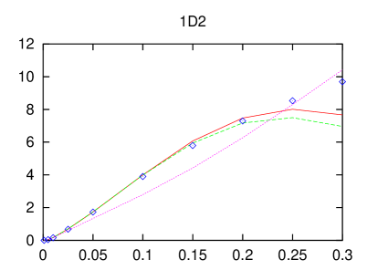
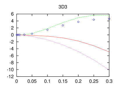
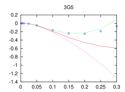
Figure 16: Phase shifts (in degrees) for the NNLO–$\Delta$ theory (red solid lines) in comparison to the NNLO (green dashed lines) and NLO (purple dotted lines) results as a function of the lab energy in GeV. For other notations, see fig.4.

Let us now discuss the results of the NNLO–$\Delta$ approach. We refrain from showing all partial waves but rather discuss some particular examples, collected in fig.16. The two S–waves shown in that figure are not very different from the NNLO result, although the description of ${}^{3}S_{1}$ is slighly worse at higher energies. All P–waves are very similar in NNLO and NNLO–$\Delta$, the most visible difference appears in $\epsilon_{1}$, as can be seen in the figure. The most dramatic effects appear in the D–waves. This is expected since these are parameter–free predictions and we had already pointed out the cut–off sensitivity in sec. 5.1.3. Interestingly, the description of ${}^{1}D_{2}$ is almost identical in the two approaches, consequently any important isobar effect in this partial wave can be well represented by contact interactions with their strength given by the coupling of the $\Delta$ to the $\pi N$ system. In ${}^{3}D_{3}$ (also shown in fig.16) the absence of the scalar–isoscalar two–pion correlations is clearly visible. Our result thus confirms a finding made already in the Bonn potential, namely that this particular partial wave is essential dominated by correlated TPE. We also note that the description of ${}^{3}D_{1}$ and ${}^{3}D_{2}$ is worse in NNLO–$\Delta$ than in NNLO. For the F–waves, the differences between the two approaches are very small, with the exception of ${}^{3}F_{4}$, which is improved in the presence of the isobar. The most significant effect in the higher partial waves shows up in ${}^{3}G_{5}$ as shown in fig.16. Clearly, two–pion correlations not related to the $\Delta$ play an important role to bring the prediction for this partial wave in agreement with the data. The deuteron properties for an exponential regulator with $\Lambda=1.05\,$GeV are listed in table 6. Most observables come out in between the NLO and NNLO results for the deltaless approach. The sole exception is the quadrupole moment, which is improved. We remark again that only after a fully systematic inclusion of the $\Delta$, one should draw quantitative conclusions. It appears, however, that simply using resonance saturation to encode the phyiscs of the isobar in the dimension two pion–nulceon LECs is a sufficient procedure in the two–nucleon sector. A truely quantitative inclusion of the delta should be done in the framework of the “small scale expansion” [31]. In that case, the leading delta effects would already appear at NLO since the nucleon–delta mass splitting is counted as a small parameter. Such an investigation is, however, beyond the scope of this article. We also note that explicit isobar degrees of freedom were considered in ref.[3]. A direct comparison with their work is, however, not possible since no separate result for fits with and without delta are given.

6 Summary

In this paper, we have calculated properties of the two–nucleon system based on a chiral effective field theory. The underlying formalism was already presented in I. The results of this investigation can be summarized as follows:

1. Based on a modified Weinberg power counting (as explained in I), we have constructed a chiral two–nucleon potential at NNLO. It consists of one– and two–pion exchange diagrams, including dimension two insertions from the effective pion–nucleon Lagrangian. The corresponding LECs have been taken from an investigation of $\pi N$ scattering [7]. In addition, there are two and seven four–nucleon contact interactions at LO and NLO, respectively. The coupling constants of these terms must be fixed by a fit to data.

2. For large momenta, the potential becomes unphysical and has to be regularized. We perform this regularization on the level of the Lippmann–Schwinger equation, as explained in sect.2 using either a sharp or an exponential regulator function. At NLO, physics does not depend on the cut–off in the range between 400 and 650 MeV. At NNLO, this range is larger and extends from 650 to 1000 MeV. This can be understood from the chiral TPEP, which at NNLO includes $\pi\pi$ correlations. These introduce a new mass scale well above twice the pion mass.

3. We have shown that the contact interactions can be combined in such a way that each combination feeds into one partial wave. More precisely, the nine four–nucleon couplings can be determined uniquely by a fit to the two S–waves, four P–waves and the mixing parameter $\epsilon_{1}$ for nucleon laboratory energies below 100 MeV. As expected from the power counting underlying the EFT, the fits improve when going from LO to NLO to NNLO, compare fig.1.

4. At NNLO, the resulting S–waves are of very high precision (for nucleon laboratory energies below 300 MeV), see e.g. tables 2,3 and fig.4. The so–called range parameters collected in table 4 agree with what is found in the phase shift analysis. The P–waves are mostly well described, in particular the mixing parameter $\epsilon_{1}$ is in good agreement with the phase shift analysis. We also note that above nucleon cms momenta of about 150 MeV, our NLO and NNLO results are far better than the one obtained in the KSW scheme at NLO and NNLO.

5. All other partial waves are free of parameters. The D–waves, in particular ${}^{3}D_{1}$ and ${}^{3}D_{3}$ are very well described. We have also discussed the cut–off sensitivity of these results. The NNLO TPEP is too strong in the triplet F–waves. This is expected to be cured at N³LO due to the appearance of dimension four contact terms. For the peripheral waves, we recover the results of the Munich group [9], namely that in most cases OPE works well but chiral NNLO TPEP clearly improves the description of some partial waves like e.g. ${}^{3}G_{5}$, ${}^{3}H_{5}$ or ${}^{3}I_{7}$.

6. The deuteron properties are mostly well described, at NLO and NNLO, compare table 6. At NNLO, the deuteron wave functions shows some interesting structure due to the appearance of two very deeply bound states. These are an artefact of the NNLO approximation. They have no influence on low energy properties and can be completely projected out from the theory. Our precise deuteron wavefunctions can be used for pion photoproduction, pion–deuteron scattering or Compton scattering off deuterium (still, the hybrid approach proposed by Weinberg [33] remains a useful tool).

7. We have also considered an approach with explicit $\Delta$ degrees of freedom in the TPEP. This NNLO–$\Delta$ approach is very similar to the NNLO results in the theory without isobars, with the exception of the partial waves that are sensitive to pionic scalar–isoscalar correlations like e.g. ${}^{3}D_{3}$. We conclude that the inclusion of the $\Delta$ via resonance saturation of the dimension two $\pi N$ LECs captures the essential physics of the isobar in the two–nucleon system. We note, however, that a more systematic study of pion–nucleon scattering in an EFT including the $\Delta$ is needed to further quantify these statements.

Our findings do not only show that the scheme originally proposed by Weinberg works quantitatively, it even works much better than it was expected. It extends the succesfull applications of effective field theory (chiral perturbation theory) in the pion and pion–nucleon sectors to systems with more than one nucleon. Clearly, one should now reconsider processes, which have been evaluated using Weinberg’s hybrid approach [33] ($\pi-d$ scattering [33, 34], $\gamma d\to\pi^{0}d$ [35], $\gamma d\to\gamma d$ [36]) and extend these considerations to systems with more than two nucleons. First steps in that direction within the potential approach can be found in recent works [37, 38]. In addition, a fresh look at charge symmetry and charge independence breaking is called for (for earlier studies, see e.g. refs.[39, 40, 41]). Work along these lines is underway. Furthermore, the precise relation to the KSW scheme, which has been shown to be successfull at low energies, has to be worked out.

Appendix A The renormalization procedure

In this appendix we spell out some details about the renormalization procedure mentioned briefly in sect.2. We will use the divergent loop integrals $J_{0,2,4}$ defined in eq.(2.1) to express all divergences and remove these by proper subtractions and redefinitions of physical quantities.

We consider first the one–loop corrections to the OPEP. These were given in eq.(4.33) of I. We rewrite this expression here using different conventions for the isospin operators and the pion decay constant

$$V^{(2)}_{1\pi,\,{\rm 1-loop}} = \frac{g_{A}^{4}}{(2f_{\pi})^{4}}\,(\vec{\tau}_{1}\cdot\vec{\tau}_{2})\,\frac{1}{\omega_{q}^{2}}\,\int\,\frac{d^{3}l}{(2\pi)^{3}}\,\frac{1}{\omega_{l}^{3}}\,\Bigg{\{}(\vec{l}\cdot\vec{q}\,)\Big{(}(\vec{\sigma}_{1}\cdot\vec{l}\,)\,(\vec{\sigma}_{2}\cdot\vec{q}\,)+(\vec{\sigma}_{1}\cdot\vec{q}\,)\,(\vec{\sigma}_{2}\cdot\vec{l}\,)\Big{)}$$

$$\qquad\qquad\qquad\qquad\qquad\qquad\qquad\qquad+2{\vec{l}\,}^{2}\,(\vec{\sigma}_{1}\cdot\vec{q}\,)\,(\vec{\sigma}_{2}\cdot\vec{q}\,)\Bigg{\}}\,\,\,,$$

$$= \frac{g_{A}^{4}}{(2f_{\pi})^{4}}\,(\vec{\tau}_{1}\cdot\vec{\tau}_{2})\,\frac{8}{3}\,(\vec{\sigma}_{1}\cdot\vec{q}\,)\,(\vec{\sigma}_{2}\cdot\vec{q}\,)\,\frac{1}{\omega_{q}^{2}}\,\int\,\frac{d^{3}l}{(2\pi)^{3}}\,\frac{l^{2}}{\omega_{l}^{3}}$$

$$= \frac{g_{A}^{4}}{48\pi^{2}f_{\pi}^{4}}\,(\vec{\tau}_{1}\cdot\vec{\tau}_{2})\,(\vec{\sigma}_{1}\cdot\vec{q}\,)\,(\vec{\sigma}_{2}\cdot\vec{q}\,)\,\frac{1}{\omega_{q}^{2}}\,\biggl{\{}5M_{\pi}^{2}+3M_{\pi}^{2}\ln\frac{M_{\pi}^{2}}{4\epsilon^{2}}+4J_{2}-6M_{\pi}^{2}J_{0}\biggr{\}}~{},$$

in terms of the two divergent loop functions $J_{0,2}$ defined in eq.(2.1). Therefore, this contribution has exactly the same form as the OPEP (renormalized OPE),

$$V_{1\pi}^{(0)}+V_{1\pi}^{(2)}=V_{1\pi}^{\rm r}~{},$$ (A.2)

provided we redefine the coupling constant $g_{A}^{0}$ (the superscript “0” denotes the leading term in the chiral expansion) in the following way:

$$(g_{A}^{r})^{2}=(g_{A}^{0})^{2}-\frac{(g_{A}^{0})^{4}}{12\pi^{2}f_{\pi}^{2}}\biggl{\{}5M_{\pi}^{2}+3M_{\pi}^{2}\ln\frac{M_{\pi}^{2}}{4\epsilon^{2}}+4J_{2}-6M_{\pi}^{2}J_{0}\biggr{\}}~{}.$$ (A.3)

Clearly, $g_{A}^{r}$ and $g_{A}^{0}$ differ by terms of second order in the chiral dimension. Consequently, all NLO one–loop corrections to OPEP can be taken care off by renormalization of $g_{A}^{0}$.

In addition, there are the one–loop corrections to the lowest order four–fermion interactions, cf. eq.(4.34) of I. Performing spin averaging, the corresponding contribution can be expressed in terms of the divergent loop functions $J_{0,2}$ as

$$V_{{\rm NN,1-loop}}^{(2)} = -\frac{g_{A}^{2}}{6\pi^{2}f_{\pi}^{2}}\,C_{T}^{0}\,(3-\vec{\tau}_{1}\cdot\vec{\tau}_{2})\,(\vec{\sigma}_{1}\cdot\vec{\sigma}_{2})\,\int\,d^{3}l\,l^{4}\,\omega_{l}^{-3}$$

$$= -\frac{g_{A}^{2}}{24\pi^{2}f_{\pi}^{2}}\,C_{T}^{0}\,(3-\vec{\tau}_{1}\cdot\vec{\tau}_{2})\,(\vec{\sigma}_{1}\cdot\vec{\sigma}_{2})\,\biggl{\{}5M_{\pi}^{2}+3M_{\pi}^{2}\ln\frac{M_{\pi}^{2}}{4\epsilon^{2}}+4J_{2}-6M_{\pi}^{2}J_{0}\biggr{\}}~{}.$$

or in a more compact notation

$$V_{{\rm NN,1-loop}}^{(2)}=-3S\,(\vec{\sigma}_{1}\cdot\vec{\sigma}_{2})+S\,(\vec{\sigma}_{1}\cdot\vec{\sigma}_{2})(\vec{\tau}_{1}\cdot\vec{\tau}_{2})~{},$$ (A.5)

with

$$S=\frac{g_{A}^{2}}{24\pi^{2}f_{\pi}^{2}}\,C_{T}^{0}\,\biggl{\{}5M_{\pi}^{2}+3M_{\pi}^{2}\ln\frac{M_{\pi}^{2}}{4\epsilon^{2}}+4J_{2}-6M_{\pi}^{2}J_{0}\biggr{\}}~{}.$$ (A.6)

Antisymmetrization allows to map the two spin–isospin operators appearing in eq.(A.5) onto the two non–derivative operators used in $V^{(0)}_{NN}$, cf. eq.(2). Therefore, the effect of the one–loop corrections to the lowest order four–nucleon contact interactions can be completely absorbed by renormalizing the constants $C_{S}^{0}$ and $C_{T}^{0}$,

$$C_{S}^{r}=C_{S}^{0}-3S~{},\quad C_{T}^{r}=C_{T}^{0}-3S~{}.$$ (A.7)

We note that further renormalization of these couplings is due to the two–pion exchange, as dicussed below.

A similar procedure also works for the one–loop TPE graphs, cf. eq.(4.30) of I. In fact, the NLO TPEP renormalizes the various dimension zero and two coupling constants $C_{i}$. So as not to repeat the argument, we simply give the relevant momentum space integrals in terms of $J_{0,2}$ and $J_{4}$,

$$\int\,\frac{d^{3}l}{(2\pi)^{3}}\,\frac{1}{\omega_{+}\omega_{-}(\omega_{+}+\omega_{-})} = -\frac{1}{8\pi^{2}}\,\biggl{\{}\frac{s}{q}\ln\frac{s+q}{s-q}+\ln\frac{M_{\pi}^{2}}{\epsilon^{2}}-2J_{0}\biggr{\}}~{},$$ (A.8)

$$\int\,\frac{d^{3}l}{(2\pi)^{3}}\,\frac{l^{2}}{\omega_{+}\omega_{-}(\omega_{+}+\omega_{-})} = \frac{1}{24\pi^{2}}\,\biggl{\{}\frac{2s^{3}}{q}\ln\frac{s+q}{s-q}+(14M_{\pi}^{2}-q^{2})+2(9M_{\pi}^{2}+q^{2})\ln\frac{M_{\pi}^{2}}{\epsilon^{2}}$$ (A.9)

$$\quad\qquad\qquad+6J_{2}-4(9M_{\pi}^{2}+q^{2})J_{0}\biggr{\}}~{},$$

$$\int\,\frac{d^{3}l}{(2\pi)^{3}}\,\frac{l^{4}+q^{4}}{\omega_{+}\omega_{-}(\omega_{+}+\omega_{-})} = \frac{1}{24\pi^{2}}\,\biggl{\{}\frac{1}{5qs}(512M_{\pi}^{6}+384M_{\pi}^{4}q^{2}+156M_{\pi}^{2}q^{4}+23q^{6})\ln\frac{s+q}{s-q}$$

$$+ \frac{1}{10}(-898M_{\pi}^{4}+192M_{\pi}^{2}q^{2}+q^{4})-\frac{1}{5}(450M_{\pi}^{4}+50M_{\pi}^{2}q^{2}+23q^{4})\ln\frac{M_{\pi}^{2}}{\epsilon^{2}}$$

$$+ 6J_{4}-4(9M_{\pi}^{2}+q^{2})J_{2}+\frac{2}{5}(450M_{\pi}^{4}+50M_{\pi}^{2}q^{2}+23q^{4})J_{0}\biggr{\}}~{},$$

$$\int\,\frac{d^{3}l}{(2\pi)^{3}}\,\frac{(q\cdot l)^{2}}{\omega_{+}\omega_{-}(\omega_{+}+\omega_{-})} = \frac{1}{8\pi^{2}}\,\biggl{\{}2M_{\pi}^{2}q^{2}\ln\frac{M_{\pi}^{2}}{\epsilon^{2}}-\frac{q^{4}}{5}+\frac{10}{3}q^{2}M_{\pi}^{2}+\frac{2}{3}q^{2}J_{2}-4M_{\pi}^{2}q^{2}J_{0}\biggr{\}}~{},$$

$$\int\,\frac{d^{3}l}{(2\pi)^{3}}\,\frac{(\omega_{+}-\omega_{-})^{2}}{\omega_{+}\omega_{-}(\omega_{+}+\omega_{-})} = \frac{1}{6\pi^{2}}\,\biggl{\{}-\frac{s^{3}}{q}\ln\frac{s+q}{s-q}-q^{2}\ln\frac{M_{\pi}^{2}}{\epsilon^{2}}+8M_{\pi}^{2}+2q^{2}J_{0}\biggr{\}}~{},$$ (A.12)

with $s=\sqrt{4M_{\pi}^{2}+q^{2}}$ and $\omega_{\pm}$ given in eq.(4.24) of I. All other integrals appearing in the 1–loop NLO TPEP can be deduced from these expressions by taking proper linear combinations or differentiation with respect to $M_{\pi}^{2}$. Putting pieces together, the expression for $V^{(2)}_{2\pi,{\rm 1-loop}}$ takes the form

$$V^{(2)}_{2\pi,{\rm 1-loop}}=V^{\rm TPEP}_{\rm NLO}+(S_{1}+S_{2}\,q^{2})\,(\vec{\tau}_{1}\cdot\vec{\tau}_{2})+S_{3}\,\biggl{[}(\vec{\sigma}_{1}\cdot\vec{q}\,)\,(\vec{\sigma}_{2}\cdot\vec{q}\,)-(\vec{\sigma}_{1}\cdot\vec{\sigma}_{2})\,q^{2}\biggr{]}~{},$$ (A.13)

with

$$S_{1} = \frac{1}{384\pi^{2}f_{\pi}^{4}}\biggl{\{}-18M_{\pi}^{2}(5g_{A}^{4}-2g_{A}^{2})\ln\frac{M_{\pi}}{\varepsilon}-M_{\pi}^{2}(61g_{A}^{4}-14g_{A}^{2}+4)$$ (A.14)

$$\qquad\qquad\qquad\qquad\qquad\qquad+18M_{\pi}^{2}(5g_{A}^{4}-2g_{A}^{2})J_{0}-3(3g_{A}^{4}-2g_{A}^{2})J_{2}\biggr{\}}~{},$$

$$S_{2} = \frac{1}{384\pi^{2}f_{\pi}^{4}}\biggl{\{}(-23g_{A}^{4}+10g_{A}^{2}+1)\ln\frac{M_{\pi}}{\varepsilon}-(13g_{A}^{4}+2g_{A}^{2})+(23g_{A}^{4}-10g_{A}^{2}-1)J_{0}\biggr{\}},$$ (A.15)

$$S_{3} = -\frac{3g_{A}^{4}}{64\pi^{2}f_{\pi}^{4}}\biggl{\{}\ln\frac{M_{\pi}}{\varepsilon}+\frac{1}{3}+J_{0}\biggr{\}}~{},$$ (A.16)

and the non–polynomial part $V^{\rm TPEP}_{\rm NLO}$ is given in eq.(2.12). The polynomial terms clearly renormalize the coupling constants of the dimension zero and two four–nucleon contact terms. Again, we perform antisymmetrization to map the terms appearing in eq.(A.13) onto the basis used in $V_{NN}^{(0,2)}$, cf. eq.(2). Including the contribution from eq.(A.7), the complete renormalization of the four–nucleon couplings takes the form

$$C_{T}^{r} = C_{T}^{0}-3S-S_{1}~{},\quad C_{S}^{r}=C_{S}^{0}-3S-2S_{1}~{},$$

$$C_{1}^{r} = C_{1}^{0}-S_{2}~{},\quad C_{2}^{r}=C_{2}^{0}-4S_{2}~{},\quad C_{3}^{r}=C_{3}^{0}-S_{3}~{},$$

$$C_{4}^{r} = C_{4}^{0}-4S_{2}~{},\quad C_{5}^{r}=C_{5}^{0}~{},\quad C_{6}^{r}=C_{6}^{0}+S_{3}~{},\quad C_{7}^{r}=C_{7}^{0}~{}.$$ (A.17)

Note that $C_{5}$ and $C_{7}$ do not get renormalized to this order. All coupling constants appearing in the main text are understood as the renormalized quantities discussed here.

Appendix B Inclusion of the $\Delta(1232)$

The inclusion of the $\Delta(1232)$ in the TPEP has been worked out in ref.[32]. For completeness, we collect here the pertinent formulae. There are three distint contributions.

$\Delta$–excitation in the triangle graphs:

$$V^{\rm TPEP}_{\Delta,\,{\rm triangle}}=-\frac{g_{A}^{2}}{192\pi^{2}f_{\pi}^{4}}\,(\vec{\tau}_{1}\cdot\vec{\tau}_{2})\,\biggl{\{}(6E-s^{2})L(q)+12\Delta^{2}ED(q)\biggr{\}}~{},$$ (B.1)

with

$$L(q) = \frac{s}{q}\ln\frac{s+q}{2M_{\pi}}~{},$$ (B.2)

$$D(q) = \frac{1}{\Delta}\,\int_{2M_{\pi}}^{\infty}\frac{d\mu}{\mu^{2}+q^{2}}\,\arctan\frac{\sqrt{\mu^{2}-4M_{\pi}^{2}}}{2\Delta}~{},$$ (B.3)

$$\Delta = m_{\Delta}-m=293~{}{\rm MeV}~{},$$ (B.4)

$$E = 2M_{\pi}^{2}+q^{2}-2\Delta^{2}~{}.$$ (B.5)

Single $\Delta$–excitation in the box graphs:

$$V^{\rm TPEP}_{\Delta,\,{\rm box}-1} = -\frac{3g_{A}^{4}}{32\pi f_{\pi}^{4}\Delta}\,(2M_{\pi}^{2}+q^{2})^{2}\,A(q)$$ (B.6)

$$- \frac{g_{A}^{4}}{192\pi^{2}f_{\pi}^{4}}\,(\vec{\tau}_{1}\cdot\vec{\tau}_{2})\,\biggl{\{}(12\Delta^{2}-20M_{\pi}^{2}-11q^{2})L(q)+6E^{2}D(q)\biggr{\}}$$

$$- \frac{3g_{A}^{4}}{128\pi^{2}f_{\pi}^{4}}\,\biggl{(}(\vec{\sigma}_{1}\cdot\vec{q}\,)(\vec{\sigma}_{2}\cdot\vec{q}\,)-q^{2}(\vec{\sigma}_{1}\cdot\vec{\sigma}_{2})\biggr{)}\,\biggl{\{}-2L(q)+(s^{2}-4\Delta^{2})D(q)\biggr{\}}$$

$$- \frac{g_{A}^{4}}{128\pi f_{\pi}^{4}\Delta}\,(\vec{\tau}_{1}\cdot\vec{\tau}_{2})\,\biggl{(}(\vec{\sigma}_{1}\cdot\vec{q}\,)(\vec{\sigma}_{2}\cdot\vec{q}\,)-q^{2}(\vec{\sigma}_{1}\cdot\vec{\sigma}_{2})\biggr{)}\,s^{2}\,A(q)~{},$$

with $A(q)$ given in eq.(2.13).

Double $\Delta$–excitation in the box graphs:

$$V^{\rm TPEP}_{\Delta,\,{\rm box}-2} = -\frac{3g_{A}^{4}}{64\pi^{2}f_{\pi}^{4}}\,\biggl{\{}-4\Delta^{2}L(q)+E[H(q)+(E+8\Delta^{2})D(q)]\biggr{\}}$$

$$- \frac{g_{A}^{4}}{384\pi^{2}f_{\pi}^{4}}\,(\vec{\tau}_{1}\cdot\vec{\tau}_{2})\,\biggl{\{}(12E-s^{2})L(q)+3E[H(q)+(8\Delta^{2}-E)D(q)]\biggr{\}}$$

$$- \frac{3g_{A}^{4}}{512\pi^{2}f_{\pi}^{4}}\,\biggl{(}(\vec{\sigma}_{1}\cdot\vec{q}\,)(\vec{\sigma}_{2}\cdot\vec{q}\,)-q^{2}(\vec{\sigma}_{1}\cdot\vec{\sigma}_{2})\biggr{)}\,\biggl{\{}6L(q)+(12\Delta^{2}-s^{2})D(q)\biggr{\}}$$

$$- \frac{g_{A}^{4}}{1024\pi^{2}f_{\pi}^{4}}\,(\vec{\tau}_{1}\cdot\vec{\tau}_{2})\,\biggl{(}(\vec{\sigma}_{1}\cdot\vec{q}\,)(\vec{\sigma}_{2}\cdot\vec{q}\,)-q^{2}(\vec{\sigma}_{1}\cdot\vec{\sigma}_{2})\biggr{)}\,\biggl{\{}2L(q)+(4\Delta^{2}+s^{2})D(q)\biggr{\}}~{},$$

with

$$H(q)=\frac{2E}{s^{2}-4\Delta^{2}}\biggl{[}L(q)-L(2\sqrt{\Delta^{2}-M_{\pi}^{2}})\biggr{]}\quad.$$ (B.8)

Finally, let us show how to arrive at the coupling constant relation given in eq.(2.16). In spin–isopsin SU(4) (or more generally, SU(6)), one obtains

$$g_{\Delta N\pi}=\frac{3}{\sqrt{2}}\,g_{\pi N}~{}.$$ (B.9)

Using now the Goldberger–Treiman relation

$$g_{\pi N}=g_{A}\,\frac{m}{F_{\pi}}~{},$$ (B.10)

one arrives at eq.(2.16). The numerical value of $g_{\Delta N\pi}$ follows from using $g_{A}=1.26$. Note that this value for the coupling constant leads to a $\Delta$–width of about 117 MeV.

Appendix C Formulae for the deuteron properties

Here, we collect the formulae needed to calculate the deuteron properties. Denote by $u(r)$ and $w(r)$ the S– and D–wave coordinate space wave functions. We denote the momentum space representations of $u(r)/r$ and $w(r)/r$ by $\tilde{u}(p)$ and $\tilde{w}(p)$, respectively. We have

$${\rm Normalization} : \int_{0}^{\infty}dp\,p^{2}\,[\tilde{u}(p)^{2}+\tilde{w}(p)^{2}]=\int_{0}^{\infty}dr\,[{u}(r)^{2}+{w}(r)^{2}]=1~{},$$ (C.1)

$${\rm D-state~{}probability} : \int_{0}^{\infty}dp\,p^{2}\,\tilde{w}(p)^{2}=\int_{0}^{\infty}dr\,w(r)^{2}~{},$$ (C.2)

$${\rm Quadrupole~{}moment} : Q_{d}=\frac{1}{20}\int_{0}^{\infty}dr\,r^{2}\,w(r)\,[\sqrt{8}u(r)-w(r)]$$ (C.3)

$$\quad\,\,\,=-\frac{1}{20}\int_{0}^{\infty}dp\biggl{\{}\sqrt{8}\biggl{[}p^{2}\frac{d\tilde{u}(p)}{dp}\frac{d\tilde{w}(p)}{dp}+3p\tilde{w}(p)\frac{d\tilde{u}(p)}{dp}\biggr{]}$$

$$\qquad\qquad\qquad\qquad\qquad\qquad+p^{2}\biggl{(}\frac{d\tilde{w}(p)}{dp}\biggr{)}^{2}+6\tilde{w}(p)^{2}\biggr{\}}~{},$$

$${\rm Asymptotic~{}S-state} : u(r)\to A_{S}\,{\rm e}^{-\gamma\,r}\quad{\rm for}~{}r\to\infty~{},$$ (C.4)

$${\rm Asymptotic~{}D/S-ratio}~{}\eta : w(r)\to\eta\,A_{S}\,\biggl{(}1+\frac{3}{\gamma r}+\frac{3}{(\gamma r)^{2}}\biggr{)}\,{\rm e}^{-\gamma\,r}\quad{\rm for}~{}r\to\infty~{},$$ (C.5)

$${\rm RMS~{}(matter)~{}radius} : r_{d}=\frac{1}{2}\,\biggl{[}\,\int_{0}^{\infty}dr\,r^{2}\,[{u}(r)^{2}+{w}(r)^{2}]\,\biggr{]}^{1/2}~{},$$ (C.6)

with $\gamma=\sqrt{m\,|E_{d}|}=45.7\,$MeV (using $m=(m_{p}+m_{n})/2)$. Note that the momentum–space representation of $Q_{d}$ given in eq.(C.3) shows why one cannot use a sharp momentum–space regulator to calculate this quantity. We also remark that the D–state probability is not an observable. Meson–exchange current corrections to $Q_{d}$ are not given.

Figures

Figure 2: Running of the four–nucleon coupling constants in the ${}^{1}S_{0}$ (upper panel) and ${}^{3}S_{1}-^{3}D_{1}$ (lower panel) partial waves. In the upper panel, the solid red (dashed blue) line refers to $C_{{}^{1}S_{0}}$ ($\tilde{C}_{{}^{1}S_{0}}$). In the lower panel, the solid red (dashed blue) line refers to $C_{{}^{3}S_{1}}$ ($\tilde{C}_{{}^{3}S_{1}}$). The green (dashed–dotted) line refers to the constant in the coupled ${}^{3}S_{1}-^{3}D_{1}$ system. The units are the same as in the table 1.

Figure 3: Phase shifts for the two solutions in the ${}^{1}S_{0}$–wave as dicussed in the text. At NLO (upper panel), these are indistinguishable. At NNLO (lower panel), one of the solutions (black line) shows an unacceptable behaviour at higher momenta and is discarded.

Figure 4: Predictions for the S–waves (in degrees) for nucleon laboratory energies $E_{\rm lab}$ below 300 MeV (0.3 GeV). The purple dotted, green dashed and red solid curves represent LO, NLO and NNLO results, in order. The blue squares depict the Nijmegen PSA results. In the upper and the lower panel, ${}^{1}S_{0}$ and ${}^{3}S_{1}$, respectively, are shown.

Figure 6: Predictions for the mixing parameter $\epsilon_{1}$ for nucleon cms momenta $p$ below 350 MeV. The green, blue and red solid curves represent our LO, NLO and NNLO results, in order. For comparison, the NLO [11] and NNLO [12] results in the KSW scheme are also shown. The black squares depict the Nijmegen PSA results.

Figure 8: The ${}^{1}D_{2}$ partial wave at NNLO for three different values of the cut–off $\Lambda$ (upper panel) and at N³LO (lower panel). The blue diamonds are the result of the Nijmegen partial wave analysis.

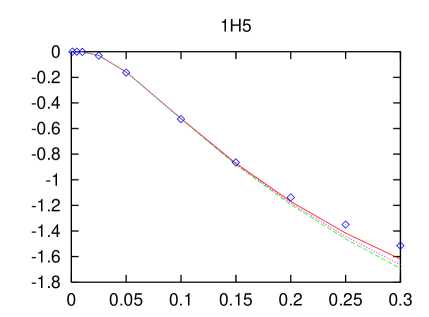
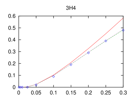
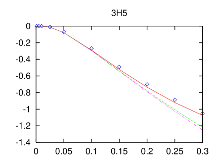
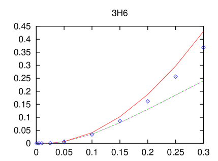
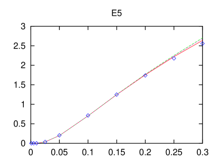
Figure 11: Predictions for the H–waves and the mixing parameter $\epsilon_{5}$ (in degrees) for nucleon laboratory energies $E_{\rm lab}$ below 300 MeV. For notations, see fig.4.

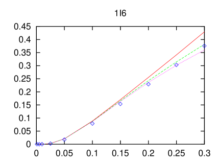
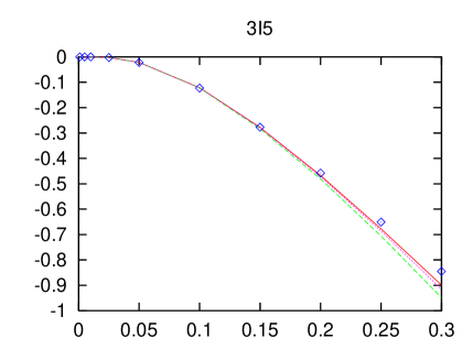
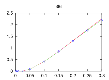
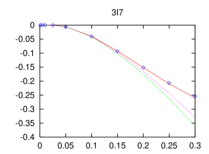
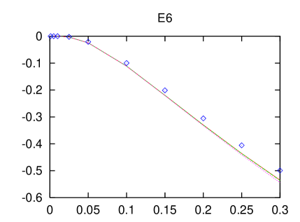
Figure 12: Predictions for the I–waves and the mixing parameter $\epsilon_{6}$ (in degrees) for nucleon laboratory energies $E_{\rm lab}$ below 300 MeV. For notations, see fig.4.

Figure 13: Coordinate space representations of the S– (red solid line) and D–wave (blue dashed line) deuteron wave functions at NLO (upper panel) and NNLO (lower panel).

Figure 14: Coordinate space representations of the S– (red solid line) and D–wave (blue dashed line) for the two unphysical boundstates.

Figure 15: Coordinate space representations of the S– (upper panel) and D–wave (lower panel) deuteron wave functions at NNLO compared to the one from the CD-Bonn potential.

References

- [1] E. Epelbaoum, W. Glöckle and Ulf-G. Meißner, Nucl. Phys. A637 (1998) 107.
- [2] S. Weinberg, Nucl. Phys. B363 (1991) 3.
- [3] C. Ordóñez, L. Ray and U. van Kolck, Phys. Rev. C53 (1996) 2086.
- [4] V. Bernard, N. Kaiser and Ulf-G. Meißner, Nucl. Phys. A615 (1997) 483.
- [5] M. Mojžiš, Eur. Phys. J. C2 (1998) 181.
- [6] N. Fettes, Ulf-G. Meißner and S. Steininger, Nucl. Phys. A640 (1998) 199.
- [7] P. Büttiker and Ulf-G. Meißner, hep-ph/9908247.
- [8] T.-S. Park et al. Nucl. Phys. A646 (1999) 83.
- [9] N. Kaiser, R. Brockmann and W. Weise, Nucl. Phys. A625 (1997) 758.
- [10] M.R. Robilotta and C.A. da Rocha, Nucl. Phys. A615 (1997) 391.
- [11] D.B. Kaplan, M.J. Savage and M.B. Wise, Nucl. Phys. B534 (1998) 329.
- [12] S. Fleming, T. Mehen and I.W. Stewart, nucl-th/9906056.
- [13] G. Rupak and N. Shoresh, nucl-th/9902077; nucl-th/9906077.
- [14] M.C.M. Rentmeester et al., Phys. Rev. Lett. 82 (1999) 4992.
- [15] W. Glöckle, The Quantum Mechanical Few-Body Problem, Springer Verlag, Heidelberg, 1983.
- [16] K. Erkelenz, R. Alzetta and K. Holinde, Nucl. Phys. A176 (1971) 413.
- [17] H.P. Stapp, T.J. Ypsilantis and N. Metropolis, Phys. Rev. 105 (1957) 302.
- [18] M.C.M. Rentmeester, private communication.
- [19] J.J. de Swart, C.P.F. Terheggen, V.G.J. Stoks, nucl-th/9509032.
- [20] V.G.J. Stoks et al., Phys. Rev. C48 (1993) 792.
- [21] SAID online–program (Virginia Tech Partial-Wave Analysis Facility), R.A. Arndt et al., htpp://said.phys.vt.edu.
- [22] V.G.J. Stoks et al., Phys. Rev. C49 (1994) 2950.
- [23] G.P. Lepage, nucl-th/9706029.
- [24] C.H. Hyun, D.–P. Min and T.–S. Park, nucl-th/9908073.
- [25] S.R. Beane, T.D. Cohen and D.R. Philipps, Nucl. Phys. A632 (1998) 445.
- [26] R.B. Wiringa et al., Phys. Rev. C51 (1995) 38.
- [27] R. Machleidt, F. Sammarruca and Y. Song, Phys. Rev. C53 (1996) R1483.
- [28] T.D. Cohen and J.M. Hansen, Phys. Rev. C59 (1999) 13.
- [29] G. Ecker and Ulf-G. Meißner, Comments Nucl. Part. Phys. 21 (1995) 347.
- [30] R. Machleidt, K. Holinde and Ch. Elster, Phys. Rep. 149 (1987) 1.
- [31] T.R. Hemmert, B.R. Holstein and J. Kamber, J. Phys. G34 (1998) 1831.
- [32] N. Kaiser, S. Gerstendörfer and W. Weise, Nucl. Phys. A637 (1998) 635.
- [33] S. Weinberg, Phys. Lett. B295 (1992) 114.
- [34] S.R. Beane, V. Bernard, T.-S.H. Lee and Ulf-G. Meißner, Phys. Rev. C57 (1998) 424.
- [35] S.R. Beane, V. Bernard, T.-S.H. Lee, Ulf-G. Meißner and U. van Kolck, Nucl. Phys. A618 (1997) 381.
- [36] S.R. Beane, M. Malheiro, D.R. Phillips and U. van Kolck, nucl-th/9905023.
- [37] J.L. Friar, D. Hüber, H. Witala and G.L. Payne, nucl-th/9908058.
- [38] D. Hüber, J.L. Friar, A. Nogga, H. Witala and U. van Kolck, nucl-th/9910034.
- [39] U. van Kolck, Phys. Rev. C49 (1994) 2932.
- [40] U. van Kolck et al., Phys. Rev. Lett. 80 (1998) 4386.
- [41] E. Epelbaum and Ulf-G. Meißner, Phys. Lett. B461 (1999) 287.