Numerical renormalization using dimensional regularization: a simple test case in the Lippmann-Schwinger equation

Abstract

Dimensional regularization is applied to the Lippmann-Schwinger equation for a separable potential which gives rise to logarithmic singularities in the Born series. For this potential a subtraction at a fixed energy can be used to renormalize the amplitude and produce a finite solution to the integral equation for all energies. This can be done either algebraically or numerically. In the latter case dimensional regularization can be implemented by solving the integral equation in a lower number of dimensions, fixing the potential strength, and computing the phase shifts, while taking the limit as the number of dimensions approaches three. We demonstrate that these steps can be carried out in a numerically stable way, and show that the results thereby obtained agree with those found when the renormalization is performed algebraically to four significant figures.

I Introduction

One difficulty for standard treatments of hadronic reactions is that form factors are introduced at hadronic vertices in order to regulate integrals which would otherwise be divergent. This procedure reflects the substructure of hadrons which gives them a finite extent, and hence a form factor. However, any field theory upon which such calculations are based will necessarily be non-local. The implementation of basic field theoretic principles, such as causality and electromagnetic gauge invariance, is quite involved in such field theories [1, 2]. Methods which impose gauge invariance on an amplitude containing hadronic form factors have been formulated,[3, 4, 5] but they are intrinsically non-unique, since they constrain only the longitudinal part of the photon’s coupling to the hadronic system.

Some of these difficulties can be resolved by using dimensional regularization (DR)[6, 7, 8, 9] to render divergent integrals finite. This is the method of choice for dealing with the infinities which arise in perturbative field theoretic calculations. However, there are very few studies of the application of dimensional regularization to integral equations. One notable exception is the recent application of DR to a Schwinger-Dyson equation in quenched QED by Schreiber et al.[10]. In this paper we adapt their method and apply it to the Lippmann-Schwinger (LS) equation.

We consider one member of the class of potentials in which one subtraction at a fixed energy results in a finite integral equation at all energies. The potential we choose is separable and so provides a toy problem where the renormalized amplitude can be derived algebraically in a straightforward way. The amplitude thereby obtained can then be compared with that found by the numerical solution of the dimensionally-regulated integral equation. We will show that with careful numerical work the phase shifts obtained via these two different methods are in excellent agreement with each other. This proves that many of the difficulties associated with implementing dimensional regularization numerically can be overcome, and hence that such “numerical dimensional regularization and renormalization” facilitates the extraction of finite phase shifts from a particular class of divergent potentials.

In Sec. II we outline the general framework for implementing dimensional regularization and renormalization techniques numerically in the LS equation. We show how the LS equation can be analytically continued to lower numbers of dimensions, $D=3-\epsilon$, thus ameliorating the divergences which appear in three dimensions. The application of a renormalization condition at one energy in $3-\epsilon$ dimensions can then lead to an amplitude which is finite at all energies in this lower number of dimensions, and thence to an amplitude which is well-defined as the limit $\epsilon\rightarrow 0$ is taken. In Sec. III the special case of a separable potential, which leads to a divergent amplitude as $\epsilon\rightarrow 0$ is considered. We obtain the amplitude for this potential for $\epsilon>0$. Renormalizing the amplitude by demanding that the binding energy of the deuteron be reproduced leads to a divergence in the inverse of the “bare” coupling which appears in the original separable potential. We show that in DR this divergence goes as $1/\epsilon$. We then observe that for this particular potential, it is not necessary to use DR, since the problem can be subtractively renormalized. That is to say, a subtraction at one energy, which can be carried out algebraically, renders the amplitude finite at all energies.

However, it is not generally true that such algebraic renormalization of an integral equation is possible. Therefore, in Section IV the general renormalization procedure of Section II is applied directly to the LS equation in $3-\epsilon$ dimensions. In this approach no subtraction is carried out, and no assumption is made about the form of the potential. First, the LS equation is solved numerically in $D=3-\epsilon$ dimensions. Then, demanding a specific value of the amplitude at one energy implies a value of the bare coupling in $D$ dimensions. The amplitude can then be computed numerically for this value of the coupling at arbitrary energy and physical quantities, such as phase shifts, extracted in $D$ dimensions. This must be done over a range of values $\epsilon$ and then the limit $\epsilon\rightarrow 0$ can be taken. Finally, in Sec. V we present some concluding remarks.

II Theoretical Analysis

Dimensional regularization is often used to identify the infinities encountered in perturbative calculations [6, 7, 8, 9]. The procedure involves replacing integrals that are infinite in $n$ dimensions by the same integrals in a lower dimension $n-\epsilon$, where they have a finite result. The function defining this integral, say $I(\epsilon)$, can then be analytically continued back to $n$ dimensions. In this way the logarithmic singularities of $I$ can be isolated and then renormalized by adjusting the bare parameters of the theory. This is the method of choice for dealing with the infinities which arise in perturbative quantum field theory calculations, but it has not been widely applied to non-perturbative integral equations that contain divergences. It was used in the Lippmann-Schwinger equation for a divergent potential in Refs. [11, 12], but in the cases considered there the amplitude can be derived analytically. In the case of a general divergent potential, this will not be possible, and DR must be implemented numerically. Recently, Schreiber et al. [10] have demonstrated the feasibility of such a procedure, successfully employing DR in the numerical solution of a divergent four-dimensional Schwinger-Dyson equation for the electron mass in quenched QED. In this section we explain how to adapt the methods of Schreiber et al. for use in the three-dimensional Lippmann-Schwinger equation.

Given a potential $V$ the momentum-space LS equation for the scattering amplitude $T$ for two particles of mass $m$ is:

$$T({\bf k},{\bf k}^{\prime};E)=V({\bf k},{\bf k}^{\prime})+\int d^{3}k^{\prime\prime}\,V({\bf k},{\bf k}^{\prime\prime})\,\frac{1}{E-k^{\prime\prime 2}/m+i\eta}\,T({\bf k}^{\prime\prime},{\bf k};E)\ ,$$ (1)

where $\eta$ is a positive infinitesimal. To dimensionally-regulate this equation we must continue all quantities in it into $3-\epsilon$ dimensions. If the potential $V$ is central, and depends only on the angle between ${\bf k}$ and ${\bf k}^{\prime}$, then the operator $L^{2}$ commutes with the Hamiltonian. It follows that $V$ and $T$ can be expanded using the eigenfunctions of the rotation operator in $3-\epsilon$ dimensions, thus reducing Eq. (1) to a one-dimensional integral equation. This expansion can be quite involved (see, for instance, the analogous expansion in $4-\epsilon$ dimensions of Ref. [10]).

Here we follow a slightly different approach. Although the Lippmann-Schwinger equation is nominally a three-dimensional integral equation, in most instances it is written and solved as a one-dimensional integral equation for a given partial wave $\ell$. In other words, making the expansion:

$$T({\bf k},{\bf k}^{\prime};E)=\frac{1}{4\pi}\sum_{\ell}(2\ell+1)T^{\ell}(k,k^{\prime};E)P_{l}(\hat{k}\cdot\hat{k}^{\prime})\ ,$$ (2)

and an equivalent expansion for $V$, leads, as is well-known, to the one-dimensional integral equation:

$$T^{\ell}(k,k^{\prime};E)=V^{\ell}(k,k^{\prime})+\int\limits_{0}^{\infty}\,dk^{\prime\prime}\,k^{\prime\prime 2}\ \frac{V^{\ell}(k,k^{\prime\prime})}{E-k^{\prime\prime 2}/m+i\eta}\,T^{\ell}(k^{\prime\prime},k^{\prime};E)\ .$$ (3)

To dimensionally-regulate this equation is much easier, since the angular part of the problem has already been dealt with in the original number of dimensions, in this case, three. It only involves replacing the measure appropriate to three dimensions, by one for $(3-\epsilon)$ dimensions, i.e.

$$T^{\ell}_{\epsilon}(k,k^{\prime};E)=V^{\ell}(k,k^{\prime})+\int\limits_{0}^{\infty}\,dk^{\prime\prime}\,k^{\prime\prime(2-\epsilon)}\ \frac{V^{\ell}(k,k^{\prime\prime})}{E-k^{\prime\prime 2}/m+i\eta}\,T^{\ell}_{\epsilon}(k^{\prime\prime},k^{\prime};E)\ .$$ (4)

It is worth pointing out here that if the partial-wave expansion (2) is carried out in $3-\epsilon$ dimensions, rather than in three dimensions, then the potential $V^{\ell}$ ends up depending on $\epsilon$ as well as $\ell$. (See, for instance, Ref. [10].) However, if we are only concerned with isolating the divergences of the integral equation as $\epsilon\rightarrow 0$, then we are free to take the limit as $\epsilon\rightarrow 0$ first in $V^{\ell}$, since that limit is non-singular. Thus, choosing to dimensionally regularize the partial-wave-expanded equation, rather than the full three-dimensional equation, may be unfamiliar to those used to DR in perturbative settings, but it is justified.

Now consider a potential $V^{\ell}(k^{\prime},k)$ which leads to divergences in the Born series for Eq. (3). The integral equation (4) will yield finite answers for the terms in that series, provided that $\epsilon$ is taken large enough. Equation (4) has been regularized. The next step is to renormalize it. To that end we pick one of the parameters of the potential, e.g. its strength, which we denote by $\lambda$, and regard it as a function of $\epsilon$, $\lambda=\lambda_{\epsilon}$. A renormalization condition is then chosen. This can be represented as the demand that the amplitude, $T^{\ell}_{\epsilon}(k,k^{\prime};E)$, have some specified value at a particular kinematic point. For instance, we might demand that the amplitude has a pole at $E=-B$, so that a bound state exists at that energy. Such a renormalization condition implicitly defines the function $\lambda_{\epsilon}$. The amplitude $T^{\ell}_{\epsilon}(k^{\prime},k;E)$ can then be computed at the on-shell point: $k^{\prime 2}=k^{2}=mE$, for a variety of energies, with this particular choice of $\lambda_{\epsilon}$. This will certainly give finite results for $\epsilon>0$, provided that $\epsilon$ is big enough. Furthermore, if it is enough to renormalize only the strength of the potential, such a calculation will produce finite values for the on-shell amplitude and hence for the phase shift even in the limit $\epsilon\rightarrow 0$. This “numerical renormalization” program has been carried out before in the Lippmann-Schwinger equation with other regulators (see, e.g. [13, 14, 15, 16]), but here we will implement it for DR.

In the next section we illustrate how this numerical renormalization proceeds in the case of a simple separable potential. We show that the strength of the potential can always be adjusted so that the potential supports a bound state with energy $E=-B$. This strength cancels the divergence in the Born series integrals, and so a finite scattering amplitude can be extracted.

III The separable potential and algebraic renormalization

Consider a separable potential with a form factor that does not guarantee the convergence of the integrals needed to determine the scattering amplitude. An example of such a potential is (from this point on we drop the angular momentum label $\ell$)

$$V(k,k^{\prime})=g(k)\,\lambda\,g(k^{\prime})\quad\mbox{with}\quad g(k)=\frac{1}{(k^{2}+\beta^{2})^{1/4}}\ .$$ (5)

The corresponding off-shell $T$-matrix is given by

$$T(k,k^{\prime};E^{+})=g(k)\,\tau(E^{+})\,g(k^{\prime})\ ,$$ (6)

with

$$\left[\tau(E)\right]^{-1}=\lambda^{-1}-I(E)\ ,$$ (7)

where the integral $I(E)$ is

$$I(E)=m\,\int\limits^{\infty}_{0}\,dk\,k^{2}\ \frac{[g(k)]^{2}}{mE-k^{2}+i\eta}\ .$$ (8)

Since $g(k)\rightarrow k^{-1/2}$ as $k\rightarrow\infty$, the integrand in Eq. (8) goes as $k^{-1}$ for $k\rightarrow\infty$, and the integral $I(E)$ has a logarithmic divergence.

Of course, if we had inserted the potential (2) in the dimensionally-regulated Lippmann-Schwinger equation, then the only thing that would have changed in the above analysis is that equations (7) and (8) would have become:

$$\left[\tau_{\epsilon}(E)\right]^{-1} = \lambda_{\epsilon}^{-1}-I_{\epsilon}(E)$$ (9)

$$I_{\epsilon}(E) = m\,\int\limits^{\infty}_{0}\,dk\,k^{2-\epsilon}\ \frac{[g(k)]^{2}}{mE-k^{2}+i\eta}\ .$$ (10)

This integral is now finite for any $\epsilon$ greater than zero. The logarithmically divergent part of $I_{\epsilon}$ will stand revealed as a $1/\epsilon$ pole. Since $\lambda_{\epsilon}$ is a function of $\epsilon$ here this pole can be cancelled by making an appropriate choice of $\lambda_{\epsilon}$. Specifically, here we achieve this renormalization by demanding that one observable be reproduced, i.e. that the ³S₁ $NN$ channel have a bound state at energy $E_{B}=-2.2246$ MeV. This is done so that our interaction can be regarded as a toy model of the $NN$ potential in the deuteron channel. This model is extremely simple, but it has the only two features we are concerned with here: it leads to logarithmic divergences in the Born series, and it has a shallow bound state. The renormalization condition which fixes the position of this bound state may be expressed as follows:

$$[\tau_{\epsilon}(E)]^{-1}\equiv\lambda_{\epsilon}^{-1}-I_{\epsilon}(E)\rightarrow 0\quad\mbox{as}\quad E\rightarrow E_{B}=-B<0\ .$$ (11)

To see how this removes the divergent part of $I_{\epsilon}(E)$, we write the form factor $g(k)$ as

$$g(k)\equiv\frac{1}{\sqrt{k}}\ h(k)\quad\mbox{with}\quad h(k)\rightarrow 1\quad\mbox{as}\quad k\rightarrow\infty\ .$$ (12)

Our singular integral can then be written as

$$I_{\epsilon}(E)=-m\ \int\limits^{\infty}_{0}\ dk\ k^{(1-\epsilon)}\ \frac{[h(k)]^{2}}{k^{2}-mE-i\eta}\ .$$ (13)

We now define an integral $\tilde{I}_{\epsilon}(E)$ that retains the singular part of $I_{\epsilon}(E)$ in the limit as $\epsilon\rightarrow 0$:

$$\tilde{I}_{\epsilon}(E)\equiv-m\ \int\limits^{\infty}_{0}\ dk\ \frac{k^{(1-\epsilon)}}{k^{2}-mE-i\eta}\ .$$ (14)

This allows us to write $I_{\epsilon}(E)$ in terms of a subtraction as

$$I_{\epsilon}(E) = -m\ \int\limits^{\infty}_{0}\ dk\ k^{(1-\epsilon)}\ \left\{\frac{[h(k)]^{2}}{k^{2}-mE-i\eta}-\frac{1}{k^{2}+mB}\right\}+\tilde{I}_{\epsilon}(-B)$$ (15)

$$\equiv J_{\epsilon}(E)+\tilde{I}_{\epsilon}(-B)\ ,$$ (16)

where the integral $J_{\epsilon}(E)$ is well defined in the limit as $\epsilon\rightarrow 0$. Making use of the identity:

$$\int\limits^{\infty}_{0}\ dr\,\frac{r^{\beta}}{(r^{2}+A)^{\alpha}}=\frac{1}{2}\ \frac{\Gamma\left(\frac{\beta+1}{2}\right)\ \Gamma\left(\alpha-\frac{\beta+1}{2}\right)}{A^{\alpha-(\beta+1)/2}\ \Gamma(\alpha)}\ ,$$ (17)

we have

$$\tilde{I}_{\epsilon}(-B)=-\frac{m}{\epsilon}\ \frac{\Gamma\left(1-\epsilon/2\right)\ \Gamma\left(1+\epsilon/2\right)}{(mB)^{\epsilon/2}}\rightarrow-\frac{m}{\epsilon}\quad\mbox{as}\ \epsilon\rightarrow 0\ .$$ (18)

This isolates the singularity of $I_{\epsilon}(E)$ in the limit $\epsilon\rightarrow 0$. We now need to renormalize the strength of the potential $\lambda_{\epsilon}$ in order to get a finite amplitude.

To do this we write the condition for a bound state (11) as

$$\lambda_{\epsilon}^{-1}=I_{\epsilon}(-B)$$ (19)

i.e.

$$\lambda_{\epsilon}^{-1}=-\frac{m}{\epsilon}\ \frac{\Gamma(1-\epsilon/2)\ \Gamma(1+\epsilon/2)}{(mB)^{\epsilon/2}}+J_{\epsilon}(-B)\ ,$$ (20)

which makes it clear that $\lambda_{\epsilon}^{-1}$ has both a divergent part, proportional to $1/\epsilon$ in DR, and other, finite, parts, that are dependent upon the particular bound-state energy we are trying to reproduce. Equation (20) gives $\lambda_{\epsilon}$ for a given $\epsilon$ and from that we can then calculate $\tau_{\epsilon}(E)$ and the $T$-matrix.

Alternatively, we can use Eq. (19) for $\lambda_{\epsilon}$ to write:

$$\tau_{\epsilon}^{-1}(E)=I_{\epsilon}(-B)-I_{\epsilon}(E)\ .$$ (21)

Inserting Eq. (10) for $I_{\epsilon}$ and combining the integrands we see that:

$$\tau_{\epsilon}^{-1}(E)=(E+B)\int\limits^{\infty}_{0}\ dk\ k^{(1-\epsilon)}\ \frac{[h(k)]^{2}}{(k^{2}/m-E-i\eta)(B+k^{2}/m)}\ .$$ (22)

which implies that:

$$T_{\epsilon}(k^{\prime},k;E)=g(k^{\prime})\,\frac{S_{\epsilon}(E)}{E+B}\,g(k),$$ (23)

where:

$$S_{\epsilon}^{-1}(E)=\int\limits^{\infty}_{0}\ dk\ k^{(1-\epsilon)}\ \frac{[h(k)]^{2}}{(k^{2}/m-E-i\eta)(B+k^{2}/m)}$$ (24)

is a finite quantity. Since $S_{\epsilon}(E)$ is finite, the limit as $\epsilon$ goes to zero can be taken smoothly, and we never even need to consider any quantity other than $S_{0}(E)$, when the regulator has been removed altogether. It is now trivial to obtain phase shifts from Eqs. (23) and (24). Their relationship to the on-shell amplitude is just:

$$\tan(\delta)=\frac{\mbox{Imag }T(E;k_{0},k_{0})}{\mbox{Real }T(E;k_{0},k_{0})},$$ (25)

where $k_{0}^{2}=mE$ is the on-shell momentum.

IV Numerical renormalization

The question motivating this study is whether numerical techniques can be found that give the amplitude $T_{\epsilon}(k^{\prime},k;E)$ numerically when the LS equation is solved in less than three dimensions. These techniques must be stable enough to allow the limit $\epsilon\rightarrow 0$ to be taken. For the simple potential (5) the result of any such procedure must be given by Eqs. (23) and (24), where an “algebraic renormalization” making explicit use of the potential’s separability has been carried out.

In this section we implement an alternative strategy to this algebraic renormalization, that of Section II, which we call “numerical renormalization”. We solve the partial-wave LS equation in $(3-\epsilon)$ dimensions, Eq. (2), directly. The strength $\lambda_{\epsilon}$ is adjusted to give the correct bound-state energy, i.e. so that $T_{\epsilon}(k,k^{\prime};E)$ has a pole at $E=-B$. Once this is done we calculate the phase shifts as $\epsilon\rightarrow 0$. Here the dimensionally-regularized integral equation is being used to renormalize the strength of the potential. We do not have to explicitly carry through the subtractive, algebraic renormalization discussed in Sec. III, and the dimensionally-regularized LS equation should give phase shifts as a function of $\epsilon$ which are well-behaved in the limit $\epsilon\rightarrow 0$.

The two signals we look for to determine the success of our numerical implementation of DR for our divergent integral equation are:

1. $\lambda_{\epsilon}$ must have the behavior (20) in the limit $\epsilon\rightarrow 0$;

2. The results for phase shifts from numerical renormalization must be stable in the limit $\epsilon\rightarrow 0$.

These two tests should be applicable to any dimensionally-regularized integral equation. However, in the case under investigation here the results of Eqs. (23) and (24) provide an additional check on the accuracy of this numerical renormalization using dimensional regularization.

To perform such tests, we need to solve the integral equation for each value of $\epsilon$ for both the bound state problem and the scattering problem with considerable accuracy. To achieve this accuracy, we first split the integral in the Lippmann-Schwinger equation arbitrarily into a piece from zero to some $k_{m}$ and a piece from $k_{m}$ to infinity. Then, on the interval $[k_{m},\infty)$ we make a change of variables to:

$$t=\epsilon\log\left(\frac{k}{k_{m}}\right),$$ (26)

thereby enabling us to employ a logarithmic mesh which ensures the correct numerical integration when we obtain $1/\lambda_{\epsilon}$. The variable transformation (26) introduces a factor $e^{-t}$ into the integrand, and so Gauss-Laguerre quadratures are chosen for the integration from $k_{m}$ to infinity, since they naturally build in this factor.

Meanwhile, ordinary Gauss-Legendre quadratures are employed for the integration on $[0,k_{m}]$. This was done in two ways when we performed “numerical renormalization”:

1. We deformed the contour of integration from the real $k$-axis to that depicted in Fig. 1. Along the contour from zero to $k_{m}e^{-i\phi}$ we divide the interval into two parts with $n_{0}$ quadratures for $0\rightarrow 2k_{0}e^{-i\phi}$ and $n_{1}$ quadratures for $2k_{0}e^{-i\phi}\rightarrow k_{m}e^{-i\phi}$. Finally, we take $n_{2}$ quadratures for the part of the contour that returns us to the real axis, and $n_{3}$ for the interval $[k_{m},\infty)$. In this way we can optimize the four different regions of the integration independently. For the determination of $\lambda$ by the requirement that the potential supports a bound state, we take $n_{0}=0$, i.e. the contour of integration corresponds to taking $k_{0}=0$. We have optimized the number of quadratures on each of the intervals of integration as well as the angle $\phi$ and the point at which the contour returns to the real $k$ axis, $k_{m}$. We have found it necessary to take $n_{0}=16,n_{1}=80,n_{2}=10,n_{3}=15,\phi=0.7$ and $k_{m}=50$ fm^-1. We could have used a smaller number of quadratures on each interval, but to establish that DR is valid for the LS equation and for the two methods to give identical results, we have not economized on the number of quadratures.

2. Instead of solving for the T-matrix we solved for the K-matrix and used the relationship:

   $$T^{\ell}(E^{+})=K^{\ell}(E)-\frac{1}{2}\,i\pi mk_{0}\,K^{\ell}(E)\,T^{\ell}(E^{+}),$$ (27)

   to relate the two on-shell, and extract the phase shifts. The K-matrix is, of course, a purely real quantity, but the integral equation defining it has a principal-value singularity at $k=k_{0}$, the on-shell point. To deal with this we place $n_{0}$ Gauss-Legendre quadratures, distributed symmetrically about $k=k_{0}$, on the interval $[0,2k_{0}]$. We then also place $n_{1}$ Gauss-Legendre quadratures on $[2k_{0},k_{m}]$ and $n_{3}$ Gauss-Laguerre quadratures on $[k_{m},\infty)$. Here we found it sufficient to take $n_{0}=16$, $n_{1}=60$, $n_{3}=15$, and $k_{m}=50$ fm^-1.

Each of these methods for solving the integral equation is accurate to four significant figures, provided that $\epsilon>10^{-6}$. For very small $\epsilon$ only the second mesh produces results which are this stable.

Note that only the first integration technique was employed to do the integration in Eqs. (23) and (24), but there the precise details are less important, since the integral in question is finite.

The first check that the dimensional regularization of this integral equation is being done correctly is to see that the bare coupling $\lambda$ extracted by imposing the condition that there be a bound state at $E=-B$ on Eq. (4) does behave according to Eq. (20). In Fig. 2 we plot the function $1/\lambda_{\epsilon}$ versus $1/\epsilon$ that is found when this condition is imposed on Eq. (4) in the case of the potential (5). We chose $B=-2.225$ MeV, and $\beta=1.4489$ fm^-1. The slope of the curve, is indeed, $m$, the nucleon mass, as per Eq. (20).

Second, we can examine the convergence of the phase shifts with $\epsilon$. In Figs. 3 and 4 we present the results obtained from the Lippmann-Schwinger equation (4) with the potential (5) for the phase shifts as a function of $1/\epsilon$. In fact the points calculated using the two different meshes described above are indistinguishable from one another on the scale shown. The calculation has been done for the nucleon-nucleon system in the ³S₁ channel at laboratory energies of 24 and 352 MeV. The strength of the potential $\lambda_{\epsilon}$ varies with $\epsilon$ as displayed in Fig. 2, having been adjusted so that the potential supports a bound state with a binding energy of 2.225 MeV.

A detailed comparison of the phase shifts resulting from the solution of the dimensionally-regularized LS equation with those found using the algebraic results of the previous section shows that the agreement is good to four significant figures until we get to very small ($<10^{-9}$) values of $\epsilon$. Long before that the phase shifts have converged as a function of $\epsilon$. This comparison is presented in in Tables I and II, where the the phase shifts obtained by these two methods at three energies, as well as the bare coupling $\lambda_{\epsilon}$, are shown as a function of $\epsilon$. Table I shows the results found by solving the homogeneous, dimensionally-regularized LSE to get $\lambda_{\epsilon}$ and then using that $\lambda_{\epsilon}$ to calculate phase shifts in the dimensionally-regularized LSE . Table II gives the result for phase shifts from Eqs. (23) and (24) as well as the result (19) for $\lambda_{\epsilon}$. We observe that there is agreement between the algebraic and numerical renormalization to four significant figures. Furthermore, there is convergence in the phase shift as $\epsilon\rightarrow 0$ to five significant figures, which is beyond the numerical accuracy of this calculation. All this indicates that the dimensionally-regularized integral equation is giving a unique solution.

Finally, we should mention that there is some sensitivity to the value of $k_{m}$ that is chosen. This is a numerical effect, and reflects the wide spacing of quadratures in the logarithmic mesh above $k=k_{m}$. In Figure 5 we plot $\delta$ at $E_{\rm lab}=352$ MeV for $\epsilon=6.1035\times 10^{-5}$ over a range of $k_{m}$s, using meshes of the second type described above. Provided $k_{m}$ is large enough the results are stable to four significant figures. The variations in other phase shifts, and in $\lambda_{\epsilon}$, are smaller than that displayed in this plot.

V Conclusion

From the above analysis and that of Ref. [10] we conclude that it is possible to use dimensional regularization to render divergent integral equations with logarithmic divergences finite, provided that a renormalization condition is imposed in order to fix one of the parameters of the potential. Although in the present investigation we have chosen the bound-state energy to fix the strength of the potential, we could just as easily have used the scattering length or the value of the on-shell amplitude at some finite energy as the renormalization condition.

At this point one might ask whether the ideas discussed here can be profitably employed if power-law divergences are involved. Of course, such divergences do not appear explicitly when DR is implemented in analytic calculations (see, e.g., Ref. [11]). However, the numerical techniques discussed above simply will not eliminate ultra-violet divergences of degree greater than zero. The reason for this lies in the way such divergences are eliminated in “standard” DR. There the offending integral is analytically continued into a region where $\epsilon$ is large enough so that the divergences no longer appear. The resulting analytic form is then defined as the value of the integral in the region where the integral was formally divergent. It is this definition that eliminates the power-law divergences, and, in contrast to the case where logarithmic divergences are present, the limit $\epsilon\rightarrow 0$ cannot be taken until this additional step is made. Since the work of this paper relies on being able to straightforwardly take the limit $\epsilon\rightarrow 0$ it is not clear that power-law divergences can be eliminated in “numerical” DR. It is possible that a numerical procedure analogous to the analytic one just described can be developed to make sense of integral equations in which power-law divergences appear in the scattering series. However, the working out of such a scheme is beyond the scope of this paper.

Although the present analysis is restricted to a simple toy model which has only logarithmic divergences, we see no reason why it cannot be easily extended to other integral equations of interest. Two examples which we believe to be particularly important are:

1. Effective field theory treatments of neutron-deuteron scattering in the doublet channel. The leading-order effective field theory calculation produces Faddeev equations whose kernel does not go to zero fast enough as $k\rightarrow\infty$ to make the integral equation well-behaved. Normally this equation is regulated by a cutoff, but the techniques discussed here could also be used. This problem is particularly interesting because it has recently been shown that unless a three-body force is added to the leading-order effective field theory calculation the resultant amplitude is unduly sensitive to the value of the cutoff [17]. This three-body force introduces a new parameter into the calculation, which is fit to the $NNN$ doublet scattering length, ${}^{2}a$. The integral equation is then properly renormalized, in the sense that its solutions are no longer sensitive to physics at short distances in the $NNN$ system. However, formally it still contains divergences.

2. The Bethe-Salpeter equation for pion-nucleon scattering [18, 19]. In this case we would hope to use DR rather than introduce form factors when solving the integral equation. This might facilitate the introduction of electromagnetic couplings into the $\pi-N$ scattering problem.

$\epsilon$	$\lambda$ (fm)	$\delta$(24)	$\delta$(96)	$\delta$(352)
1.0	0.11928	57.352	37.151	22.553
2.5 $\times 10^{-1}$	4.9817 $\times 10^{-2}$	89.360	67.566	49.740
6.25 $\times 10^{-2}$	1.30340 $\times 10^{-2}$	97.748	76.120	58.067
1.5625 $\times 10^{-2}$	3.27867 $\times 10^{-3}$	99.855	78.299	60.224
3.90625 $\times 10^{-3}$	8.20662 $\times 10^{-4}$	100.38	78.848	60.770
9.76563 $\times 10^{-4}$	2.05224 $\times 10^{-4}$	100.51	78.985	60.906
2.44141 $\times 10^{-4}$	5.13094 $\times 10^{-5}$	100.55	79.019	60.941
6.10352 $\times 10^{-5}$	1.28276 $\times 10^{-5}$	100.56	79.028	60.949
1.52588 $\times 10^{-5}$	3.20691 $\times 10^{-6}$	100.56	79.030	60.951
3.8147 $\times 10^{-6}$	8.01728 $\times 10^{-7}$	100.56	79.031	60.952
9.53674 $\times 10^{-7}$	2.00432 $\times 10^{-7}$	100.56	79.031	60.952

TABLE I.: Couplings and phase shifts for various values of the distance $\epsilon$, away from three dimensions using the subtraction technique. All quantities are numerically accurate to four significant figures. Generated with $n_{0}=16$; $n_{1}=60$; $n_{3}=15$, $k_{max}=50\,{\rm fm}^{-1}$.

$\epsilon$	$\lambda$ (fm)	$\delta$(24)	$\delta$(96)	$\delta$(352)
1.0	0.119286	57.356	37.154	22.555
2.5 $\times 10^{-1}$	4.98162 $\times 10^{-2}$	89.355	67.563	49.738
6.25 $\times 10^{-2}$	1.30340 $\times 10^{-2}$	97.742	76.114	58.059
1.5625 $\times 10^{-2}$	3.27867 $\times 10^{-3}$	99.849	78.297	60.222
3.90625 $\times 10^{-3}$	8.20662 $\times 10^{-4}$	100.38	78.845	60.768
9.76563 $\times 10^{-4}$	2.05223 $\times 10^{-4}$	100.51	78.983	60.905
2.44141 $\times 10^{-4}$	5.13094 $\times 10^{-5}$	100.54	79.017	60.939
6.10352 $\times 10^{-5}$	1.28276 $\times 10^{-5}$	100.55	79.026	60.948
1.52588 $\times 10^{-5}$	3.20691 $\times 10^{-6}$	100.55	79.028	60.950
3.8147 $\times 10^{-6}$	8.01728 $\times 10^{-7}$	100.55	79.028	60.950
9.5367 $\times 10^{-7}$	2.00432 $\times 10^{-7}$	100.55	79.028	60.950

TABLE II.: Couplings and phase shifts for various values of the distance $\epsilon$, away from three dimensions using the algebraic solution of the separable potential and contour rotation. All quantities are numerically accurate to five significant figures. Generated with $n_{0}=16$, $n_{1}=80$, $n_{2}=10$, $n_{3}=15$, $\phi=0.7$ and $k_{m}=50$ fm^-1.

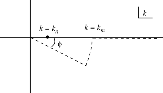
FIG. 1.: The rotated contour of integration. Here $k_{0}$ is the on-shell momentum

FIG. 2.: The behaviour of the inverse of the bare coupling $\lambda$ as a function of $1/\epsilon$, as obtained using the dimensionally-regularized Lippmann-Schwinger equation

FIG. 3.: Phase shifts at E${}_{\rm Lab}=24.0$ MeV for the solution of the LS equation as a function of $\epsilon$ for $\epsilon\rightarrow 0$.

FIG. 4.: Phase shifts at E${}_{\rm Lab}=352.0$ MeV for the solution of the LS equation as a function of $\epsilon$ for $\epsilon\rightarrow 0$.

FIG. 5.: Phase shifts at E${}_{\rm Lab}=352.0$ MeV with $\epsilon=6.1035\times 10^{-5}$, for the solution of the LS equation as a function of $k_{m}$.