FZJ-IKP(TH)-1999-10
MKPH-98-11
Generalized Polarizabilities of the Nucleon in Chiral Effective Theories

Abstract

Using the techniques of chiral effective field theories we evaluate the so called “generalized polarizabilities”, which characterize the structure dependent components in virtual Compton scattering (VCS) off the nucleon as probed in the electron scattering reaction $eN\rightarrow e^{\prime}N\gamma$. Results are given for both spin-dependent and spin-independent structure effects to ${\cal O}(p^{3})$ in SU(2) Heavy Baryon Chiral Perturbation Theory and to ${\cal O}(\epsilon^{3})$ in the SU(2) “Small Scale Expansion”.

I Introduction

One of the primary goals of contemporary particle/nuclear physics is to understand the structure of the nucleon. Indeed this is being pursued at the very highest energy machines such as HERA and SLAC, at which one probes the quark/parton substructure, as well as at lower energy accelerators such as BATES, ELSA and MAMI, wherein one studies the low energy structure of the nucleon via electron scattering. In recent years another important low energy probe has been (real) Compton scattering, by which one can study the deformation of the nucleon under the influence of quasi-static electric and/or magnetic fields [1]. For example, in the presence of an external electric field $\vec{E}$ the quark distribution of the nucleon becomes distorted, leading to an induced electric dipole moment

$$\vec{p}=4\pi\alpha_{E}\vec{E}$$ (1)

in the direction of the applied field, where $\alpha_{E}$ is the electric polarizability. The interaction of this dipole moment with the field leads to a corresponding interaction energy

$$U=-{1\over 2}4\pi\alpha_{E}\vec{E}^{2}.$$ (2)

Similarly in the presence of an applied magnetizing field $\vec{H}$ there will be an induced magnetic dipole moment

$$\vec{\mu}=4\pi\beta_{M}\vec{H}$$ (3)

and an interaction energy

$$U=-{1\over 2}4\pi\beta_{M}\vec{H}^{2}.$$ (4)

For wavelengths large compared to the size of the system, the effective Hamiltonian for the interaction of a system of charge $e$ and mass $m$ with an electromagnetic field is, of course, given by the simple form

$$H^{(0)}={(\vec{p}-e\vec{A})^{2}\over 2m}+e\phi,$$ (5)

and the Compton scattering cross section has simply the familiar Thomson form

$${d\sigma\over d\Omega}=\left({\alpha_{em}\over m}\right)^{2}\left({\omega^{\prime}\over\omega}\right)^{2}[{1\over 2}(1+\cos^{2}\theta)],$$ (6)

where $\alpha_{em}$ is the fine structure constant and $\omega,\omega^{\prime}$ are the initial, final photon energies respectively. As the energy increases, however, so does the resolution and one must take into account also polarizability effects, whereby the effective Hamiltonian becomes

$$H_{\rm eff}=H^{(0)}-{1\over 2}4\pi(\alpha_{E}\vec{E}^{2}+\beta_{M}\vec{H}^{2}).$$ (7)

The Compton scattering cross section from such a system (taken, for simplicity, to be spinless) is given then by

$${d\sigma\over d\Omega} = \left({\alpha_{em}\over m}\right)^{2}\left({\omega^{\prime}\over\omega}\right)^{2}[{1\over 2}(1+\cos^{2}\theta)$$ (8)

$$- {m\omega\omega^{\prime}\over\alpha_{em}}[{1\over 2}(\alpha_{E}+\beta_{M})(1+\cos\theta)^{2}+{1\over 2}(\alpha_{E}-\beta_{M})(1-\cos\theta)^{2}+\ldots].$$ (9)

It is clear from Eq.(9) that from careful measurement of the differential scattering cross section, extraction of these structure dependent polarizability terms is possible provided that i) the energy is large enough that these terms are significant compared to the leading Thomson piece and ii) that the energy is not so large that higher order corrections become important. In this way the measurement of electric and magnetic polarizabilities for the proton has recently been accomplished using photons in the energy range 50 MeV $<\omega<$ 100 MeV, yielding[2]

$$\alpha_{E}^{p} = (12.1\pm 0.8\pm 0.5)\times 10^{-4}\;{\rm fm}^{3}$$ (10)

$$\beta_{M}^{p} = (2.1\mp 0.8\mp 0.5)\times 10^{-4}\;{\rm fm}^{3}.$$ (11)

Note that in practice one generally exploits the strictures of causality and unitarity as manifested in the validity of the forward scattering dispersion relation, which yields the Baldin sum rule[6]

$$\alpha_{E}^{p,n}+\beta_{M}^{p,n}={1\over 2\pi^{2}}\int_{0}^{\infty}{d\omega\over\omega^{2}}\sigma_{\rm tot}^{p,n}=\left\{\begin{array}[]{ll}(13.69\pm 0.14)\times 10^{-4}{\rm fm}^{3}&{\rm proton}\\ (14.40\pm 0.66)\times 10^{-4}{\rm fm}^{3}&{\rm neutron}\end{array}\right.$$ (12)

as a rather precise constraint because of the small uncertainty associated with the photoabsorption cross section $\sigma_{\rm tot}^{p}$.

From these results, which imply that the polarizabilities of the proton are nearly a factor of a thousand smaller than its volume, we learn that the nucleon is a relatively rigid object when compared to the hydrogen atom, for example, for which the electric polarizability and volume are comparable.

Additional probes of proton structure are possible if one exploits its spin $\vec{S}$. Thus, for example, the presence of a time varying electric field in the plane of a rotating system of charges will lead to a charge separation with induced electric dipole moment

$$\vec{p}=-\gamma_{1}\vec{S}\times{\partial\vec{E}\over\partial t}$$ (13)

and corresponding interaction energy

$$U_{1}=-\vec{p}\cdot\vec{E}=\gamma_{1}\vec{E}\cdot\vec{S}\times(\vec{\nabla}\times\vec{B}),$$ (14)

where we have used the Maxwell equations in writing this form. This is a quantum mechanical analog of the familiar Faraday rotation. (Note that the ”extra” time or spatial derivative is required by time reversal invariance since $\vec{S}$ is T-odd.) Similarly other possible structures are[7, 8]

$$U_{2} = \gamma_{2}\vec{B}\cdot\vec{\nabla}\vec{S}\cdot\vec{E}$$ (15)

$$U_{3} = \gamma_{3}\vec{E}\cdot\vec{\nabla}\vec{S}\cdot\vec{B}$$ (16)

$$U_{4} = \gamma_{4}\vec{B}\cdot\vec{S}\times(\vec{\nabla}\times\vec{E}),$$ (17)

and the measurement of these various ”spin-polarizabilities” $\gamma_{i}$ via polarized Compton scattering provides a rather different probe for nucleon structure. Because of the requirement for polarization not much is known at present about such spin-polarizabilities, although from dispersion relations the combination

$$\gamma_{0}^{p}\equiv\gamma_{1}^{p}-\gamma_{2}^{p}-2\gamma_{4}^{p}\approx\left\{\begin{array}[]{cc}-1.34\times 10^{-4}\;{\rm fm}^{4}&{\rm SAID}\cite[cite]{[\@@bibref{Number}{DHS}{}{}]}\\ -0.80\times 10^{-4}\;{\rm fm}^{4}&{\rm Mainz}\cite[cite]{[\@@bibref{Number}{HDT}{}{}]}\end{array}\right.$$ (18)

has been evaluated and from a global analysis of unpolarized Compton data, to which it contributes at ${\cal O}(\omega^{4})$, Tonnison et al.[10] have determined the so-called backward spin-polarizability to be

$$\gamma_{\pi}=\gamma_{1}+\gamma_{2}+2\gamma_{4}=(27.7\pm 2.3\pm 2.5)\times 10^{-4}\;{\rm fm}^{4}.$$ (19)

Clearly such measurements represent an important goal for the future.

At the same time it has come to be realized that a high resolution probe of nucleon structure is available, in principle, via the use of virtual Compton scattering—VCS—wherein virtual photons produced from scattered electrons are scattered off a nucleon into real final state photons, transferring a three-momentum $\bar{q}$ to the target. The outcome of such measurements is, in principle, $\bar{q}$-dependent values of the polarizabilities (usually termed ”generalized polarizabilities” and denoted by GPs in the following) which can be thought of as the Fourier transforms of local polarization densities in the nucleon. At the present time a VCS experiment has already taken place at MAMI, and there exist approved experiments at BATES and TJNAF. Preliminary results have been reported from MAMI and will be discussed in the conclusion [12]. It is therefore appropriate to have a base of solid theoretical predictions with which such data can be confronted. The here presented approach, which utilizes the techniques of chiral effective theories in the heavy fermion formulation, has already yielded several results[13, 14]. In the first chiral calculation of generalized polarizabilities utilizing SU(2) Heavy Baryon Chiral Perturbation Theory (HBChPT) [13], the leading momentum-dependent modification of the (generalized) electric ($\bar{\alpha}_{E}(\bar{q})$) and magnetic ($\bar{\beta}_{M}(\bar{q})$) polarizabilities was analyzed. Later, in a short communication[14], numerical studies for the full $\bar{q}$-dependence of all 10 generalized (Guichon) polarizabilities were presented—again using the framework of SU(2) HBChPT. In this work we present the details behind the numerical study of ref.[14] and, for the first time in the field of VCS, are able to present simple analytical expressions for all GPs in a momentum range from $0<\bar{q}^{2}<0.5$ GeV² utilizing SU(2) HBChPT. These new expressions greatly facilitate the study of the influence of the chiral “pion cloud” on the GPs and the comparison with model calculations. Furthermore, we also investigate the leading modifications of the GPs’ $\bar{q}$-dependence due to $\Delta$(1232) resonance contributions utilizing a different effective chiral lagrangian approach—the so called “small scale expansion” (SSE) [15]. SSE results have already been reported for real Compton scattering [16, 17], and in the present work we generalize the analysis to the VCS case.

In the next section we shall discuss the definition of the generalized polarizabilities, while in Section III we present an introduction to the way in which our heavy baryon calculations—valid to one loop—are carried out. In section IV we show how to connect our predictions to the general formulation of VCS and how to extract the desired generalized polarizabilities. In section V, we present the results of our calculations. Finally, we summarize our findings in a concluding section VI.

II Generalized Polarizabilities

Recently a new frontier in Compton scattering has been opened (see, e.g., [18]) and is now in the beginning of being explored: the study of the electron scattering process $ep\rightarrow e^{\prime}p^{\prime}\gamma$ (cf. Fig. 1) in order to obtain information concerning the virtual Compton scattering (VCS) process $\gamma^{*}N\rightarrow\gamma N$. As will be discussed below, in addition to the two kinematical variables of real Compton scattering— the scattering angle $\theta$ and the energy $\omega^{\prime}$ of the outgoing photon—the invariant structure functions for VCS [20, 21] depend on a third kinematical variable, e.g. the magnitude of the three–momentum transfer to the nucleon in the hadronic c.m. frame, $\bar{q}\equiv|\vec{q}|$. As shown in ref. [21], the VCS amplitude can then be characterized in terms of $\bar{q}$-dependent GPs, in analogy to the well-known polarizability coefficients in real Compton scattering. However, due to the specific kinematic approximation chosen in [21] there does not exist a one–to–one correspondence between the real Compton polarizabilities and the GPs of Guichon et al. in VCS[21, 22, 23].

The advantage of VCS lies in the virtual nature of the initial state photon and the associated possibility of an independent variation of photon energy and momentum, thus rendering access to a much greater variety of structure information than in the case of real Compton scattering. For example, one can hope to identify individual signatures of specific nucleon resonances which cannot be obtained in other processes[18]. In this regard, it should be noted that a great deal of theoretical work already exists, such as predictions within a non–relativistic constituent quark model[21], a one–loop calculation in the linear sigma model[24], a Born term model including nucleon resonance effects[25], a HBChPT calculation of the leading $\bar{q}$-dependence of the generalized electric and magnetic polarizability [13], a calculation of $\bar{\alpha}_{E}(\bar{q}^{2})$ in the Skyrme model[26] and the numerical study of all 10 GPs again utilizing HBChPT [14]. For an overview of the status at higher energies and in the deep inelastic regime we refer to [18].

The GPs of the nucleon have been defined by Guichon et al. in terms of electromagnetic multipoles as functions of the initial photon momentum $\bar{q}$[21],

$$P^{(\rho^{\prime}L^{\prime},\rho L)S}(\bar{q}^{2}) = \left[\frac{1}{\omega^{\prime L}\bar{q}^{L}}H^{(\rho^{\prime}L^{\prime},\rho L)S}(\omega^{\prime},\bar{q})\right]_{\omega^{\prime}=0}\,,$$ (20)

$$\hat{P}^{(\rho^{\prime}L^{\prime},L)S}(\bar{q}^{2}) = \left[\frac{1}{\omega^{\prime L}\bar{q}^{L+1}}\hat{H}^{(\rho^{\prime}L^{\prime},L)S}(\omega^{\prime},\bar{q})\right]_{\omega^{\prime}=0}\,,$$ (21)

where $L$ ($L^{\prime}$) denotes the initial (final) photon angular momentum, $\rho$ ($\rho^{\prime}$) the type of multipole transition ($0=C$ (scalar, Coulomb), $1=M$ (magnetic), $2=E$ (electric)), and $S$ distinguishes between non–spin–flip ($S=0$) and spin–flip ($S=1$) transitions. In addition, mixed–type polarizabilities, ${\hat{P}}^{(\rho^{\prime}L^{\prime},L)S}(\bar{q}^{2})$, have been introduced, which are neither purely electric nor purely Coulomb type. It is important to note that the above definitions are based on the kinematical approximation that the multipoles are expanded around $\omega^{\prime}=0$ and only terms linear in $\omega^{\prime}$ are retained, which, together with current conservation, yields selection rules for the possible combinations of quantum numbers of the GPs. In this approximation, 10 GPs have been introduced in [21] as functions of $\bar{q}^{2}$: $P^{(01,01)0}$, $P^{(11,11)0}\,$, $P^{(01,01)1}\,$, $P^{(11,11)1}\,$, $P^{(01,12)1}\,$, $P^{(11,02)1}\,$, $P^{(11,00)1}\,$, ${\hat{P}}^{(01,1)0}\,$, ${\hat{P}}^{(01,1)1}\,$, ${\hat{P}}^{(11,2)1}\,$.

However, recently it has been proven[22, 23], using crossing symmetry and charge conjugation invariance, that only six of the above ten GPs are independent. With

$$\omega_{0}\equiv M_{N}-\sqrt{M_{N}^{2}+\bar{q}^{2}}=-\;\frac{\bar{q}^{2}}{2M_{N}}+{\cal O}(1/M_{N}^{3})$$ (22)

and $M_{N}$ being the nucleon mass, the four constraints implied by $C$ invariance and crossing can be written as

$$0 = \sqrt{\frac{3}{2}}P^{(01,01)0}(\bar{q}^{2})+\sqrt{\frac{3}{8}}P^{(11,11)0}(\bar{q}^{2})+\frac{3\bar{q}^{2}}{2\omega_{0}}\hat{P}^{(01,1)0}(\bar{q}^{2})\,,$$ (23)

$$0 = P^{(11,11)1}(\bar{q}^{2})+\sqrt{\frac{3}{2}}\omega_{0}P^{(11,02)1}(\bar{q}^{2})+\sqrt{\frac{5}{2}}\bar{q}^{2}\hat{P}^{(11,2)1}(\bar{q}^{2})\,,$$ (24)

$$0 = 2\omega_{0}P^{(01,01)1}(\bar{q}^{2})+2\frac{\bar{q}^{2}}{\omega_{0}}P^{(11,11)1}(\bar{q}^{2})-\sqrt{2}\bar{q}^{2}P^{(01,12)1}(\bar{q}^{2})+\sqrt{6}\bar{q}^{2}\hat{P}^{(01,1)1}(\bar{q}^{2})\,,$$ (25)

$$0 = 3\frac{\bar{q}^{2}}{\omega_{0}}P^{(01,01)1}(\bar{q}^{2})-\sqrt{3}P^{(11,00)1}(\bar{q}^{2})-\sqrt{\frac{3}{2}}\bar{q}^{2}P^{(11,02)1}(\bar{q}^{2})\,.$$ (26)

In the scalar (i.e. spin–independent) sector the first of Eqs.(26) allows us to eliminate the mixed polarizability ${\hat{P}}^{(01,1)0}$ in favor of $P^{(01,01)0}$ and $P^{(11,11)0}$, which are simply generalizations of the familiar electric and magnetic polarizabilities in real Compton scattering

$$\bar{\alpha}_{E}(\bar{q}^{2}) = -\frac{e^{2}}{4\pi}\sqrt{\frac{3}{2}}P^{(01,01)0}(\bar{q}^{2})\,,$$ (27)

$$\bar{\beta}_{M}(\bar{q}^{2}) = -\frac{e^{2}}{4\pi}\sqrt{\frac{3}{8}}P^{(11,11)0}(\bar{q}^{2})\,.$$ (28)

In the limit $\bar{q}\rightarrow 0$ they reduce to the real Compton polarizabilities $\bar{\alpha}_{E},\,\bar{\beta}_{M}$ of Eq.(11).

In the spin-dependent sector it is not a priori clear which three of the seven GPs $P^{(01,01)1}\,$, $P^{(11,11)1}\,$, $P^{(01,12)1}\,$, $P^{(11,02)1}\,$, $P^{(11,00)1}\,$, ${\hat{P}}^{(01,1)1}\,$, ${\hat{P}}^{(11,2)1}\,$. should be eliminated by use of Eq.(26). However, the chiral analysis performed here shows that to leading order only 4 of the 7 spin GPs can be calculated—$P^{(01,12)1},\,P^{(11,02)1},\,P^{(11,00)1},\,{\hat{P}}^{(01,1)1}$. Naturally we focus on these four spin GPs, as $P^{(01,01)1},\,P^{(11,11)1},\,{\hat{P}}^{(11,2)1}$ possess an extra suppression factor of $1/M_{N}$ (see section V A 3) which pushes them outside the validitiy of our analysis. Still, one can reconstruct the whole set of spin GPs via Eq.(26) if one wishes to do so. Finally, we note that in the spin-sector one can also establish a (partial) connection between the GPs defined in the context of VCS by Guichon et al. [21] and the 4 real Compton spin polarizabilities $\gamma_{i},\;i=1...4$ of Ragusa [7] given in Eqs.(14) and (15):

$$\gamma_{3} = -\frac{e^{2}}{4\pi}\,\frac{3}{\sqrt{2}}\,P^{(01,12)1}(\bar{q}\rightarrow 0)$$ (29)

$$\gamma_{2}+\gamma_{4} = -\frac{e^{2}}{4\pi}\,\frac{3\sqrt{3}}{2\sqrt{2}}\,P^{(11,02)1}(\bar{q}\rightarrow 0)$$ (30)

These model-independent relations might provide an interesting possibility to determine some of the elusive (Ragusa) spin-polarizabilities by the upcoming experiments.

III The chiral framework

A Pion-Nucleon ChPT

We want to perform the VCS calculation to ${\cal O}(p^{3})$ in Heavy Baryon Chiral Perturbation Theory (HBChPT) (e.g. see [27]). We therefore need the lagrangians

$${\cal L}_{VCS}^{(3)}={\cal L}_{N}^{(3)}+{\cal L}_{\pi}^{(4)}.$$ (31)

We begin our discussion in the nucleon sector. For VCS to ${\cal O}(p^{3})$ we need the lagrangians

$${\cal{L}}_{N}^{(3)}={\cal{L}}_{\pi N}^{(1)}+{\cal{L}}_{\pi N}^{(2)}+{\cal{L}}_{\pi N}^{(3)}\,,$$ (32)

with

$${\cal{L}}_{\pi N}^{(1)} = \bar{N}_{v}(iv\cdot D+\dot{g}_{A}S\cdot u)N_{v}\,,$$ (33)

$${\cal{L}}_{\pi N}^{(2)} = \frac{1}{2M_{0}}\bar{N}_{v}\left\{(v\cdot D)^{2}-D^{2}-\frac{i}{2}\left[S^{\mu},S^{\nu}\right]\left[\left(1+\dot{\kappa}_{v}\right)f_{\mu\nu}^{+}+2\left(1+\dot{\kappa}_{s}\right)v_{\mu\nu}^{(s)}\right]+\dots\right\}N_{v}\;,$$ (34)

$${\cal{L}}_{\pi N}^{(3)} = \frac{-1}{8M_{0}^{2}}\bar{N}_{v}\left\{\left(1+2\dot{\kappa}_{v}\right)\left[S_{\mu},S_{\nu}\right]f_{+}^{\mu\sigma}v_{\sigma}D^{\nu}+2\left(\dot{\kappa}_{s}-\dot{\kappa}_{v}\right)\left[S_{\mu},S_{\nu}\right]v_{(s)}^{\mu\sigma}v_{\sigma}D^{\nu}+\mathrm{h.c.}+\dots\right\}N_{v}\;,$$ (35)

where we have only kept those terms which contribute to our VCS calculation. Furthermore, all terms which vanish in the “Coulomb gauge” $v\cdot A=0$, with $v_{\mu}$ being the velocity vector $(v^{2}=1)$ of the nucleon and $A_{\mu}$ denoting a photon field, have been omitted. The velocity-dependent nucleon field $N_{v}$ is projected from the relativistic nucleon Dirac field $\Psi_{N}$ via

$$N_{v}={\rm{exp}}\left[iM_{0}v\cdot x\right]P_{v}^{+}\Psi_{N}\,,$$ (36)

where the velocity projection operator is given by

$$P_{v}^{+}=\frac{1}{2}\left(1+\not\!{v}\right)\,.$$ (37)

$S_{\mu}$ denotes the usual Pauli-Lubanski vector (e.g. [27]) and $D_{\mu}$ corresponds to the covariant derivative of the nucleon

$$D_{\mu}\,N_{v}=\left[\partial_{\mu}+\Gamma_{\mu}-iv_{\mu}^{(s)}\right]N_{v}.$$ (38)

One also encounters the following chiral tensors in the VCS calculation:

$$U = u^{2}={\mathrm{exp}}\left(i\vec{\tau}\cdot\vec{\pi}/F_{\pi}\right)$$ (39)

$$\Gamma_{\mu} = \frac{1}{2}\left\{u^{\dagger}\left(\partial_{\mu}-i\,e\,\frac{\tau^{3}}{2}\,A_{\mu}\right)u+u\left(\partial_{\mu}-i\,e\,\frac{\tau^{3}}{2}\,A_{\mu}\right)u^{\dagger}\right\}\;,$$ (40)

$$u_{\mu} = i\left\{u^{\dagger}\left(\partial_{\mu}-i\,e\,\frac{\tau^{3}}{2}\,A_{\mu}\right)u-u\left(\partial_{\mu}-i\,e\,\frac{\tau^{3}}{2}\,A_{\mu}\right)u^{\dagger}\right\}\;.$$ (41)

In Eq.(41) $\vec{\tau}$ are the conventional Pauli isospin matrices, while $\vec{\pi}$ represents the interpolating pion field. Furthermore, $v_{\mu}^{(s)}=e\,\frac{1}{2}\,A_{\mu}$ denotes an isoscalar photon field and the corresponding field strength tensors in Eq.(35) are defined as

$$v_{\mu\nu}^{(s)} = \partial_{\mu}v_{\nu}^{(s)}-\partial_{\nu}v_{\mu}^{(s)}\,,$$ (42)

$$f_{+}^{\mu\nu} = u\,e\frac{\tau^{3}}{2}\,\left(\partial_{\mu}A_{\nu}-\partial_{\nu}A_{\mu}\right)u^{\dagger}+u^{\dagger}\,e\frac{\tau^{3}}{2}\,\left(\partial_{\mu}A_{\nu}-\partial_{\nu}A_{\mu}\right)u\,.$$ (43)

From the pion sector we require information up to ${\cal O}(p^{4})$ for a ${\cal O}(p^{3})$ VCS calculation. Utilizing “standard ChPT” [29] (i.e. the assumption of a “large” quark condensate parameter $B$) one finds

$${\cal L}_{\pi}^{(4)}={\cal L}_{\pi\pi}^{(2)}+{\cal L}_{\pi\pi}^{(4)}$$ (44)

with

$${\cal{L}}_{\pi\pi}^{(2)} = \frac{F_{0}^{2}}{4}{\mathrm{tr}}\left[\left(\nabla_{\mu}U\right)^{\dagger}\nabla^{\mu}U+\chi^{\dagger}U+\chi U^{\dagger}\right]\;,$$ (45)

$${\cal{L}}_{\pi\pi}^{(4)} = {e^{2}\over 32\pi^{2}F_{0}}\epsilon^{\mu\nu\alpha\beta}F_{\mu\nu}F_{\alpha\beta}\pi^{0}+\ldots\;,$$ (46)

where again we have omitted all terms not required for the VCS calculation. Note that the only piece shown from the chiral ${\cal O}(p^{4})$ meson lagrangian is the so called “anomalous” or “Wess-Zumino” term [30], which one needs for the ${\cal O}(p^{3})$ pion-pole diagram of VCS shown in Fig.3(f). In the lagrangians of Eq.(45) one also encounters the chiral tensors

$$\nabla_{\mu}U = \partial_{\mu}U-i\,\frac{e}{2}\,A_{\mu}\left[\tau_{3},U\right]\;,$$ (47)

$$\chi = 2\,B\,{\it M}\;,$$ (48)

where ${\it M}$ denotes the SU(2) quark mass matrix in the isospin limit $m_{u}=m_{d}$.

Finally, we emphasize that we do not require any additional diagrams compared to the ${\cal O}(p^{3})$ calculation for real Compton scattering [31]. The complete set of non-zero diagrams we have to calculate is given in Fig.3 ((a) $s$-channel, (b) $u$-channel, (c) contact diagram and (f) $t$-channel pole term) and Fig.4 ($N\pi$-loop diagrams). In the following we will treat the tree and loop parts of the amplitudes separately,

$$A_{i}=A_{i}^{tree}+A_{i}^{loop}\,,$$ (49)

since the generalized polarizabilities are contained only in the latter.

B $\Delta$(1232) and the Small Scale Expansion

In standard SU(2) HBChPT, nucleon resonances like the $\Delta$(1232) are considered to be much heavier than the nucleon and therefore only contribute via local counterterms. This approach is particularly well-suited for near-threshold processes (e.g. the multipole $E_{0+}$ in threshold pion photoproduction) where the resonance contributions are small and their contribution to counterterms can be estimated by a simple Born diagram analysis. However, if one wants to move away from threshold, nucleon resonances, in particular the lowest lying SU(2) resonance $\Delta$(1232), contribute as dynamical degrees of freedom and the theoretical treatment in terms of local counterterms generates a slowly converging perturbative series. In this kinematical regime it is therefore advantageous to formulate an effective field theory which keeps the resonance as an explicit degree of freedom. In addition to this dynamical consideration there is also another practical concern regarding the inclusion of resonance effects via counterterms. Even if simple Born exchange might be the dominant contribution of a particular resonance, the local counterterm in the chiral Lagrangian that subsumes this effect might be of higher order in the calculation, so that the leading and even the subleading result can misrepresent the perturbative series. A well-known example of this type are the so-called spin-polarizabilities of the nucleon, wherein one encounters very large contributions due to $\Delta$(1232) Born graphs that only start contributing via counterterms at ${\cal O}(p^{5})$ in the chiral calculation (e.g. [17]). Situations of this type require a “resummation” of the standard chiral expansion in order to push resonance effects into lower orders to restore meaningful perturbative expansions for quantities of interest in low energy baryon physics.

In order to address these two different but related issues in the field of resonance physics in baryon CHPT, the so called “small scale expansion” of SU(2) baryon ChPT has recently been formulated [15, 32]. In this chiral effective theory one treats the nucleon and the first nucleon resonance—$\Delta$(1232)—as explicit degrees of freedom, and, to address the second problem, the chiral power counting is modified to bring $\Delta$(1232) related effects into lower orders of the calculation. In the “small scale expansion” one organizes the Lagrangian and the calculation in powers of the scale ”$\epsilon$”, which, in addition to the chiral expansion parameters of small momenta $q$ and the pion mass $m_{\pi}$, also includes the $\Delta(1232)-N(940)$ mass splitting $\Delta=M_{\Delta}-M_{N}$. Of course, this modification of the chiral counting implies that one has to repeat the whole procedure of construction of the Lagrangian and the determination of counterterms and coupling constants, even for processes which only involve nucleons in the initial and final states. For first results regarding the modified renormalization of nucleon parameters we refer to [28].

For our calculation below, which (as far as the GPs are concerned) is done only to leading order—${\cal O}(\epsilon^{3})$—in the small scale expansion of the (generalized) polarizabilities, we shall require only the propagator involving the $\Delta(1232)$ as well as the couplings $NN\gamma$, $NN\gamma\gamma$, $N\Delta\pi$ and $N\Delta\gamma$. Details of the “small scale expansion” formalism are given in ref. [32]. Here we only list the minimal structures necessary for the present calculation. The systematic 1/M-expansion of the coupled $N\Delta$-system starts with the most general relativistic chiral invariant lagrangian involving spin 1/2 ($\psi_{N}$) and spin 3/2 ($\psi^{i}_{\mu}$) baryon fields. The “light” spin 3/2 field $T^{i}_{\mu}$ in the effective low-energy theory is projected from its relativistic Rarita-Schwinger counterpart $\psi^{i}_{\mu}$ via

$$T_{\mu}^{i}(x)\equiv P_{v}^{+}\;P^{3/2}_{(33)\mu\nu}\;\psi^{\nu}_{i}(x)\;\mbox{exp}(iM_{0}v\cdot x),$$ (50)

where we have introduced a spin 3/2 projection operator for fields with fixed velocity $v_{\mu}$

$$P^{3/2}_{(33)\mu\nu}=g_{\mu\nu}-\frac{1}{3}\gamma_{\mu}\gamma_{\nu}-\frac{1}{3}\left(\not\!{v}\gamma_{\mu}v_{\nu}+v_{\mu}\gamma_{\nu}\not\!{v}\right).$$ (51)

The remaining components,

$$G_{\mu}^{i}(x)=\left(g_{\mu\nu}-P_{v}^{+}\;P^{3/2}_{(33)\mu\nu}\right)\psi^{\nu}_{i}(x)\;\mbox{exp}(iM_{0}v\cdot x),$$ (52)

can be shown to be “heavy” [32] and are integrated out. Resulting from this procedure one finds the (non-relativistic) chiral lagrangians of the “small scale expansion” (SSE):

$${\cal L}^{SSE}={\cal L}_{N}^{SSE}+{\cal L}_{\Delta}^{SSE}+\left({\cal L}_{N\Delta}^{SSE}+h.c.\right).$$ (53)

To the order we are working here ${\cal L}_{N}^{SSE}$ agrees with the chiral lagrangian ${\cal L}_{N}^{(3)}$ (Eq.(32)) needed for VCS. From the chiral SSE lagrangians explicitly involving the $\Delta$ field we need the structures [32]

$${\cal L}^{(1)}_{\Delta} = -\bar{T}^{\mu}_{i}g_{\mu\nu}\left[iv\cdot D^{ij}-\Delta_{0}\;\delta^{ij}+\ldots\right]T^{\nu}_{j}$$ (54)

$${\cal L}^{(1)}_{N\Delta} = g_{\pi N\Delta}\bar{T}^{\mu}_{i}\;w_{\mu}^{i}\;N+{\rm h.c.}$$ (55)

$${\cal L}^{(2)}_{N\Delta} = \bar{T}^{\mu}_{i}\left[{ib_{1}\over M_{0}}\;S^{\nu}\;f_{+\mu\nu}^{i}+\ldots\right]N+{\rm h.c.},$$ (56)

where $\Delta_{0}=M_{\Delta}-M_{0}$ can be identified with the physical delta-nucleon mass difference to the order we are working, i.e. $M_{0}\equiv M_{N}$. The corresponding chiral tensors needed for VCS read

$$D_{\mu}^{ij} = \partial_{\mu}\delta^{ij}-i\frac{e}{2}\left(1+\tau_{3}\right)A_{\mu}\delta^{ij}+e\epsilon^{i3j}A_{\mu}+\ldots$$ (57)

$$w_{\mu}^{i} = -\frac{1}{F_{\pi}}\partial_{\mu}\pi^{i}-\frac{e}{F_{\pi}}A_{\mu}\epsilon^{i3j}\pi^{j}+\ldots$$ (58)

$$f_{+\mu\nu}^{i} = e\delta^{i3}\left(\partial_{\mu}A_{\nu}-\partial_{\nu}A_{\mu}\right)+\dots$$ (59)

The coupling constants defined in Eq.(56) are determined from fits to the strong and electromagnetic decay widths of the Delta resonance within the “small scale expansion”. To the order we are working one requires [17, 33] $g_{\pi N\Delta}=1.05\pm 0.02$ and $b_{1}=3.85\pm 0.15$.

The leading propagator for a $\Delta$(1232) field with small momentum $k_{\mu}$ is then given by

$$S^{3/2}_{\mu\nu}={-iP^{3/2}_{\mu\nu}\over v\cdot k-\Delta+i\eta}\xi^{ij}_{I=3/2},$$ (60)

where $P^{3/2}_{\mu\nu}$ is the spin-${3\over 2}$ heavy baryon projector in d-dimensions [32]

$$P^{3/2}_{\mu\nu}=g_{\mu\nu}-v_{\mu}v_{\nu}+{4\over d-1}S_{\mu}S_{\nu},$$ (61)

and

$$\xi^{ij}_{I=3/2}=\delta^{ij}-{1\over 3}\tau^{i}\tau^{j}$$ (62)

is the corresponding isospin projector. The vertices relevant for our calculation can be read off directly from Eq.(56). As in the nucleon case, the resulting diagrams can be separated into two classes—one-loop graphs and Born graphs. The systematics of the “small scale expansion” uniquely fixes the number and type of diagrams for VCS to be calculated to ${\cal O}(\epsilon^{3})$. It turns out that to the order we are working there are two Born diagrams involving the $\Delta$(1232) (Fig.3(d,e)) and nine $\Delta\pi$-loop diagrams (Fig.5), which turn out to have exactly the same structure as their chiral $N\pi$ analogues (cf. Fig.4). However, before undertaking any such calculation, it is necessary to work out the formalism for VCS.

IV Virtual Compton Scattering

A General Structure

We begin by specifying our notation for the virtual Compton process

$$\gamma^{*}(\epsilon^{\mu},q^{\mu})+N(p_{i}^{\mu})\rightarrow\gamma(\epsilon^{\prime*\mu},q^{\prime\mu})+N(p_{f}^{\mu}).$$ (63)

Here the nucleon four-momenta in the initial and final states are denoted by $p_{i}^{\mu}=(E_{i},\vec{p}_{i})$ and $p_{f}^{\mu}=(E_{f},\vec{p}_{f})$ respectively. The virtual initial [real final] state photon is characterized by its four-momentum $q^{\mu}=(\omega,\vec{q}),\;q^{2}<0$ [$q^{\prime\mu}=(\omega^{\prime},\vec{q}^{\;\prime}),\;q^{\prime 2}=0$] and polarization vector $\epsilon^{\mu}=(\epsilon_{0},\vec{\epsilon})$ [$\epsilon^{\prime\mu}=(\epsilon^{\prime}_{0},\vec{\epsilon}^{\;\prime})$].

Since our discussion refers to an electron scattering experiment, wherein the virtual photon is exchanged between the electron and hadron currents, the polarization vector of the incoming photon is given by

$$\epsilon_{\mu}=e\;\bar{u}_{e^{\prime}}(k_{1})\;\gamma_{\mu}\;u_{e}(k_{2})\;\frac{1}{q^{2}}\;,$$ (64)

where $u_{e}(k_{1}),\bar{u}_{e^{\prime}}(k_{2})$ are electron Dirac spinors with four-momenta $k_{1}^{\mu}\;(k_{2}^{\mu})$ before (after) emission of the virtual photon. The unit charge $e$ is taken as $e=\sqrt{4\pi/137}>0$.

In addition to the proper VCS process displayed in Fig.2a there are also Bethe-Heitler processes taking place (Fig.2b,c),

$${\cal M}_{eN\rightarrow e^{\prime}N\gamma}={\cal M}^{VCS}+{\cal M}^{Bethe-Heitler},$$ (65)

and such Bethe-Heitler contributions must be carefully evaluated before one can infer any information about the VCS matrix element from the electron scattering cross section. In the following, however, we will focus on the evaluation of the VCS matrix element ${\cal M}^{VCS}$ (Fig.2a). For details on ${\cal M}^{Bethe-Heitler}$ and the calculation of the cross section we refer to [12] and references therein.

From now on we will work in the center of mass system of the final state photon-nucleon subsystem,

$$\vec{p}_{f}=-\vec{q}^{\;\prime}, \vec{p}_{i}=-\vec{q}=-\bar{q}\;\hat{e}_{z}\;,$$ (66)

$$\omega^{\prime}+\sqrt{M_{N}^{2}+\omega^{\prime 2}} = \omega+\sqrt{M_{N}^{2}+\bar{q}^{2}}\;,$$ (67)

where the $z$-axis is defined by the three-momentum vector $\vec{q}$ of the incoming virtual photon. Utilizing the Lorentz gauge,

$$\epsilon\cdot q=0,\qquad\epsilon_{0}=\frac{\bar{q}}{\omega}\;\epsilon_{z}\;,$$ (68)

with $\vec{\epsilon}=\vec{\epsilon}_{T}+\epsilon_{z}\hat{e}_{z}$, one can express the VCS matrix element in terms of twelve independent kinematic forms

$${\cal M}^{VCS} = i\;e^{2}\left\{\vec{\epsilon}^{\;\prime*}\cdot\vec{\epsilon}_{T}\;A_{1}+\vec{\epsilon}^{\;\prime*}\cdot\hat{q}\;\vec{\epsilon}_{T}\cdot\hat{q}^{\prime}\;A_{2}+i\vec{\sigma}\cdot\left(\vec{\epsilon}^{\;\prime*}\times\vec{\epsilon}_{T}\right)A_{3}+i\;\vec{\sigma}\cdot\left(\hat{q}^{\prime}\times\hat{q}\right)\vec{\epsilon}^{\;\prime*}\cdot\vec{\epsilon}_{T}\;A_{4}\right.$$ (72)

$$\phantom{i\;e^{2}}+i\;\vec{\sigma}\cdot\left(\vec{\epsilon}^{\;\prime*}\times\hat{q}\right)\vec{\epsilon}_{T}\cdot\hat{q}^{\prime}\;A_{5}+i\;\vec{\sigma}\cdot\left(\vec{\epsilon}^{\;\prime*}\times\hat{q}^{\prime}\right)\vec{\epsilon}_{T}\cdot\hat{q}^{\prime}\;A_{6}$$

$$\phantom{i\;e^{2}}-i\;\vec{\sigma}\cdot\left(\vec{\epsilon}_{T}\times\hat{q}^{\prime}\right)\vec{\epsilon}^{\;\prime*}\cdot\hat{q}\;A_{7}-i\;\vec{\sigma}\cdot\left(\vec{\epsilon}_{T}\times\hat{q}\right)\vec{\epsilon}^{\;\prime*}\cdot\hat{q}\;A_{8}$$

$$\phantom{i\;e^{2}}\left.+\frac{q^{2}}{\omega^{2}}\;\epsilon_{z}\left[\vec{\epsilon}^{\;\prime*}\cdot\hat{q}\;A_{9}+i\;\vec{\sigma}\cdot\left(\hat{q}^{\prime}\times\hat{q}\right)\vec{\epsilon}^{\;\prime*}\cdot\hat{q}\;A_{10}+i\;\vec{\sigma}\cdot\left(\vec{\epsilon}^{\;\prime*}\times\hat{q}\right)A_{11}+i\;\vec{\sigma}\cdot\left(\vec{\epsilon}^{\;\prime*}\times\hat{q}^{\prime}\right)A_{12}\right]\right\},$$

where $\sigma_{i},\;i=x,y,z$ are Pauli spin matrices. Utilizing Eq.(67), each amplitude $A_{i}$, i=1,12 is then a function of three independent kinematic quantities—$\omega^{\prime},\bar{q}$ and $\theta$.

B Separation of Born- and Structure-Part

The twelve VCS amplitudes $A_{i}(\omega^{\prime},\theta,\bar{q})$ can be decomposed into a (nucleon) Born part $A^{Born}_{i}(\omega^{\prime},\theta,\bar{q})$ and a structure dependent part $\bar{A}_{i}(\omega^{\prime},\theta,\bar{q})$,

$$A_{i}(\omega^{\prime},\theta,\bar{q})=A^{Born}_{i}(\omega^{\prime},\theta,\bar{q})+\bar{A}_{i}(\omega^{\prime},\theta,\bar{q}).$$ (73)

To third order in both the chiral and small scale expansions, the Born part contains the nucleon pole diagrams (Fig.3(a,b)), the Thomson seagull graph (Fig.3(c)) and the (anomalous) pion-pole graph (Fig.3(f)). In the case of a proton target one finds

$$A_{1}^{Born\;(3)}(\omega^{\prime},\theta,\bar{q}) = -\frac{1}{M_{N}}+{\cal O}(1/(M_{N}^{3},\Lambda_{\chi}^{2}M_{N}))$$ (74)

$$A_{2}^{Born\;(3)}(\omega^{\prime},\theta,\bar{q}) = \frac{\bar{q}}{M_{N}^{2}}+{\cal O}(1/(M_{N}^{3},\Lambda_{\chi}^{2}M_{N}))$$ (75)

$$A_{3}^{Born\;(3)}(\omega^{\prime},\theta,\bar{q}) = \frac{\left(1+2\kappa_{p}\right)\omega^{\prime}-\left(1+\kappa_{p}\right)^{2}\cos\theta\;\bar{q}}{2M_{N}^{2}}-{g_{A}\over 8\pi^{2}F_{\pi}^{2}}\;\frac{\omega^{\prime}\left(\omega^{\prime 2}+\bar{q}^{2}-2\omega^{\prime}\bar{q}\cos\theta\right)}{m_{\pi}^{2}+\omega^{\prime 2}+\bar{q}^{2}-2\omega^{\prime}\bar{q}\cos\theta}$$ (77)

$$\phantom{\frac{\left(1+2\kappa_{p}\right)\omega^{\prime}-\left(1+\kappa_{p}\right)^{2}\cos\theta\;\bar{q}}{2M_{N}^{2}}}+{\cal O}(1/(M_{N}^{3},\Lambda_{\chi}^{2}M_{N}))$$

$$A_{4}^{Born\;(3)}(\omega^{\prime},\theta,\bar{q}) = -\frac{\bar{q}\left(1+\kappa_{p}\right)^{2}}{2M_{N}^{2}}+{\cal O}(1/(M_{N}^{3},\Lambda_{\chi}^{2}M_{N}))$$ (78)

$$A_{5}^{Born\;(3)}(\omega^{\prime},\theta,\bar{q}) = \frac{\bar{q}\left(1+\kappa_{p}\right)^{2}}{2M_{N}^{2}}-{g_{A}\over 8\pi^{2}F_{\pi}^{2}}\;\frac{\omega^{\prime 2}\bar{q}}{m_{\pi}^{2}+\omega^{\prime 2}+\bar{q}^{2}-2\omega^{\prime}\bar{q}\cos\theta}+{\cal O}(1/(M_{N}^{3},\Lambda_{\chi}^{2}M_{N}))$$ (79)

$$A_{6}^{Born\;(3)}(\omega^{\prime},\theta,\bar{q}) = -\frac{\omega^{\prime}\left(1+\kappa_{p}\right)}{2M_{N}^{2}}+{g_{A}\over 8\pi^{2}F_{\pi}^{2}}\;\frac{\omega^{\prime 3}}{m_{\pi}^{2}+\omega^{\prime 2}+\bar{q}^{2}-2\omega^{\prime}\bar{q}\cos\theta}+{\cal O}(1/(M_{N}^{3},\Lambda_{\chi}^{2}M_{N}))$$ (80)

$$A_{7}^{Born\;(3)}(\omega^{\prime},\theta,\bar{q}) = \frac{\bar{q}\left(1+\kappa_{p}\right)^{2}}{2M_{N}^{2}}-{g_{A}\over 8\pi^{2}F_{\pi}^{2}}\;\frac{\omega^{\prime 2}\bar{q}}{m_{\pi}^{2}+\omega^{\prime 2}+\bar{q}^{2}-2\omega^{\prime}\bar{q}\cos\theta}+{\cal O}(1/(M_{N}^{3},\Lambda_{\chi}^{2}M_{N}))$$ (81)

$$A_{8}^{Born\;(3)}(\omega^{\prime},\theta,\bar{q}) = -\frac{1+\kappa_{p}}{2M_{N}^{2}}\;\frac{\bar{q}^{2}}{\omega^{\prime}}+{g_{A}\over 8\pi^{2}F_{\pi}^{2}}\;\frac{\omega^{\prime}\bar{q}^{2}}{m_{\pi}^{2}+\omega^{\prime 2}+\bar{q}^{2}-2\omega^{\prime}\bar{q}\cos\theta}+{\cal O}(1/(M_{N}^{3},\Lambda_{\chi}^{2}M_{N}))$$ (82)

$$A_{9}^{Born\;(3)}(\omega^{\prime},\theta,\bar{q}) = -\frac{1}{M_{N}}+\frac{2\;\omega^{\prime}\bar{q}\cos\theta+\bar{q}^{2}}{2M_{N}^{2}\omega^{\prime}}+{\cal O}(1/(M_{N}^{3},\Lambda_{\chi}^{2}M_{N}))$$ (83)

$$A_{10}^{Born\;(3)}(\omega^{\prime},\theta,\bar{q}) = -{g_{A}\over 8\pi^{2}F_{\pi}^{2}}\;\frac{\omega^{\prime 2}\bar{q}}{m_{\pi}^{2}+\omega^{\prime 2}+\bar{q}^{2}-2\omega^{\prime}\bar{q}\cos\theta}+{\cal O}(1/(M_{N}^{3},\Lambda_{\chi}^{2}M_{N}))$$ (84)

$$A_{11}^{Born\;(3)}(\omega^{\prime},\theta,\bar{q}) = \frac{\left(1+2\kappa_{p}\right)\omega^{\prime}}{2M_{N}^{2}}-{g_{A}\over 8\pi^{2}F_{\pi}^{2}}\;\frac{\omega^{\prime 2}\left(\omega^{\prime}-\bar{q}\cos\theta\right)}{m_{\pi}^{2}+\omega^{\prime 2}+\bar{q}^{2}-2\omega^{\prime}\bar{q}\cos\theta}+{\cal O}(1/(M_{N}^{3},\Lambda_{\chi}^{2}M_{N}))$$ (85)

$$A_{12}^{Born\;(3)}(\omega^{\prime},\theta,\bar{q}) = -\frac{\left(1+\kappa_{p}\right)\omega^{\prime}\cos\theta}{2M_{N}^{2}}-{g_{A}\over 8\pi^{2}F_{\pi}^{2}}\;\frac{\omega^{\prime 2}\left(\bar{q}-\omega^{\prime}\cos\theta\right)}{m_{\pi}^{2}+\omega^{\prime 2}+\bar{q}^{2}-2\omega^{\prime}\bar{q}\cos\theta}+{\cal O}(1/(M_{N}^{3},\Lambda_{\chi}^{2}M_{N}))\,,$$ (86)

where $\Lambda_{\chi}=4\pi F_{\pi}$ denotes the scale of chiral symmetry breaking[34]. One can easily verify that the low energy forms of these structure functions are in agreement with the constraints implied by the Low theorem in the case of real Compton scattering[35]—$\bar{q}=0$—and with the generalized low energy theorem in the case of VCS[21, 36]. From the above expressions it can also be seen that the pion-pole contributions—Fig.3(f)—which scale linearly with $g_{A}$, affect only the spin-dependent structure amplitudes, as expected from the pion-nucleon coupling structure. All additional contributions are contained in the structure-dependent parts $\bar{A}_{i}(\omega^{\prime},\theta,\bar{q})$ of the amplitudes, from which one can extract the (generalized) polarizabilities.

C Connection with the GPs

In this section we present the formulae by which the GPs are related to the twelve structure-dependent amplitudes $\bar{A}_{i}(\omega^{\prime},\theta,\bar{q}),\;i=1\dots 12$ to ${\cal O}(p^{3})$ in HBChPT and to ${\cal O}(\epsilon^{3})$ in SSE. First, we focus on the spin-independent GPs.

To leading order in both the chiral and small scale expansions the spin-independent GPs $\bar{\alpha}_{E}(\bar{q}),\;\bar{\beta}_{M}(\bar{q})$ can be found from the structure functions $\bar{A}_{9}(\omega^{\prime},\theta,\bar{q}),\;\bar{A}_{2}(\omega^{\prime},\theta,\bar{q})$ via [13]

$$\bar{\alpha}^{(3)}_{E}(\bar{q}) = \frac{e^{2}}{8\pi}\;\frac{\partial^{2}}{\partial\omega^{\prime 2}}\bar{A}^{(3)}_{9}(\omega^{\prime},\theta,\bar{q})\biggl{|}_{\omega^{\prime}=0}\;,$$ (87)

$$\bar{\beta}^{(3)}_{M}(\bar{q}) = -\frac{e^{2}}{4\pi}\;\frac{1}{\bar{q}}\;\frac{\partial}{\partial\omega^{\prime}}\bar{A}^{(3)}_{2}(\omega^{\prime},\theta,\bar{q})\biggl{|}_{\omega^{\prime}=0}\;.$$ (88)

Note that the structure amplitudes in general have a dependence on the scattering angle $\theta$, whereas the GPs are only functions of $\bar{q}$. The independence of the GPs on $\theta$ therefore serves as a non-trivial check on the calculation.

Likewise, the four independent spin-dependent GPs can be found from the relations [37]

$$\hat{P}_{(01,1)1}^{(3)}(\bar{q}) = -\frac{\sqrt{2}}{3\sqrt{3}}\;\frac{1}{\bar{q}^{2}}\;\frac{\partial}{\partial\omega^{\prime}}\left[2\;\bar{A}_{3}^{(3)}(\omega^{\prime},\theta,\bar{q})+\bar{A}_{8}^{(3)}(\omega^{\prime},\theta,\bar{q})\right]_{\omega^{\prime}=0}$$ (89)

$$P_{(01,12)1}^{(3)}(\bar{q}) = -\frac{\sqrt{2}}{3}\;\frac{1}{\bar{q}^{2}}\;\frac{\partial}{\partial\omega^{\prime}}\bar{A}_{8}^{(3)}(\omega^{\prime},\theta,\bar{q})\biggl{|}_{\omega^{\prime}=0}$$ (90)

$$P_{(11,02)1}^{(3)}(\bar{q}) = -\frac{\sqrt{2}}{3\sqrt{3}}\;\frac{1}{\bar{q}}\;\frac{\partial^{2}}{\partial\omega^{\prime 2}}\bar{A}_{10}^{(3)}(\omega^{\prime},\theta,\bar{q})\biggl{|}_{\omega^{\prime}=0}$$ (91)

$$P_{(11,00)1}^{(3)}(\bar{q}) = \frac{\bar{q}}{\sqrt{3}}\;\frac{\partial^{2}}{\partial\omega^{\prime 2}}\left[\bar{A}_{12}^{(3)}(\omega^{\prime},\theta,\bar{q})-\frac{2}{3}\;\bar{A}_{10}^{(3)}(\omega^{\prime},\theta,\bar{q})\right]_{\omega^{\prime}=0}.$$ (92)

We note that these relations are only exact to third order in the chiral and in the small scale expansion. The analysis of ref.[37] must be generalized before one can perform any fourth order calculations. Thus, to the order we are working, the remaining three spin-dependent GPs $P_{(01,01)1}^{(3)},P_{(11,11)1}^{(3)},\hat{P}_{(11,2)1}^{(3)}$ and the additional scalar GP $\hat{P}_{(01,1)0}^{(3)}$ can only be reconstructed with the help of the charge-conjugation constraint of Eqs.(26), yielding

$$\hat{P}_{(01,1)0}^{(3)}(\bar{q}) = \frac{\omega_{0}}{3\;\bar{q}^{2}}\left[\frac{\partial^{2}}{\partial\omega^{\prime 2}}\bar{A}^{(3)}_{9}(\omega^{\prime},\theta,\bar{q})-\frac{2}{\bar{q}}\;\frac{\partial}{\partial\omega^{\prime}}\bar{A}^{(3)}_{2}(\omega^{\prime},\theta,\bar{q})\right]_{\omega^{\prime}=0}$$ (93)

$$P_{(01,01)1}^{(3)}(\bar{q}) = \frac{\omega_{0}}{3\;\bar{q}}\;\frac{\partial^{2}}{\partial\omega^{\prime 2}}\left[\bar{A}_{12}^{(3)}(\omega^{\prime},\theta,\bar{q})-\bar{A}_{10}^{(3)}(\omega^{\prime},\theta,\bar{q})\right]_{\omega^{\prime}=0}$$ (94)

$$P_{(11,11)1}^{(3)}(\bar{q}) = \frac{\omega_{0}}{3\;\bar{q}^{2}}\left\{2\;\frac{\partial}{\partial\omega^{\prime}}\bar{A}_{3}^{(3)}(\omega^{\prime},\theta,\bar{q})\biggl{|}_{\omega^{\prime}=0}-\frac{\omega_{0}^{2}}{\bar{q}}\;\frac{\partial^{2}}{\partial\omega^{\prime 2}}\left[\bar{A}_{12}^{(3)}(\omega^{\prime},\theta,\bar{q})-\bar{A}_{10}^{(3)}(\omega^{\prime},\theta,\bar{q})\right]_{\omega^{\prime}=0}\right\}$$ (95)

$$\hat{P}_{(11,2)1}^{(3)}(\bar{q}) = \frac{\sqrt{2}\;\omega_{0}}{3\sqrt{5}\;\bar{q}^{3}}\left\{\left[\frac{\omega_{0}^{2}}{\bar{q}^{2}}\;\frac{\partial^{2}}{\partial\omega^{\prime 2}}\bar{A}_{12}^{(3)}(\omega^{\prime},\theta,\bar{q})+\left(1-\frac{\omega_{0}^{2}}{\bar{q}^{2}}\right)\frac{\partial^{2}}{\partial\omega^{\prime 2}}\bar{A}_{10}^{(3)}(\omega^{\prime},\theta,\bar{q})\right]_{\omega^{\prime}=0}\right.$$ (97)

$$\phantom{\frac{\sqrt{2}\;\omega_{0}}{3\sqrt{5}\;\bar{q}^{3}}}\left.-\frac{2}{\bar{q}}\frac{\partial}{\partial\omega^{\prime}}\bar{A}_{3}^{(3)}(\omega^{\prime},\theta,\bar{q})\biggl{|}_{\omega^{\prime}=0}\right\},$$

with $\omega_{0}=M_{N}-\sqrt{M_{N}^{2}+\bar{q}^{2}}$. Note that the spin-dependent GPs are just functions of the three-momentum transfer $\bar{q}$, whereas their generating structure amplitudes in Eqs.(92-97) also depend on the scattering angle $\theta$—leading again to a non-trivial check on the calculation as in the case of the spin-independent GPs.

With these definitions of the GPs we now turn to the results of the chiral and small scale expansions.

V Results

In this section we present the results for the generalized polarizabilities calculated in two different chiral effective theories—${\cal O}(p^{3})$ HBChPT and ${\cal O}(\epsilon^{3})$ SSE.

A ${\cal O}(p^{3})$ Heavy Baryon ChPT

1 Structure Amplitudes

The only diagrams left at ${\cal O}(p^{3})$ for the structure dependent part are the nine $N\pi$-continuum diagrams (Fig.4), which correspond to the pion-cloud of the nucleon in the formalism of baryon chiral perturbation theory. All other diagrams have already been accounted for in the Born part of section IV B. We can now calculate the ${\cal O}(p^{3})$ contributions to the 12 VCS structure amplitudes defined in Eq.(72), with all our results given in the CMS of the the final state photon-nucleon subsystem. From appendix B one can read off the spin-independent structure amplitudes to ${\cal O}(p^{3})$, yielding

$$\bar{A}^{(3)}_{1}(\omega^{\prime},\theta,\bar{q}) = -\frac{g_{A}^{2}}{16\pi F_{\pi}^{2}}\int_{0}^{1}dx\int_{0}^{1}dy\left\{\frac{m_{\pi}^{2}-4m_{f}^{2}}{\sqrt{m_{f}^{2}}}+2\sqrt{m_{\pi}^{2}-\omega^{\prime 2}}-2\sqrt{m_{\pi}^{2}-\omega^{\prime 2}x^{2}}-2\sqrt{\tilde{m}^{2}-\omega^{\prime 2}x^{2}}\right.$$ (99)

$$\phantom{-\frac{g_{A}^{2}}{16\pi F_{\pi}^{2}}\int_{0}^{1}dx\int_{0}^{1}dy}\left.+2\left(1-y\right)\frac{K^{2}T+\left(6\hat{m}^{2}-m_{\pi}^{2}-6T^{2}\right)\omega^{\prime}}{\omega^{\prime}\sqrt{\hat{m}^{2}-T^{2}}}\right\}$$

$$\bar{A}^{(3)}_{2}(\omega^{\prime},\theta,\bar{q}) = +\frac{g_{A}^{2}}{8\pi F_{\pi}^{2}}\int_{0}^{1}dx\int_{0}^{1}dy\frac{\bar{q}\omega^{\prime}\left(1-y\right)}{\sqrt{\hat{m}^{2}-T^{2}}}\left\{-1+x-8xy+7\left(y-y^{2}+xy^{2}\right)\right.$$ (101)

$$\phantom{-\frac{g_{A}^{2}}{8\pi F_{\pi}^{2}}\int_{0}^{1}dx\int_{0}^{1}dy\frac{\bar{q}\omega^{\prime}\left(1-y\right)}{\sqrt{\hat{m}^{2}-T^{2}}}}\left.+\left(1-x\right)y\left(1-y\right)\frac{\left(m_{\pi}^{2}-\hat{m}^{2}+T^{2}\right)\omega^{\prime}-K^{2}T}{\omega^{\prime}\left(\hat{m}^{2}-T^{2}\right)}\right\}$$

$$\bar{A}^{(3)}_{9}(\omega^{\prime},\theta,\bar{q}) = \bar{A}^{(3)}_{1}(\omega^{\prime},\theta,\bar{q})+\cos\theta\;\bar{A}^{(3)}_{2}(\omega^{\prime},\theta,\bar{q})+\frac{g_{A}^{2}}{16\pi F_{\pi}^{2}}\int_{0}^{1}dx\int_{0}^{1}dy\;\bar{q}^{2}\left[\frac{x\left(1-2x\right)}{\sqrt{\tilde{m}^{2}-\omega^{\prime 2}}}\right.$$ (103)

$$\left.-\left(1-2y\right)y\left(1-y\right)\frac{\left(m_{\pi}^{2}-\hat{m}^{2}+T^{2}\right)\omega^{\prime}-K^{2}T}{\omega^{\prime}\left(\hat{m}^{2}-T^{2}\right)^{3/2}}+\frac{\left(1-y\right)\left(1-9y+14y^{2}\right)}{\sqrt{\hat{m}^{2}-T^{2}}}\right],$$

with the “energy” and “mass” variables

$$T = \omega^{\prime}x\left(1-y\right)$$ (104)

$$K^{2} = \omega^{\prime 2}-\omega^{\prime}\bar{q}\cos\theta$$ (105)

$$\tilde{m}^{2} = m_{\pi}^{2}-q^{2}x\left(1-x\right)$$ (106)

$$\hat{m}^{2} = m_{\pi}^{2}-q^{2}y\left(1-y\right)+2q\cdot q^{\prime}\left(1-x\right)y\left(1-y\right)$$ (107)

$$m_{f}^{2} = m_{\pi}^{2}-\left(q-q^{\prime}\right)^{2}x\left(1-x\right).$$ (108)

The spin-dependent structure amplitudes to ${\cal O}(p^{3})$ in the chiral expansion can also be found from the expressions in appendix B—

$$\bar{A}^{(3)}_{3}(\omega^{\prime},\theta,\bar{q}) = \frac{g_{A}^{2}}{4\pi^{2}F_{\pi}^{2}}\int_{0}^{1}dx\int_{0}^{1}dy\left\{-\sqrt{m_{\pi}^{2}-\omega^{\prime 2}}\arcsin\left[\frac{\omega^{\prime}}{m_{\pi}}\right]+\sqrt{m_{\pi}^{2}-\omega^{\prime 2}x^{2}}\arcsin\left[\frac{\omega^{\prime}x}{m_{\pi}}\right]\right.$$ (111)

$$\phantom{\frac{g_{A}^{2}}{4\pi^{2}F_{\pi}^{2}}\int_{0}^{1}dx\int_{0}^{1}dy}+\sqrt{\tilde{m}^{2}-\omega^{\prime 2}x^{2}}\arcsin\left[\frac{\omega^{\prime}x}{\tilde{m}}\right]+\omega^{\prime}x\log\left[\frac{\tilde{m}}{m_{\pi}}\right]$$

$$\phantom{\frac{g_{A}^{2}}{4\pi^{2}F_{\pi}^{2}}\int_{0}^{1}dx\int_{0}^{1}dy}\left.+\sin^{2}\theta\left(1-x\right)x\left(1-y\right)^{3}y\;\frac{\bar{q}^{2}\omega^{\prime 2}\left(T\sqrt{\hat{m}^{2}-T^{2}}+\hat{m}^{2}\arcsin\left[\frac{T}{\hat{m}}\right]\right)}{\hat{m}^{2}\left(\hat{m}^{2}-T^{2}\right)^{3/2}}\right\}$$

$$\bar{A}^{(3)}_{4}(\omega^{\prime},\theta,\bar{q}) = \frac{g_{A}^{2}}{4\pi^{2}F_{\pi}^{2}}\int_{0}^{1}dx\int_{0}^{1}dy\left(1-y\right)\frac{\bar{q}\;T}{\sqrt{\hat{m}^{2}-T^{2}}}\arcsin\left[\frac{T}{\hat{m}}\right]$$ (112)

$$\bar{A}^{(3)}_{5}(\omega^{\prime},\theta,\bar{q}) = \frac{g_{A}^{2}}{4\pi^{2}F_{\pi}^{2}}\int_{0}^{1}dx\int_{0}^{1}dy\left\{\left(x-1\right)\left(1-y\right)^{2}\frac{\bar{q}\;\omega^{\prime}\arcsin\left[\frac{T}{\hat{m}}\right]}{\sqrt{\hat{m}^{2}-T^{2}}}\right.$$ (114)

$$\phantom{\frac{g_{A}^{2}}{4\pi^{2}F_{\pi}^{2}}\int_{0}^{1}dx\int_{0}^{1}dy}\left.+\cos\theta\left(1-x\right)x\left(1-y\right)^{3}y\;\frac{\bar{q}^{2}\omega^{\prime 2}\left(T\sqrt{\hat{m}^{2}-T^{2}}+\hat{m}^{2}\arcsin\left[\frac{T}{\hat{m}}\right]\right)}{\hat{m}^{2}\left(\hat{m}^{2}-T^{2}\right)^{3/2}}\right\}$$

$$\bar{A}^{(3)}_{6}(\omega^{\prime},\theta,\bar{q}) = \frac{g_{A}^{2}}{4\pi^{2}F_{\pi}^{2}}\int_{0}^{1}dx\int_{0}^{1}dy\left\{\left(1-x\right)\left(1-y\right)^{2}\frac{\omega^{\prime 2}\arcsin\left[\frac{T}{\hat{m}}\right]}{\sqrt{\hat{m}^{2}-T^{2}}}\right.$$ (116)

$$\phantom{\frac{g_{A}^{2}}{4\pi^{2}F_{\pi}^{2}}\int_{0}^{1}dx\int_{0}^{1}dy}\left.-\left(1-x\right)x\left(1-y\right)^{3}y\;\frac{\bar{q}^{2}\omega^{\prime 2}\left(T\sqrt{\hat{m}^{2}-T^{2}}+\hat{m}^{2}\arcsin\left[\frac{T}{\hat{m}}\right]\right)}{\hat{m}^{2}\left(\hat{m}^{2}-T^{2}\right)^{3/2}}\right\}$$

$$\bar{A}^{(3)}_{7}(\omega^{\prime},\theta,\bar{q}) = \frac{g_{A}^{2}}{4\pi^{2}F_{\pi}^{2}}\int_{0}^{1}dx\int_{0}^{1}dy\left\{y\left(y-1\right)\frac{\omega^{\prime}\bar{q}\arcsin\left[\frac{T}{\hat{m}}\right]}{\sqrt{\hat{m}^{2}-T^{2}}}\right.$$ (118)

$$\phantom{\frac{g_{A}^{2}}{4\pi^{2}F_{\pi}^{2}}\int_{0}^{1}dx\int_{0}^{1}dy}\left.+\cos\theta\left(1-x\right)x\left(1-y\right)^{3}y\;\frac{\bar{q}^{2}\omega^{\prime 2}\left(T\sqrt{\hat{m}^{2}-T^{2}}+\hat{m}^{2}\arcsin\left[\frac{T}{\hat{m}}\right]\right)}{\hat{m}^{2}\left(\hat{m}^{2}-T^{2}\right)^{3/2}}\right\}$$

$$\bar{A}^{(3)}_{8}(\omega^{\prime},\theta,\bar{q}) = \frac{g_{A}^{2}}{4\pi^{2}F_{\pi}^{2}}\int_{0}^{1}dx\int_{0}^{1}dy\left\{y\left(1-y\right)\frac{\bar{q}^{2}\arcsin\left[\frac{T}{\hat{m}}\right]}{\sqrt{\hat{m}^{2}-T^{2}}}\right.$$ (120)

$$\phantom{\frac{g_{A}^{2}}{4\pi^{2}F_{\pi}^{2}}\int_{0}^{1}dx\int_{0}^{1}dy}\left.-\left(1-x\right)x\left(1-y\right)^{3}y\;\frac{\bar{q}^{2}\omega^{\prime 2}\left(T\sqrt{\hat{m}^{2}-T^{2}}+\hat{m}^{2}\arcsin\left[\frac{T}{\hat{m}}\right]\right)}{\hat{m}^{2}\left(\hat{m}^{2}-T^{2}\right)^{3/2}}\right\}$$

$$\bar{A}^{(3)}_{10}(\omega^{\prime},\theta,\bar{q}) = \bar{A}^{(3)}_{4}(\omega^{\prime},\theta,\bar{q})+\bar{A}^{(3)}_{7}(\omega^{\prime},\theta,\bar{q})$$ (122)

$$\phantom{\bar{A}^{(3)}_{4}(\omega^{\prime},\theta,\bar{q})}+\frac{g_{A}^{2}}{8\pi^{2}F_{\pi}^{2}}\int_{0}^{1}dx\int_{0}^{1}dy\left(1-y\right)^{2}x\left(2y-1\right)y\;\frac{\bar{q}^{3}\omega^{\prime}\left(T\sqrt{\hat{m}^{2}-T^{2}}+\hat{m}^{2}\arcsin\left[\frac{T}{\hat{m}}\right]\right)}{\hat{m}^{2}\left(\hat{m}^{2}-T^{2}\right)^{3/2}}$$

$$\bar{A}^{(3)}_{11}(\omega^{\prime},\theta,\bar{q}) = A_{3}(\omega^{\prime},\theta,\bar{q})+A_{5}(\omega^{\prime},\theta,\bar{q})$$ (123)

$$+ {g_{A}^{2}\over 8\pi^{2}F_{\pi}^{2}}\int_{0}^{1}dx\int_{0}^{1}dy\left\{x(1-2x)\bar{q}^{2}{\arcsin[{\omega^{\prime}x\over\tilde{m}}]\over\sqrt{\tilde{m}^{2}-{\omega^{\prime}}^{2}x^{2}}}+(1-y)(1-2y)\bar{q}^{2}{\arcsin[{T\over\hat{m}}]\over\sqrt{\hat{m}^{2}-T^{2}}}\right.$$ (125)

$$\phantom{sin}\left.-x(1-x)y(1-y)^{3}\bar{q}^{3}\omega^{\prime}{T\sqrt{\hat{m}^{2}-T^{2}}+\hat{m}^{2}\arcsin[{T\over\hat{m}}]\over\hat{m}^{2}(\hat{m}^{2}-T^{2})^{3\over 2}}\right\}$$

$$\bar{A}^{(3)}_{12}(\omega^{\prime},\theta,\bar{q}) = \cos\theta\;\bar{A}^{(3)}_{6}(\omega^{\prime},\theta,\bar{q})+\frac{g_{A}^{2}}{8\pi^{2}F_{\pi}^{2}}\int_{0}^{1}dx\int_{0}^{1}dy\left\{\left(1-y\right)\left(2y-1\right)\frac{\omega^{\prime}\bar{q}\arcsin\left[\frac{T}{\hat{m}}\right]}{\sqrt{\hat{m}^{2}-T^{2}}}\right.$$ (127)

$$\phantom{\cos\theta\;\bar{A}^{(3)}_{4}(\omega^{\prime},\theta,\bar{q})}\left.+2\cos\theta\left(1-x\right)x\left(1-y\right)^{3}y\;\frac{\bar{q}^{2}\omega^{\prime 2}\left(T\sqrt{\hat{m}^{2}-T^{2}}+\hat{m}^{2}\arcsin\left[\frac{T}{\hat{m}}\right]\right)}{\hat{m}^{2}\left(\hat{m}^{2}-T^{2}\right)^{3/2}}\right\}$$

Eqs.(103,127) constitute the full ${\cal O}(p^{3})$ HBChPT results for the structure part in virtual Compton scattering off the nucleon. As such, they are independent of the particular formalism of Guichon and could also be used to extract alternative descriptions of generalized polarizabilities, e.g. see the recent paper by Unkmeir et al[38].

2 Spin-independent Polarizabilities

From the ${\cal O}(p^{3})$ HBChPT results for the 12 structure amplitudes given in the previous section one can now extract the GPs as defined by Guichon, following the general formulae given in Eqs.(88-97). In this subsection we first focus on the spin-independent GPs $\bar{\alpha}_{E}(\bar{q}),\;\bar{\beta}_{M}(\bar{q})$.

The leading $\bar{q}$-dependent modification of $\bar{\alpha}_{E}(\bar{q}),\;\bar{\beta}_{M}(\bar{q})$ has already been analyzed in ref. [13] and one finds

$$\bar{\alpha}^{(3)}_{E}(\bar{q}) = \frac{5e^{2}g_{A}^{2}}{384\pi^{2}F_{\pi}^{2}m_{\pi}}\left[1-\frac{7}{50}\frac{\bar{q}^{2}}{m_{\pi}^{2}}+\frac{81}{2800}\frac{\bar{q}^{4}}{m_{\pi}^{4}}+{\cal O}(\bar{q}^{6})\right],$$ (128)

$$\bar{\beta}^{(3)}_{M}(\bar{q}) = \frac{e^{2}g_{A}^{2}}{768\pi^{2}F_{\pi}^{2}m_{\pi}}\left[1+\frac{1}{5}\frac{\bar{q}^{2}}{m_{\pi}^{2}}-\frac{39}{560}\frac{\bar{q}^{4}}{m_{\pi}^{4}}+{\cal O}(\bar{q}^{6})\right].$$ (129)

First, we note that in the limit $\bar{q}\rightarrow 0$ one recovers the well-known real Compton results at $q^{2}=0$ [31]

$$\bar{\alpha}^{(3)}_{E} = \bar{\alpha}^{(3)}_{E}(\bar{q}=0)=\frac{5e^{2}g_{A}^{2}}{384\pi^{2}F_{\pi}^{2}m_{\pi}}=12.5\times 10^{-4}\;\mbox{fm}^{3}$$ (130)

$$\bar{\beta}^{(3)}_{M} = \bar{\beta}^{(3)}_{M}(\bar{q}=0)=\frac{e^{2}g_{A}^{2}}{768\pi^{2}F_{\pi}^{2}m_{\pi}}=1.25\times 10^{-4}\;\mbox{fm}^{3}\;,$$ (131)

which work extremely well when compared with the existing experimental information given in Eq.(11).

As already pointed out in ref. [13], the slope of $\bar{\alpha}_{E}(\bar{q}),\;\bar{\beta}_{M}(\bar{q})$ with respect to $\bar{q}$ shows the opposite sign for the two spin-independent polarizabilities. These respective slopes are uniquely determined by the chiral structure of the nucleon, i.e. the “pion-cloud”, as given by the $\pi N$-loop diagrams of Fig.(4). At ${\cal O}(p^{3})$ ChPT therefore leads to the remarkable prediction that the (generalized) magnetic polarizability $\bar{\beta}_{M}(\bar{q})$ rises with increasing three-momentum transfer in a small window near $\bar{q}=0$. The subleading, i.e. ${\cal O}(p^{4})$, correction to this result is not known at this point, but in section V B we discuss the leading modification of the slopes due to the $\Delta$(1232) resonance.

Starting from the expression for the individual Feynman diagrams given in appendix B, the $\pi N$-loop contributions to $\bar{\alpha}_{E}(\bar{q}),\;\bar{\beta}_{M}(\bar{q})$ can be shown to possess analytic expressions for their $\bar{q}$-dependence. To ${\cal O}(p^{3})$ we find the remarkably simple closed form expressions

$$\bar{\alpha}^{(3)}_{E}(\bar{q}) = \frac{e^{2}g_{A}^{2}m_{\pi}}{64\pi^{2}F_{\pi}^{2}}\;\frac{4+2\frac{\bar{q}^{2}}{m_{\pi}^{2}}-\left(8-2\frac{\bar{q}^{2}}{m_{\pi}^{2}}-\frac{\bar{q}^{4}}{m_{\pi}^{4}}\right)\frac{m_{\pi}}{\bar{q}}\arctan\frac{\bar{q}}{2m_{\pi}}}{\bar{q}^{2}\left(4+\frac{\bar{q}^{2}}{m_{\pi}^{2}}\right)}\;,$$ (132)

$$\bar{\beta}^{(3)}_{M}(\bar{q}) = \frac{e^{2}g_{A}^{2}m_{\pi}}{128\pi^{2}F_{\pi}^{2}}\;\frac{-\left(4+2\frac{\bar{q}^{2}}{m_{\pi}^{2}}\right)+\left(8+6\frac{\bar{q}^{2}}{m_{\pi}^{2}}+\frac{\bar{q}^{4}}{m_{\pi}^{4}}\right)\frac{m_{\pi}}{\bar{q}}\arctan\frac{\bar{q}}{2m_{\pi}}}{\bar{q}^{2}\left(4+\frac{\bar{q}^{2}}{m_{\pi}^{2}}\right)}\;.$$ (133)

These HBChPT predictions for $\bar{\alpha}_{E}(\bar{q}),\;\bar{\beta}_{M}(\bar{q})$ are also shown in Fig.6. One observes a relatively sharp fall-off in the electric GP, whereas the magnetic GP shows the rising behaviour for low values of $\bar{q}$ as described above. This remarkable effect has its origin in the chiral structure of the pion cloud surrounding the nucleon and poses a formidable challenge to form-factor-supplemented Born-models of the GPs (e.g. see [25]). From Eq.(133) the maximum of the magnetic GP can be determined to be

$$\bar{\beta}_{M}^{max.}\left(\bar{q}=2.38m_{\pi}\right)=1.29\times\bar{\beta}_{M}(0)\;,$$ (134)

indicating a 30% enhancement of this GP relative to its value at the real photon point. Using the $C$-invariance relations Eqs.(26), we can also read off the remaining spin-independent GP

$$\hat{P}^{(01,1)0}(\bar{q}) = -{g_{A}^{2}m_{\pi}\over 16\pi F_{\pi}^{2}}{\omega_{0}\over\bar{q}^{4}}{4+2{\bar{q}^{2}\over m_{\pi}^{2}}+(-8+10{\bar{q}^{2}\over m_{\pi}^{2}}+3{\bar{q}^{4}\over m_{\pi}^{4}}){m_{\pi}\over\bar{q}}\arctan{\bar{q}\over 2m_{\pi}}\over(4+{\bar{q}^{2}\over m_{\pi}^{2}})}$$ (135)

$$= -{11g_{A}^{2}\over 576\pi F_{\pi}^{2}M_{N}m_{\pi}}\left[1-{6\over 55}{\bar{q}^{2}\over m_{\pi}^{2}}+{123\over 560}{\bar{q}^{4}\over m_{\pi}^{4}}+{\cal O}(\bar{q}^{6})\right]$$ (136)

Once more we note that $\hat{P}^{(01,1)0}(\bar{q})$ is not an independent GP, but can be found as a linear combination of $\bar{\alpha}^{(3)}_{E}(\bar{q}),\;\bar{\beta}^{(3)}_{M}(\bar{q})$ via the charge-conjugation constraint Eq.(26). The extra suppression by $1/M_{N}$ compared to Eq.(129) arises from the expansion of the $\omega_{0}$ factor defined in Eq.(22).

Having discussed the scalar (spin-independent) structure of the nucleon, we now move on to the spin-dependent analysis.

3 Spin-dependent Generalized Polarizabilities

Following the identification of the GPs from the 12 structure amplitudes via Eqs.(92-97) we can also analyze the behaviour of the spin-dependent GPs near $\bar{q}=0$. For the four independent spin GPs we find

$$P_{(01,12)1}^{(3)}(\bar{q}) = -\frac{\sqrt{2}\;g_{A}^{2}}{288\pi^{2}F_{\pi}^{2}m_{\pi}^{2}}\left[1-\frac{\bar{q}^{2}}{5\;m_{\pi}^{2}}+\frac{3\;\bar{q}^{4}}{70\;m_{\pi}^{4}}+{\cal O}(\bar{q}^{6})\right]$$ (137)

$$P_{(11,02)1}^{(3)}(\bar{q}) = -\frac{\sqrt{2}\;g_{A}^{2}}{144\sqrt{3}\;\pi^{2}F_{\pi}^{2}m_{\pi}^{2}}\left[1-\frac{\bar{q}^{2}}{5\;m_{\pi}^{2}}+\frac{3\;\bar{q}^{4}}{70\;m_{\pi}^{4}}+{\cal O}(\bar{q}^{6})\right]$$ (138)

$$P_{(11,00)1}^{(3)}(\bar{q}) = -\frac{5\;g_{A}^{2}}{144\sqrt{3}\pi^{2}F_{\pi}^{2}}\left[0+\frac{\bar{q}^{2}}{m_{\pi}^{2}}-\frac{7\;\bar{q}^{4}}{50\;m_{\pi}^{4}}+{\cal O}(\bar{q}^{6})\right]$$ (139)

$$\hat{P}_{(01,1)1}^{(3)}(\bar{q}) = -\frac{g_{A}^{2}}{48\sqrt{6}\;\pi^{2}F_{\pi}^{2}m_{\pi}^{2}}\left[1-\frac{2\;\bar{q}^{2}}{15\;m_{\pi}^{2}}+\frac{\bar{q}^{4}}{42\;m_{\pi}^{4}}+{\cal O}(\bar{q}^{6})\right],$$ (140)

whereas the remaining three spin-dependent GPscan be determined via Eq.(97) as a consequence of the $C$-invariance relations Eq.(26):

$$P_{(01,01)1}^{\;l.o.\;\chi}(\bar{q}) = \frac{g_{A}^{2}}{144\pi^{2}F_{\pi}^{2}}\;\frac{1}{M_{N}}\left[0+\frac{\bar{q}^{2}}{m_{\pi}^{2}}-\left(\frac{3}{20}+\frac{\mu^{2}}{4}\right)\frac{\bar{q}^{4}}{m_{\pi}^{4}}+{\cal O}(\bar{q}^{6})\right]$$ (141)

$$P_{(11,11)1}^{\;l.o.\;\chi}(\bar{q}) = -\frac{g_{A}^{2}}{288\pi^{2}F_{\pi}^{2}}\;\frac{1}{M_{N}}\left[0+\frac{\bar{q}^{2}}{m_{\pi}^{2}}-\left(\frac{1}{10}-\frac{\mu^{2}}{4}\right)\frac{\bar{q}^{4}}{m_{\pi}^{4}}+{\cal O}(\bar{q}^{6})\right]$$ (142)

$$\hat{P}_{(11,2)1}^{\;l.o.\;\chi}(\bar{q}) = \frac{\sqrt{2}\;g_{A}^{2}}{2880\sqrt{5}\;\pi^{2}F_{\pi}^{2}m_{\pi}^{2}}\;\frac{1}{M_{N}}\left[0+\left(1+5\;\mu^{2}\right)\frac{\bar{q}^{2}}{m_{\pi}^{2}}-\left(\frac{2}{7}+\mu^{2}+\frac{15\;\mu^{4}}{4}\right)\frac{\bar{q}^{4}}{m_{\pi}^{4}}+{\cal O}(\bar{q}^{6})\right],$$ (143)

with $\mu=m_{\pi}/M_{N}$. As in the case of $\hat{P}^{(01,1)0}(\bar{q})$ of Eq.(136), one can clearly see that these three GPs are formally suppressed by an additional factor of $1/M_{N}$ relative to the four independent spin GPs of Eq.(140) and therefore ordinarily would not be accessible in a ${\cal O}(p^{3})$ calculation. It is only the charge-conjugation constraint that allows us to extract them from the $\bar{A}_{i}^{(3)}$ VCS amplitudes. It is also interesting to note that four of the generalized spin-polarizabilities vanish in the real Compton limit—$\bar{q}\rightarrow 0$. In the case of $P^{(3)}_{(11,00)1}(\bar{q}),P^{l.o.\chi}_{(01,01)1}(\bar{q}),P^{l.o.\chi}_{(11,11)1}(\bar{q})$ this follows from charge conjugation invariance and crossing symmetry, as pointed out by Drechsel et al.[23]. On the other hand, for $\hat{P}^{l.o.\chi}_{(11,2)1}(\bar{q})$ the zero appears to be a numerical accident which is only true at this order, since the linear sigma model calculation of ref. [24] violates this condition. Nevertheless the zero in the first three cases is a powerful confirmation of the internal consistency of the ChPT approach to generalized polarizabilities.

As in the case of the spin-independent sector it is possible to give analytic expressions for the 7 spin-dependent GPs. Defining the auxiliary function

$$g(x)={{\rm sinh}^{-1}(x)\over x\sqrt{1+x^{2}}}\;,$$ (144)

the four independent generalized spin-polarizabilities to third order in the chiral expansion read

$$P_{(01,12)1}^{(3)}(\bar{q}) = -\frac{g_{A}^{2}}{24\sqrt{2}\;\pi^{2}F_{\pi}^{2}\bar{q}^{2}}\left[1-g({\bar{q}\over 2m_{\pi}})\right]$$ (145)

$$P_{(11,02)1}^{(3)}(\bar{q}) = -\frac{g_{A}^{2}}{12\sqrt{6}\;\pi^{2}F_{\pi}^{2}\bar{q}^{2}}\left[1-g({\bar{q}\over 2m_{\pi}})\right]$$ (146)

$$P_{(11,00)1}^{(3)}(\bar{q}) = \frac{g_{A}^{2}}{12\sqrt{3}\;\pi^{2}F_{\pi}^{2}}\left[2-\left(2+{3\bar{q}^{2}\over 4m_{\pi}^{2}}\right)g({\bar{q}\over 2m_{\pi}})\right]$$ (147)

$$\hat{P}_{(01,1)1}^{(3)}(\bar{q}) = \frac{g_{A}^{2}}{24\sqrt{6}\;\pi^{2}F_{\pi}^{2}\bar{q}^{2}}\left[3-\left(3+{\bar{q}^{2}\over m_{\pi}^{2}}\right)g({\bar{q}\over 2m_{\pi}})\right].$$ (148)

The ${\cal O}(p^{3})$ HBChPT results for these four spin-dependent GPs are shown in Fig.(7). All are found to be negative in the low energy regime and three of them show a steep rise with $\bar{q}$ at low three-momentum transfer—except for $P_{(11,00)1}^{(3)}(\bar{q})$, which vanishes for $\bar{q}\rightarrow 0$ and is strongly falling off for small finite values of $\bar{q}$. The remaining three C-constrained GPs are found to be

$$P_{(01,01)1}^{\;l.o.\;\chi}(\bar{q}) = \frac{g_{A}^{2}\omega_{0}}{24\pi^{2}F_{\pi}^{2}\bar{q}^{2}}\left[1-(1+{\bar{q}^{2}\over 2m_{\pi}^{2}})g({\bar{q}\over 2m_{\pi}})\right],$$ (149)

$$P_{(11,11)1}^{\;l.o.\;\chi}(\bar{q}) = -\frac{g_{A}^{2}\omega_{0}M_{N}^{2}}{24\pi^{2}F_{\pi}^{2}\bar{q}^{4}}\left[\left(\frac{2\;\omega_{0}}{M_{N}}+\frac{3\;\bar{q}^{2}}{M_{N}^{2}}\right)-\left(\frac{3\;m_{\pi}^{2}+\bar{q}^{2}}{M_{N}^{2}}\;\frac{\bar{q}^{2}}{m_{\pi}^{2}}+\frac{\omega_{0}}{M_{N}}\left(2+\frac{\bar{q}^{2}}{m_{\pi}^{2}}\right)\right)g({\bar{q}\over 2m\pi})\right],$$ (150)

$$\hat{P}_{(11,2)1}^{\;l.o.\;\chi}(\bar{q}) = \frac{g_{A}^{2}\omega_{0}M_{N}^{2}}{6\sqrt{10}\;\pi^{2}F_{\pi}^{2}\bar{q}^{6}}\;\left[\left(\frac{\omega_{0}}{M_{N}}+\frac{2\;\bar{q}^{2}}{M_{N}^{2}}\right)-{1\over 2}\left(\frac{\omega_{0}}{M_{N}}\left(2+\frac{\bar{q}^{2}}{m_{\pi}^{2}}\right)+\left(4+\frac{\bar{q}^{2}}{m_{\pi}^{2}}\right)\frac{\bar{q}^{2}}{M_{N}^{2}}\right)g({\bar{q}\over 2m\pi})\right],$$ (151)

with $\omega_{0}$ defined in Eq.(22). Their resulting $\bar{q}$-dependence is shown in Fig.(8). $P_{(01,01)1}(\bar{q}),\;P_{(11,11)1}(\bar{q})$ vanish for $\bar{q}\rightarrow 0$ as required by C-invariance [23], whereas the unconstrained spin-dependent GP $\hat{P}_{(11,2)1}(\bar{q})$ rises at low $\bar{q}$ and shows an unusual turnover point near $\bar{q}^{2}\sim 0.2$ GeV². Once more we note that these three particular GPs, strictly speaking, lie beyond a ${\cal O}(p^{3})$ calculation and could only be deduced via the C-invariance constraints of Eq.(26).

From an analysis of the corresponding spin-polarizabilities in real Compton scattering [17] one knows that in some cases there exist large corrections at $q^{2}=0$ to these chiral ${\cal O}(p^{3})$ results of the spin-polarizabilities due to the Delta resonance. On the other hand, the spin-independent polarizabilities $\bar{\alpha}_{E},\;\bar{\beta}_{M}$ are known to be well described within ${\cal O}(p^{3})$ $\pi N$ HBChPT (see Eq.(129) in the limit $\bar{q}\rightarrow 0$ and [31]). In the next section we will therefore analyze the leading effects of the $\Delta$(1232) on the GPs in a different chiral effective framework, which contains the $\Delta$(1232) as an explicit degree of freedom.

B ${\cal O}(\epsilon^{3})$ Small Scale Expansion

1 General comments regarding SSE and Compton scattering

In HBChPT the effects of $\Delta$(1232) are incorporated via higher order contact interactions, i.e. the effects of this particular resonance are not directly tractable in the calculation. If one is interested in such kind of questions, one needs a chiral effective framework which includes $\Delta$(1232) as an explicit degree of freedom in a consistent power counting framework—one approach of this kind is SSE as laid out in section III B.

First, we would like to stress again that any SSE calculation to ${\cal O}(\epsilon^{3})$ does not just equal the corresponding ${\cal O}(p^{3})$ HBChPT calculation plus some additional diagrams with explicit Delta degrees of freedom. SSE constitutes a chiral effective theory separate from HBChPT—for example, even single nucleon coupling structures which look the same in the (bare) lagrangians of the two theories can undergo quite a different coupling constant renormalization or acquire different beta-functions, for details we refer the interested reader to ref.[28]. For the particular case of (real) Compton scattering we would like to remind the reader that HBChPT and SSE show quite a different convergence behaviour for the (real) Compton polarizabilities [17], which is expected to also hold true for the here discussed generalized polarizabilities of VCS.

In principle there are two kinds of additional contributions to the ${\cal O}(p^{3})$ HBChPT results presented in the previous section—$\Delta$(1232) pole graphs (Fig.3(d,e)) and $\Delta\pi$-continuum effects (Fig.5). The latter are straightforwardly obtained from the results given in appendix C, whereas the Delta pole effects to be discussed here are identical to their (real) Compton contributions discussed in [17].

2 Spin-independent results

First we discuss the ${\cal O}(\epsilon^{3})$ SSE results for the spin-independent GPs $\bar{\alpha}_{E}^{(III)}(\bar{q}),\;\bar{\beta}_{M}^{(III)}(\bar{q})$ near $\bar{q}=0$ to facilitate the comparison between HBChPT and SSE. One finds

$$\bar{\alpha}^{(III)}_{E}(\bar{q}) = \frac{5e^{2}g_{A}^{2}}{384\pi^{2}F_{\pi}^{2}m_{\pi}}+{e^{2}g_{\pi N\Delta}^{2}\over 216\pi^{3}F_{\pi}^{2}}\left({9\Delta\over\Delta^{2}-m_{\pi}^{2}}+{\Delta^{2}-10m_{\pi}^{2}\over(\Delta^{2}-m_{\pi}^{2})^{3\over 2}}\ln R\right)$$ (152)

$$+ \frac{\bar{q}^{2}}{m_{\pi}^{2}}\left[-\frac{7e^{2}g_{A}^{2}}{3840\pi^{2}F_{\pi}^{2}m_{\pi}}-{e^{2}g_{\pi N\Delta}^{2}\over 1080\pi^{3}F_{\pi}^{2}}\left({2\Delta^{3}-17\Delta m_{\pi}^{2}\over(\Delta^{2}-m_{\pi}^{2})^{2}}+{8\Delta^{2}m_{\pi}^{2}+7m_{\pi}^{4}\over(\Delta^{2}-m_{\pi}^{2})^{5\over 2}}\ln R\right)\right]+{\cal O}(\bar{q}^{4})$$ (153)

$$= \left\{12.5+4.22+\frac{\bar{q}^{2}}{m_{\pi}^{2}}\left[-1.75-0.240\right]+\frac{\bar{q}^{4}}{m_{\pi}^{4}}\left[0.362+0.018\right]+\dots\right\}\times 10^{-4}\;\mbox{fm}^{3}$$ (154)

$$\bar{\beta}^{(III)}_{M}(\bar{q}) = \frac{e^{2}g_{A}^{2}}{768\pi^{2}F_{\pi}^{2}m_{\pi}}+\frac{e^{2}2\,b_{1}^{2}}{9\pi M_{N}^{2}\Delta}+{e^{2}g_{\pi N\Delta}^{2}\over 216\pi^{3}F_{\pi}^{2}}{1\over\sqrt{\Delta^{2}-m_{\pi}^{2}}}\ln R$$ (155)

$$+ \frac{\bar{q}^{2}}{m_{\pi}^{2}}\left[\frac{e^{2}g_{A}^{2}}{3840\pi^{2}F_{\pi}^{2}m_{\pi}}+{e^{2}g_{\pi N\Delta}^{2}\over 1080\pi^{3}F_{\pi}^{2}}\left({\Delta\over(\Delta^{2}-m_{\pi}^{2})}-{m_{\pi}^{2}\over(\Delta^{2}-m_{\pi}^{2})^{3\over 2}}\ln R\right)\right]+{\cal O}(\bar{q}^{4})$$ (156)

$$= \left\{1.25+7.20+0.725+\frac{\bar{q}^{2}}{m_{\pi}^{2}}\left[0.250+0.078\right]+\frac{\bar{q}^{4}}{m_{\pi}^{4}}\left[-0.087-0.020\right]+\dots\right\}\times 10^{-4}\;\mbox{fm}^{3}$$ (157)

with

$$R={\Delta\over m_{\pi}}+\sqrt{{\Delta^{2}\over m_{\pi}^{2}}-1}\;.$$ (158)

The important point to note in Eq.(157) is the fact that the $\bar{q}$-dependence is only modified in a very weak fashion by the inclusion of explicit delta degrees of freedom. In that respect SSE to ${\cal O}(\epsilon^{3})$ and HBChPT to ${\cal O}(p^{3})$ are quite compatible. However, the same problems known from real Compton scattering [16, 17] appear in the limit $\bar{q}\rightarrow 0$, which in the Guichon definition of the GPs corresponds to the real photon point. In $\bar{\alpha}_{E}(0)\rightarrow\bar{\alpha}_{E}$ the $\Delta\pi$-continuum of Fig.(5) produces a shift of $4.2\times 10^{-4}\;\mbox{fm}^{3}$, which when added to the $12.5\times 10^{-4}\;\mbox{fm}^{3}$ from the $N\pi$-continuum of Fig.(4), leads to a much larger number then the current values of $\bar{\alpha}_{E}$ [2]. In $\bar{\beta}_{M}(0)\rightarrow\bar{\beta}_{M}$ the effect is even more dramatic. Here it is the large magnetic contribution of $7.2\times 10^{-4}\;\mbox{fm}^{3}$ coming from the $\bar{q}$-independent delta pole graphs of Fig.(3d,e) which spoil any agreement with the currently accepted number for $\bar{\beta}_{M}$ of the proton [2]. On the other hand, the sum of the contributions from the $N\pi$- and from the $\Delta\pi$-continuum has the right magnitude of $\sim\,2\times 10^{-4}\;\mbox{fm}^{3}$ for the magnetic polarizability, constituting the “chiral version” of the unwanted presence of a large $\Delta$(1232)-induced paramagnetism, which is well-known in the literature [39]. A large source of diamagnetism due to the pion-cloud has been identified in refs.[40] in the case of (real) Compton scattering, but this mechanism, which leads to a sensible (central) value of $\bar{\beta}_{M}\sim 3.5\;10^{-4}\,\mbox{fm}^{3}$ for the proton, can only be implemented in a ${\cal O}(p^{4})$ HBChPT (respectively ${\cal O}(\epsilon^{4})$ SSE ?) calculation and is therefore beyond the scope of this analysis.

Keeping these problems in mind, we nevertheless are convinced that the $\bar{q}$-dependence is described reasonably well by the ${\cal O}(\epsilon^{3})$ calculation and that the problems described above only refer to the correct normalization of the theory at the real photon point $\bar{q}\rightarrow 0$. We base this expectation on the observation that the relevant scale of the $\bar{q}$-evolution in Eq.(157) at small momentum transfer is given by the quantity $\bar{q}^{2}/m_{\pi}^{2}$, i.e. the momentum dependence arises from the “pion-cloud” of the nucleon. At the next order—${\cal O}(\epsilon^{4})$—new diagrams are expected to correct the normalization at the photon point. The $\bar{q}$-dependence of these diagrams however is then expected to scale with $\bar{q}^{2}/(M_{N}m_{\pi})$, i.e. it should be much weaker due to the appearance of the extra suppression factor $m_{\pi}/M_{N}$ of the next order. Whether this expectation will hold true can, of course, only be decided once $\bar{\alpha}_{E}(\bar{q}),\;\bar{\beta}_{M}(\bar{q})$ have been explictly calculated to ${\cal O}(\epsilon^{4})$. An analysis of the renormalization of $\bar{\alpha}_{E},\;\bar{\beta}_{M}$ in real Compton scattering to ${\cal O}(\epsilon^{4})$ is under way [41] and will later be extended to the case of VCS at ${\cal O}(\epsilon^{4})$.

For completeness we also give formal expressions for the two spin-independent GPs. Unlike the case of ${\cal O}(p^{3})$ HBChPT in SSE to ${\cal O}(\epsilon^{3})$ we were not able to obtain closed form expressions—

$$\bar{\alpha}^{(III)}_{E}(\bar{q}) = \frac{e^{2}g_{A}^{2}m_{\pi}}{64\pi^{2}F_{\pi}^{2}}\;\frac{4+2\frac{\bar{q}^{2}}{m_{\pi}^{2}}-\left(8-2\frac{\bar{q}^{2}}{m_{\pi}^{2}}-\frac{\bar{q}^{4}}{m_{\pi}^{4}}\right)\frac{m_{\pi}}{\bar{q}}\arctan\frac{\bar{q}}{2m_{\pi}}}{\bar{q}^{2}\left(4+\frac{\bar{q}^{2}}{m_{\pi}^{2}}\right)}$$ (159)

$$+ \frac{e^{2}}{8\pi}\,\frac{8\,g_{\pi N\Delta}^{2}}{9\,F_{\pi}^{2}}\int_{0}^{1}dx\int_{0}^{1}dy\;\frac{\partial^{2}}{\partial w\,^{2}}\;\mbox{\{}\;J_{0}\left(\omega^{\prime}-\Delta,m_{\pi}^{2}\right)+J_{0}\left(-\omega^{\prime}-\Delta,m_{\pi}^{2}\right)$$ (167)

$$-2\left[J_{2}^{\prime}\left(\omega^{\prime}x-\Delta,m_{\pi}^{2}\right)+J_{2}^{\prime}\left(-\omega^{\prime}x-\Delta,m_{\pi}^{2}\right)+J_{2}^{\prime}\left(\omega^{\prime}x-\Delta,\tilde{m}^{2}\right)+J_{2}^{\prime}\left(-\omega^{\prime}x-\Delta,\tilde{m}^{2}\right)\right]$$

$$+4\left(1-y\right)\left[5\left(J_{6}^{\prime\prime}\left(T-\Delta,\hat{m}^{2}\right)+J_{6}^{\prime\prime}\left(-T-\Delta,\hat{m}^{2}\right)\right)-\left(T^{2}+m_{\pi}^{2}-\hat{m}^{2}-T\,\omega^{\prime}\right)\right.$$

$$\phantom{+4\left(1-y\right)}\left.\left(J_{2}^{\prime\prime}\left(T-\Delta,\hat{m}^{2}\right)+J_{2}^{\prime\prime}\left(-T-\Delta,\hat{m}^{2}\right)\right)\right]$$

$$-2\left[3\,J_{2}^{\prime}\left(-\Delta,m_{f}^{2}\right)+\left(m_{f}^{2}-m_{\pi}^{2}\right)J_{0}^{\prime}\left(-\Delta,m_{f}^{2}\right)\right]$$

$$-x\left(1-2x\right)\bar{q}^{2}\left(J_{0}^{\prime}\left(\omega^{\prime}x-\Delta,\tilde{m}^{2}\right)+J_{0}^{\prime}\left(-\omega^{\prime}x-\Delta,\tilde{m}^{2}\right)\right)$$

$$-2\left[\left(1-y\right)\left(14y^{2}-9y+1\right)\bar{q}^{2}\left(J_{2}^{\prime\prime}\left(T-\Delta,\hat{m}^{2}\right)+J_{2}^{\prime\prime}\left(-T-\Delta,\hat{m}^{2}\right)\right)\right.$$

$$\phantom{-2}\left.+y\left(1-y\right)\left(1-2y\right)\bar{q}^{2}\left(T^{2}+m_{\pi}^{2}-\hat{m}^{2}-T\,w\right)\left(J_{0}^{\prime\prime}\left(T-\Delta,\hat{m}^{2}\right)+J_{0}^{\prime\prime}\left(-T-\Delta,\hat{m}^{2}\right)\right)\right]\mbox{\} }\biggl{|}_{\,\cos\theta\rightarrow 0,\omega^{\prime}\rightarrow 0}\;,$$

$$\bar{\beta}^{(III)}_{M}(\bar{q}) = \frac{e^{2}g_{A}^{2}m_{\pi}}{128\pi^{2}F_{\pi}^{2}}\;\frac{-\left(4+2\frac{\bar{q}^{2}}{m_{\pi}^{2}}\right)+\left(8+6\frac{\bar{q}^{2}}{m_{\pi}^{2}}+\frac{\bar{q}^{4}}{m_{\pi}^{4}}\right)\frac{m_{\pi}}{\bar{q}}\arctan\frac{\bar{q}}{2m_{\pi}}}{\bar{q}^{2}\left(4+\frac{\bar{q}^{2}}{m_{\pi}^{2}}\right)}+\frac{e^{2}2\,b_{1}^{2}}{9\pi M_{N}^{2}\Delta}$$ (168)

$$+ \frac{e^{2}}{4\pi}\,\frac{1}{\bar{q}}\,\frac{32\,g_{\pi N\Delta}^{2}}{9\,F_{\pi}^{2}}\int_{0}^{1}dx\int_{0}^{1}dy\;\frac{\partial}{\partial w}\;\mbox{\{}\;$$ (171)

$$\left[\left(1-y\right)\left(-1+x-8xy+7(y-y^{2}+xy^{2})\right)\bar{q}\,w\left(J_{2}^{\prime\prime}\left(T-\Delta,\hat{m}^{2}\right)+J_{2}^{\prime\prime}\left(-T-\Delta,\hat{m}^{2}\right)\right)\right.$$

$$\left.-y\left(1-y\right)^{2}\left(1-x\right)\left(T^{2}+m_{\pi}^{2}-\hat{m}^{2}-T\,w\right)\bar{q}\,w\left(J_{0}^{\prime\prime}\left(T-\Delta,\hat{m}^{2}\right)+J_{0}^{\prime\prime}\left(-T-\Delta,\hat{m}^{2}\right)\right)\right]\mbox{\} }\biggl{|}_{\,\cos\theta\rightarrow 0,\omega^{\prime}\rightarrow 0}\;.$$

We note that the relevant J-functions are defined in appendix A and the mass-/energy variables occuring in Eq.(159) have been given in Eq.(104).

The results of Eq.(159) are also shown in Fig.9. Once more, we do not advocate the use of these ${\cal O}(\epsilon^{3})$ SSE curves in a realistic analysis of VCS at this point as there are large known cancellations which are not included yet to this order. A realistic use of these curves could be the prescription

$$\bar{\alpha}_{E}^{ren.}(\bar{q}) = \bar{\alpha}_{E}^{(III)}(\bar{q})-\bar{\alpha}_{E}^{(III)}(0)+\bar{\alpha}_{E}^{exp.}$$ (173)

$$\bar{\beta}_{M}^{ren.}(\bar{q}) = \bar{\beta}_{M}^{(III)}(\bar{q})-\bar{\beta}_{M}^{(III)}(0)+\bar{\beta}_{M}^{exp.}\;,$$ (174)

where the index $exp.$ refers to the current experimental numbers for $\bar{\alpha}_{E},\;\bar{\beta}_{M}$ of ref.[2]. The results of this operation are shown in Fig.10. There one can clearly see that the $\Delta$(1232) related effects at ${\cal O}(\epsilon^{3})$ SSE enhance the $\bar{q}$-trend already seen at ${\cal O}(p^{3})$ HBChPT. Of course we want to emphasize that the prescription of Eq.(174) leaves the strict realm of chiral effective theories and just constitutes an ad hoc fix to include some effects that are of higher order in the (slowly converging) SSE expansion for the spin-independent GPs.

Now we move to the generalized spin polarizabilities in SSE.

3 Spin-dependent results

Once more we start from a discussion of the GPs near $\bar{q}=0$. It should be noted that there are no $\Delta$ pole contributions to any of the generalized spin polarizabilities at ${\cal O}(\epsilon^{3})$, quite in contrast to the real Compton (Ragusa) spin polarizabilities $\gamma_{2},\;\gamma_{4}$ [17]. The ${\cal O}(\epsilon^{3})$ results for the four independent spin GPs therefore exclusively arise from the $N\pi$- and $\Delta\pi$-continuum graphs of Figs.(4,5) and can be found from the expressions given in appendices B and C. One obtains

$$P_{(01,12)1}^{(III)}(\bar{q}) = -\frac{\sqrt{2}\;g_{A}^{2}}{288\pi^{2}F_{\pi}^{2}m_{\pi}^{2}}-{\sqrt{2}g_{\pi N\Delta}^{2}\over 324\pi^{2}F_{\pi}^{2}}\left({1\over\Delta^{2}-m_{\pi}^{2}}-{\Delta\over(\Delta^{2}-m_{\pi}^{2})^{3\over 2}}\ln R\right)$$ (177)

$$+\frac{\bar{q}^{2}}{m_{\pi}^{2}}\left[\frac{\sqrt{2}\;g_{A}^{2}}{1440\pi^{2}F_{\pi}^{2}m_{\pi}^{2}}-{\sqrt{2}g_{\pi N\Delta}^{2}\over 3240\pi^{2}F_{\pi}^{2}}\left({\Delta^{2}+2m_{\pi}^{2}\over(\Delta^{2}-m_{\pi}^{2})^{2}}-{3\Delta m_{\pi}^{2}\over(\Delta^{2}-m_{\pi}^{2})^{5\over 2}}\ln R\right)\right]+{\cal O}(\bar{q}^{4})$$

$$= \left\{-7.28+0.735+\frac{\bar{q}^{2}}{m_{\pi}^{2}}\left[1.46-0.067\right]+\frac{\bar{q}^{4}}{m_{\pi}^{4}}\left[-0.312+0.009\right]+\dots\right\}\times 10^{-3}\;\mbox{fm}^{4}$$ (178)

$$P_{(11,02)1}^{(III)}(\bar{q}) = -\frac{\sqrt{2}\;g_{A}^{2}}{144\sqrt{3}\;\pi^{2}F_{\pi}^{2}m_{\pi}^{2}}-\sqrt{2\over 3}{g_{\pi N\Delta}^{2}\over 162\pi^{2}F_{\pi}^{2}}\left({1\over\Delta^{2}-m_{\pi}^{2}}-{\Delta\over(\Delta^{2}-m_{\pi}^{2})^{3\over 2}}\ln R\right)$$ (180)

$$+\frac{\bar{q}^{2}}{m_{\pi}^{2}}\left[\frac{\sqrt{2}\;g_{A}^{2}}{720\sqrt{3}\;\pi^{2}F_{\pi}^{2}m_{\pi}^{2}}-\sqrt{2\over 3}{g_{\pi N\Delta}^{2}\over 1620\pi^{2}F_{\pi}^{2}}\left({\Delta^{2}+2m_{\pi}^{2}\over(\Delta^{2}-m_{\pi}^{2})^{2}}-{3\Delta m_{\pi}^{2}\over(\Delta^{2}-m_{\pi}^{2})^{5\over 2}}\ln R\right)\right]+{\cal O}(\bar{q}^{4})$$

$$= \left\{-8.41+0.848+\frac{\bar{q}^{2}}{m_{\pi}^{2}}\left[1.68-0.077\right]+\frac{\bar{q}^{4}}{m_{\pi}^{4}}\left[-0.360+0.010\right]\dots\right\}\times 10^{-3}\;\mbox{fm}^{4}$$ (181)

$$P_{(11,00)1}^{(III)}(\bar{q}) = 0+\frac{\bar{q}^{2}}{m_{\pi}^{2}}\left[-\frac{5\;g_{A}^{2}}{144\sqrt{3}\pi^{2}F_{\pi}^{2}}-\sqrt{1\over 3}{5g_{\pi N\Delta}^{2}\over 162\pi^{2}F_{\pi}^{2}}\left({m_{\pi}^{2}\over\Delta^{2}-m_{\pi}^{2}}-{\Delta m_{\pi}^{2}\over(\Delta^{2}-m_{\pi}^{2})^{3\over 2}}\ln R\right)\right]+{\cal O}(\bar{q}^{4})$$ (182)

$$= \left\{0+0+\frac{\bar{q}^{2}}{m_{\pi}^{2}}\left[-1.49+0.15\right]+\frac{\bar{q}^{4}}{m_{\pi}^{4}}\left[0.208-0.002\right]+\dots\right\}\times 10^{-2}\;\mbox{fm}^{2}$$ (183)

$$\hat{P}_{(01,1)1}^{(III)}(\bar{q}) = -\frac{g_{A}^{2}}{48\sqrt{6}\;\pi^{2}F_{\pi}^{2}m_{\pi}^{2}}-\sqrt{1\over 6}{g_{\pi N\Delta}^{2}\over 54\pi^{2}F_{\pi}^{2}}\left({1\over\Delta^{2}-m_{\pi}^{2}}-{\Delta\over(\Delta^{2}-m_{\pi}^{2})^{3\over 2}}\ln R\right)$$ (185)

$$+\frac{\bar{q}^{2}}{m_{\pi}^{2}}\left[\frac{g_{A}^{2}}{360\sqrt{6}\;\pi^{2}F_{\pi}^{2}m_{\pi}^{2}}-\sqrt{1\over 6}{g_{\pi N\Delta}^{2}\over 810\pi^{2}F_{\pi}^{2}}\left({\Delta^{2}+2m_{\pi}^{2}\over(\Delta^{2}-m_{\pi}^{2})^{2}}-{3\Delta m_{\pi}^{2}\over(\Delta^{2}-m_{\pi}^{2})^{5\over 2}}\ln R\right)\right]+{\cal O}(\bar{q}^{4})$$

$$= \left\{-12.6+1.272+\frac{\bar{q}^{2}}{m_{\pi}^{2}}\left[1.68-0.077\right]+\frac{\bar{q}^{4}}{m_{\pi}^{4}}\left[-0.300+0.009\right]+\dots\right\}\times 10^{-3}\;\mbox{fm}^{4}.$$ (186)

First, we observe that SSE to ${\cal O}(\epsilon^{3})$ obeys the C-invariance constraint [23] $\lim_{\bar{q}\rightarrow 0}P_{(11,00)1}^{(III)}(\bar{q})=0$, as does the ${\cal O}(p^{3})$ HBChPT calculation in Eq.(140). Second, we note that there is no strong renormalization of the above spin-dependent GPs at the real photon point due to $\Delta$(1232) related effects. We observe that in general the effects from the $\Delta\pi$-continuum are small and always interfere destructively with the corresponding contribution from the $N\pi$-continuum, in contrast to the constructive interference in the spin-independent sector of section V B 2.

As in the previous section, we were not able to give the full spin-dependent ${\cal O}(\epsilon^{3})$ results in a closed form expression but utilize a Feynman-parameter representation and the J-functions defined in appendix A:

$$P_{(01,12)1}^{(III)}(\bar{q}) = -\frac{g_{A}^{2}}{24\sqrt{2}\;\pi^{2}F_{\pi}^{2}\bar{q}^{2}}\left[1-g({\bar{q}\over 2m_{\pi}})\right]$$ (191)

$$-\frac{\sqrt{2}}{3}\,\frac{1}{\bar{q}}\,\frac{16\,g_{\pi N\Delta}^{2}}{9\,F_{\pi}^{2}}\int_{0}^{1}dx\int_{0}^{1}dy\;\frac{\partial}{\partial w}\;\mbox{\{}\left[y\left(1-y\right)\bar{q}^{2}\left(J_{2}^{\prime\prime}\left(T-\Delta,\hat{m}^{2}\right)-J_{2}^{\prime\prime}\left(-T-\Delta,\hat{m}^{2}\right)\right)\right.$$

$$\left.+x\left(1-x\right)y\left(1-y\right)^{3}\bar{q}^{2}\omega^{\prime\,2}\left(J_{0}^{\prime\prime}\left(T-\Delta,\hat{m}^{2}\right)-J_{0}^{\prime\prime}\left(-T-\Delta,\hat{m}^{2}\right)\right)\right]\mbox{\} }\biggl{|}_{\,\cos\theta\rightarrow 0,\omega^{\prime}\rightarrow 0}$$

$$P_{(11,02)1}^{(III)}(\bar{q}) = -\frac{g_{A}^{2}}{12\sqrt{6}\;\pi^{2}F_{\pi}^{2}\bar{q}^{2}}\left[1-g({\bar{q}\over 2m_{\pi}})\right]$$ (192)

$$- \frac{\sqrt{2}}{3\sqrt{3}}\,\frac{1}{\bar{q}}\,\frac{8\,g_{\pi N\Delta}^{2}}{9\,F_{\pi}^{2}}\int_{0}^{1}dx\int_{0}^{1}dy\;\frac{\partial^{2}}{\partial w^{\prime\;2}}\;\mbox{\{}\left[x\,y\left(1-y\right)^{2}\left(1-2y\right)\bar{q}^{3}\omega^{\prime}\left(J_{0}^{\prime\prime}\left(T-\Delta,\hat{m}^{2}\right)-J_{0}^{\prime\prime}\left(-T-\Delta,\hat{m}^{2}\right)\right)\right]$$ (195)

$$+2\left[x\left(1-y\right)^{2}\bar{q}\,\omega^{\prime}\left(J_{2}^{\prime\prime}\left(T-\Delta,\hat{m}^{2}\right)-J_{2}^{\prime\prime}\left(-T-\Delta,\hat{m}^{2}\right)\right)\right]$$

$$-2\left[y\left(1-y\right)\bar{q}\,\omega^{\prime}\left(J_{2}^{\prime\prime}\left(T-\Delta,\hat{m}^{2}\right)-J_{2}^{\prime\prime}\left(-T-\Delta,\hat{m}^{2}\right)\right)\right]\mbox{\} }\biggl{|}_{\,\cos\theta\rightarrow 0,\omega^{\prime}\rightarrow 0}$$

$$P_{(11,00)1}^{(III)}(\bar{q}) = \frac{g_{A}^{2}}{12\sqrt{3}\;\pi^{2}F_{\pi}^{2}}\left[2-\left(2+{3\bar{q}^{2}\over 4m_{\pi}^{2}}\right)g({\bar{q}\over 2m_{\pi}})\right]+\sqrt{2}\,\bar{q}^{2}\,P_{(11,02)1}^{(III)}(\bar{q})-\frac{\bar{q}}{\sqrt{3}}\,\frac{8\,g_{\pi N\Delta}^{2}}{9\,F_{\pi}^{2}}\int_{0}^{1}dx\int_{0}^{1}dy\;\frac{\partial^{2}}{\partial w^{\prime\;2}}\;\mbox{\{}$$ (197)

$$\left[\left(1-y\right)\left(1-2y\right)\bar{q}\,\omega^{\prime}\left(J_{2}^{\prime\prime}\left(T-\Delta,\hat{m}^{2}\right)-J_{2}^{\prime\prime}\left(-T-\Delta,\hat{m}^{2}\right)\right)\right]\mbox{\} }\biggl{|}_{\,\cos\theta\rightarrow 0,\omega^{\prime}\rightarrow 0}$$

$$\hat{P}_{(01,1)1}^{(III)}(\bar{q}) = \frac{g_{A}^{2}}{24\sqrt{6}\;\pi^{2}F_{\pi}^{2}\bar{q}^{2}}\left[3-\left(3+{\bar{q}^{2}\over m_{\pi}^{2}}\right)g({\bar{q}\over 2m_{\pi}})\right]+\sqrt{1\over 3}P_{(01,12)1}^{(III)}(\bar{q})$$ (198)

$$- \frac{2\sqrt{2}}{3\sqrt{3}}\,\frac{1}{\bar{q}^{2}}\,\frac{4\,g_{\pi N\Delta}^{2}}{9\,F_{\pi}^{2}}\int_{0}^{1}dx\int_{0}^{1}dy\;\frac{\partial}{\partial w^{\prime}}\;\mbox{\{}\left[-\left(J_{0}^{\prime}\left(\omega^{\prime}-\Delta,m_{\pi}^{2}\right)-J_{0}^{\prime}\left(-\omega^{\prime}-\Delta,m_{\pi}^{2}\right)\right)\right]$$ (201)

$$+2\,\frac{3}{d-1}\left[J_{2}^{\prime}\left(\omega^{\prime}x-\Delta,m_{\pi}^{2}\right)-J_{2}^{\prime}\left(-\omega^{\prime}x-\Delta,m_{\pi}^{2}\right)+J_{2}^{\prime}\left(\omega^{\prime}x-\Delta,\tilde{m}^{2}\right)-J_{2}^{\prime}\left(-\omega^{\prime}x-\Delta,\tilde{m}^{2}\right)\right]$$

$$-4\left[x\left(1-x\right)y\left(1-y\right)^{3}\bar{q}^{2}\omega^{\prime\;2}\left(J_{0}^{\prime\prime}\left(T-\Delta,\hat{m}^{2}\right)-J_{0}^{\prime\prime}\left(-T-\Delta,\hat{m}^{2}\right)\right)\right]\mbox{\} }\biggl{|}_{\,\cos\theta\rightarrow 0,\omega^{\prime}\rightarrow 0}$$

Note that the auxiliary function $g(x)$ has already been defined in Eq.(144) and the mass-/energy-variables again correspond to the structures introduced in Eq.(104). We present the absolute ${\cal O}(\epsilon^{3})$ SSE predictions for the four independent spin GPs in Fig.11. It clearly shows that the ${\cal O}(\epsilon^{3})$ curves are always lying higher than the corresponding ${\cal O}(p^{3})$ HBChPT ones. In all cases the two curves share a similar behaviour in their $\bar{q}$-dependence—leading to the conclusion that there is “no dramatic” signal of the $\Delta$(1232) resonance in the spin-dependent GPs to ${\cal O}(\epsilon^{3})$ compared to the dominant contributions from the $N\pi$-continuum.

Finally we note that the remaining (linearly dependent) generalized spin polarizabilities $P_{(01,01)1}^{(III)},P_{(11,11)1}^{(III)},\hat{P}_{(11,2)1}^{(III)}$ may be found via the charge-conjugation constraint Eq.(26).

VI The Mainz Experiment

As mentioned above, the pioneering VCS experiment has taken place at Mainz, and preliminary results of the analysis are now available [12]. The measurement was performed at $\bar{q}^{2}=0.36$ GeV² and used parallel kinematics although relativistic forward-focussing allowed access to events as much as $\pm$ 26 degrees out of plane. Nevertheless the desired generalized polarizabilities were hidden behind a very large Bethe-Heitler background and their extraction was a real experimental tour de force. Consulting Fig.6, we note that at $\bar{q}^{2}=0.36$ GeV² the ${\cal O}(p^{3})$ HBChPT calculation predicts that $\bar{\alpha}_{E}(\bar{q})$ should have decreased by as much as 50% from its real photon value, whereas the much smaller GP $\bar{\beta}_{M}(\bar{q})$ is predicted to have slightly increased. As can be seen from the HBChPT predictions in Figs.7,8, the spin-dependent GPs will dramatically change with regard to the real photon point. Thus the confrontation of theoretical predictions with the MAMI results offers a chance to realistically test theoretical pictures of nucleon structure. Essentially two quantities were determined experimentally—the combination $P_{LL}-P_{TT}/\epsilon$ of longitudinal and transverse response functions, which is primarily sensitive to the generalized electric polarizability $\alpha_{E}(\bar{q})$ (plus linear combinations of spin GPs) [12, 21], as well as the interference term $P_{LT}$, depending on the generalized magnetic polarizability $\beta_{M}(\bar{q})$ and the spin GP $P^{(01,01)1}(\bar{q})$ [12, 21] (which itself can be expressed as a linear combination of the 2 spin GPs $P^{(11,00)1}(\bar{q})$ and $P^{(11,02)1}(\bar{q})$ via the C-invariance constraint of Eq.(26)). Results of the experiment together with predictions from ${\cal O}(p^{3})$ HBChPT and other theoretical models are given in Table 1. Obviously only the chiral picture (refs.[13, 14]; sections V A 2, V A 3 of this work; Figs. 6, 7, 8) is able to explain the experimental features at this point. Of course this is only a single experiment at a single momentum transfer and results from other laboratories and other values of $\bar{q}^{2}$ are needed in order to confirm our predictions. Nevertheless the agreement is certainly encouraging.

VII Summary

Virtual Compton scattering—$eN\rightarrow e^{\prime}N\gamma$—opens the way to high resolution study of nucleon structure by measuring generalized polarizabilities (GPs), which are momentum-dependent analogues of the familiar polarizabilities determined in real Compton scattering. In this work, we have calculated these quantities within the framework of conventional heavy baryon chiral perturbation theory to third order in the momentum expansion as well as to third order in the “small-scale expansion”, which contains the $\Delta(1232)$ as an explicit degree of freedom. As originally defined by Guichon et al., there exist ten such GPs, three being associated with spin-independent correlations and seven connected with spin-flip structures. At third order both in HBChPT and in SSE only six of these—two spin-independent and four spin-dependent—survive, and we have calculated these directly. In the case of the $\Delta$-pole and $\pi N$ loop contributions, we were able to obtain results for the GPs which are simple analytic forms, while in the case of the corrresponding $\pi\Delta(1232)$-continuum contributions only numerical results could be given. We briefly discussed the results from the first VCS experiment on the proton from Mainz at $Q^{2}=0.33$ GeV². The success in predicting the measured response functions resulted from a combination of a sharp falloff of $\bar{\alpha}_{E}^{(3)}(\bar{q})$, a slight rise of $\bar{\beta}_{M}^{(3)}(\bar{q})$ and a strong incarease in the contributing spin GPs with momentum-transfer $\bar{q}$. All these effects are intimately related to the chiral dynamics of the pion cloud, which can be calculated very precisely in chiral effective theories like HBChPT and SSE—with HBChPT at least in the spin-independent sector having the better convergence behaviour as far as we can tell at this point. In particular, for the case of the generalized magnetic polarizability both HBChPT and SSE predict a rising behaviour as one goes away from the real photon point—$\bar{q}^{2}=0$—up to a momentum $\bar{q}^{2}\sim 0.1$ GeV². This is a distinctive feature of the chiral calculations and generally not found in simple quark model evaluations. It expresses the feature that chiral invariance requires local regions both of paramagnetic (at small distances) and diamagnetic (at larger distances) magnetic polarizability densities in the nucleon. Aside from the widely discussed $\bar{q}$-dependences of the generalized electric and magnetic polarizabilities, the strong variation of the GPs in the spin-sector is likely to be of interest for further study, both on the experimental and on the theoretical side. Considering the results of the chiral calculations for the spin polarizabilities in real Compton scattering we believe that the ${\cal O}(\epsilon^{3})$ SSE calculation should be quite competitive with the ${\cal O}(p^{3})$ HBChPT analysis at least as far as the generalized spin-polarizabilities are concerned. Future measurements at Bates, MAMI and TJNAF will clarify this issue.

It goes without saying that our calculation is preliminary in that it does not include important corrections arising at ${\cal O}(p^{4})/{\cal O}(\epsilon^{4})$—see, e.g. the discussed normalization problems in $\bar{\alpha}_{E}^{(III)}(0),\,\bar{\beta}_{M}^{(III)}(0)$. An ${\cal O}(p^{4})$ HBChPT analysis has been carried out in the case of the real Compton electric and magnetic polarizabilities in ref.[40] and important corrections and uncertainties were found which, while not drastically modifying the basic numerical predictions obtained at ${\cal O}(p^{3})$, did introduce sizable uncertainties into the predictions due to unknown counterterms which had to be estimated via resonance exchange. We may then anticipate a similar behavior here—that such higher order corrections will not change the basic pattern of the chiral ${\cal O}(p^{3})/{\cal O}(\epsilon^{3})$ predictions, but mainly only correct the (photon-point) normalization. However, verification of this assumption awaits detailed future calculations. Lastly, we stress once more the motivation for performing electron scattering experiments on the nucleon: Different theoretical approaches may yield comparable results at the real photon point, but the details of the underlying dynamics can be analyzed in a much more powerful way by studying the $Q^{2}$-dependence. In conclusion, VCS on the nucleon has matured to become a precise testing ground for our notions of nucleon structure at low energies.

Acknowledgments

The authors acknowledge many helpful discussions with N. d’Hose, U.-G. Meißner, A. Metz, R. Miskimen, S. Scherer, J. Shaw and M. Vanderhaeghen. BRH would like to acknowledge the support of the Alexander von Humboldt Foundation and the National Science Foundation, as well as the hospitality of the IKP at Forschungszentrum Jülich. This work is also supported in part by the Deutsche Forschungsgemeinschaft (SFB443).

A Loop Functions

The formalism to calculate the loop diagrams for Compton scattering both in ChPT and in the small scale expansion has been described in detail in the appendices of ref.[16]. Therefore we shall only give some definitions of the basic building blocks.

We express the invariant amplitudes of Feynman diagrams containing pion-nucleon loops in terms of $d$-dimensional J-functions, defined via

$${1\over i}\int{d^{d}\ell\over(2\pi)^{d}}{\{1,\ell_{\mu}\ell_{\nu},\ell_{\mu}\ell_{\nu}\ell_{\alpha}\ell_{\beta}\}\over(v\cdot\ell-W-i\eta)(M^{2}-\ell^{2}-i\eta)} = \left\{J_{0}(W,M),g_{\mu\nu}J_{2}(W,M)+v_{\mu}v_{\nu}J_{3}(W,M),\right.$$ (A2)

$$\left.(g_{\mu\nu}g_{\alpha\beta}+{\rm perm.})J_{6}(W,M)+\dots\right\},$$

with the small imaginary part $\eta$ denoting the location of the pole.

In the case of Compton scattering at ${\cal O}(p^{3})$ or ${\cal O}(\epsilon^{3})$, all loop-integrals can be expressed in terms of the four functions $\Delta_{M},J_{0}(W,M),J_{2}(W,M),J_{6}(W,M)$, which are related via

$$J_{2}\left(W,M\right) = \frac{1}{d-1}\left[\left(M^{2}-W^{2}\right)J_{0}\left(W,M\right)-W\;\Delta_{M}\right]$$ (A3)

$$J_{6}\left(W,M\right) = \frac{1}{d+1}\left[\left(M^{2}-W^{2}\right)J_{2}\left(W,M\right)-\frac{M^{2}W}{d}\;\Delta_{M}\right]\,,$$ (A4)

with $\Delta_{M}$ denoting the meson integral

$$\Delta_{M}=\frac{1}{i}\int\frac{d^{d}\ell}{(2\pi)^{d}}\;\frac{1}{M^{2}-\ell^{2}-i\eta}\;,$$ (A5)

and $J_{0}\left(W,M\right)$ being the basic meson-baryon integral with arbitrary energy $W$ and mass variable $M$. Explicit representations for these building blocks can be found in appendix A of ref.[16].

Finally, we remind the reader that all propagator structures encountered in the calculation can be reduced to the basic forms of Eq.(A2) by taking derivatives of the J-functions with respect to the square of the mass—

$$J_{i}^{\prime}\left(W,M\right) = \frac{\partial}{\partial\left(M^{2}\right)}J_{i}\left(W,M\right)\,,$$ (A6)

$$J_{i}^{\prime\prime}\left(W,M\right) = \frac{\partial^{2}}{\partial\left(M^{2}\right)^{2}}J_{i}\left(W,M\right).$$ (A7)

For a more detailed discussion we refer to ref.[33].

B $N\pi$ Loop Amplitudes in VCS

Using the J-function formalism defined in Appendix A, one can get exact solutions for the nine $N\pi$-loop diagrams of Fig.4. By $\tilde{\epsilon}_{\mu}\;(q_{\mu})$ we denote the polarization-vector (four-momentum) of the incoming virtual photon, and by $\epsilon_{\mu}^{\prime}\;(q^{\prime}_{\mu})$ the corresponding quantities in the outgoing real photon with energy $\omega^{\prime}$. In order to make contact with the VCS amplitudes defined in Eq.(72), we use the Coulomb gauge

$$\tilde{\epsilon}^{\mu}=(0,\vec{\epsilon}_{T}+{q^{2}\over\omega^{2}}\vec{\epsilon}\cdot\hat{q}\hat{q})$$ (B1)

The amplitudes can then be cast in the form

$$Amp_{1+2}^{N\pi} = i\frac{g_{A}^{2}}{F_{\pi}^{2}}\;\bar{u}_{2}(r^{\prime})\left\{-\frac{1}{2}\tilde{\epsilon}\cdot\epsilon^{\prime}\left[J_{0}(\omega^{\prime},m_{\pi}^{2})+J_{0}(-\omega^{\prime},m_{\pi}^{2})\right]+\;[S\cdot\epsilon^{\prime},S\cdot\tilde{\epsilon}]\left[J_{0}(\omega^{\prime},m_{\pi}^{2})-J_{0}(-\omega^{\prime},m_{\pi}^{2})\right]\right\}u_{1}(r)$$ (B2)

$$Amp_{3+6}^{N\pi} = i\frac{g_{A}^{2}}{F_{\pi}^{2}}\int_{0}^{1}dx\;\bar{u}_{2}(r^{\prime})\left\{\tilde{\epsilon}\cdot\epsilon^{\prime}\left[J^{\prime}_{2}(\omega^{\prime}x,m_{\pi}^{2})+J^{\prime}_{2}(-\omega^{\prime}x,m_{\pi}^{2})\right]\right.$$ (B4)

$$\phantom{i\frac{g_{A}^{2}}{F_{\pi}^{2}}\int_{0}^{1}dx\;\bar{u}_{2}(r^{\prime})}\left.-2\;[S\cdot\epsilon^{\prime},S\cdot\tilde{\epsilon}]\left[J^{\prime}_{2}(\omega^{\prime}x,m_{\pi}^{2})-J^{\prime}_{2}(-\omega^{\prime}x,m_{\pi}^{2})\right]\right\}u_{1}(r)$$

$$Amp_{4+5}^{N\pi} = i\frac{g_{A}^{2}}{F_{\pi}^{2}}\int_{0}^{1}dx\;\bar{u}_{2}(r^{\prime})\left\{\tilde{\epsilon}\cdot\epsilon^{\prime}\left[J_{2}^{\prime}(\omega^{\prime}x,\tilde{m}^{2})+J_{2}^{\prime}(-\omega^{\prime}x,\tilde{m}^{2})\right]\right.$$ (B8)

$$\phantom{i\frac{g_{A}^{2}}{F_{\pi}^{2}}\int_{0}^{1}dx\;\bar{u}_{2}(r^{\prime})}-2\;[S\cdot\epsilon^{\prime},S\cdot\tilde{\epsilon}]\left[J_{2}^{\prime}(\omega^{\prime}x,\tilde{m}^{2})-J_{2}^{\prime}(-\omega^{\prime}x,\tilde{m}^{2})\right]$$

$$\phantom{i\frac{g_{A}^{2}}{F_{\pi}^{2}}\int_{0}^{1}dx\;\bar{u}_{2}(r^{\prime})}-\frac{1}{2}x\left(1-2x\right)\tilde{\epsilon}\cdot q\;\epsilon^{\prime}\cdot q\left[J_{0}^{\prime}(\omega^{\prime}x,\tilde{m}^{2})+J_{0}^{\prime}(-\omega^{\prime}x,\tilde{m}^{2})\right]$$

$$\phantom{i\frac{g_{A}^{2}}{F_{\pi}^{2}}\int_{0}^{1}dx\;\bar{u}_{2}(r^{\prime})}\left.+x\left(1-2x\right)[S\cdot\epsilon^{\prime},S\cdot q]\;\tilde{\epsilon}\cdot q\left[J_{0}^{\prime}(\omega^{\prime}x,\tilde{m}^{2})-J_{0}^{\prime}(-\omega^{\prime}x,\tilde{m}^{2})\right]\right\}u_{1}(r)$$

$$Amp_{7+8}^{N\pi} = i\frac{g_{A}^{2}}{F_{\pi}^{2}}\int_{0}^{1}dx\int_{0}^{1}dy\left(1-y\right)\bar{u}_{2}(r^{\prime})\times$$ (B17)

$$\phantom{i\frac{g_{A}^{2}}{F_{\pi}^{2}}}\left\{\tilde{\epsilon}\cdot\epsilon^{\prime}\left[-2\left(d+1\right)\left(J_{6}^{\prime\prime}(T,\hat{m}^{2})+J_{6}^{\prime\prime}(-T,\hat{m}^{2})\right)\right.\right.$$

$$\phantom{i\frac{g_{A}^{2}}{F_{\pi}^{2}}\{\tilde{\epsilon}\cdot\epsilon^{\prime}}\left.+2\left(T^{2}-(\hat{m}^{2}-m_{\pi}^{2}+\frac{q\cdot q^{\prime}}{\omega^{\prime}}T)\right)\left(J_{2}^{\prime\prime}(T,\hat{m}^{2})+J_{2}^{\prime\prime}(-T,\hat{m}^{2})\right)\right]$$

$$\phantom{i\frac{g_{A}^{2}}{F_{\pi}^{2}}}+\left[\left(1-d\right)\epsilon^{\prime}\cdot a\;\tilde{\epsilon}\cdot b-\epsilon^{\prime}\cdot\left(c+d\right)\tilde{\epsilon}\cdot b-2\;\epsilon^{\prime}\cdot a\;\tilde{\epsilon}\cdot\left(c+d\right)\right]\left(J_{2}^{\prime\prime}(T,\hat{m}^{2})+J_{2}^{\prime\prime}(-T,\hat{m}^{2})\right)$$

$$\phantom{i\frac{g_{A}^{2}}{F_{\pi}^{2}}}+\left(T^{2}-(\hat{m}^{2}-m_{\pi}^{2}+\frac{q\cdot q^{\prime}}{\omega^{\prime}}T)\right)\epsilon^{\prime}\cdot a\;\tilde{\epsilon}\cdot b\left(J_{0}^{\prime\prime}(T,\hat{m}^{2})+J_{0}^{\prime\prime}(-T,\hat{m}^{2})\right)$$

$$\phantom{i\frac{g_{A}^{2}}{F_{\pi}^{2}}}+2\;\tilde{\epsilon}\cdot b\;[S\cdot\epsilon^{\prime},S\cdot(q-q^{\prime})]\left(J_{2}^{\prime\prime}(T,\hat{m}^{2})-J_{2}^{\prime\prime}(-T,\hat{m}^{2})\right)$$

$$\phantom{i\frac{g_{A}^{2}}{F_{\pi}^{2}}}+4\;\epsilon^{\prime}\cdot a\;[S\cdot\tilde{\epsilon},S\cdot(q-q^{\prime})]\left(J_{2}^{\prime\prime}(T,\hat{m}^{2})-J_{2}^{\prime\prime}(-T,\hat{m}^{2})\right)$$

$$\phantom{i\frac{g_{A}^{2}}{F_{\pi}^{2}}}+4\;\tilde{\epsilon}\cdot\epsilon^{\prime}\;[S\cdot c,S\cdot d]\left(J_{2}^{\prime\prime}(T,\hat{m}^{2})-J_{2}^{\prime\prime}(-T,\hat{m}^{2})\right)$$

$$\phantom{i\frac{g_{A}^{2}}{F_{\pi}^{2}}}\left.+2\;\epsilon^{\prime}\cdot a\;\tilde{\epsilon}\cdot b\;[S\cdot c,S\cdot d]\left(J_{0}^{\prime\prime}(T,\hat{m}^{2})-J_{0}^{\prime\prime}(-T,\hat{m}^{2})\right)\right\}u_{1}(r)$$

$$Amp_{9}^{N\pi} = i\frac{g_{A}^{2}}{F_{\pi}^{2}}\;\bar{u}_{2}(r^{\prime})\;\tilde{\epsilon}\cdot\epsilon^{\prime}\;u_{1}(r)\int_{0}^{1}dx\left\{\left(d-1\right)J_{2}^{\prime}(0,m_{f}^{2})+\left(m_{f}^{2}-m_{\pi}^{2}\right)J_{0}^{\prime}(0,m_{f}^{2})\right\},$$ (B18)

with

$$a_{\mu} = -q_{\mu}\;y$$ (B19)

$$b_{\mu} = q^{\prime}_{\mu}\left(2y+2x-2yx-2\right)-q_{\mu}\left(2y-1\right)$$ (B20)

$$c_{\mu} = q^{\prime}_{\mu}\left(y+x-yx\right)-q_{\mu}y$$ (B21)

$$d_{\mu} = q^{\prime}_{\mu}\left(y+x-yx-1\right)-q_{\mu}\left(y-1\right),$$ (B22)

and the energy and mass variables $T,\hat{m},\tilde{m},m_{f}$ as defined in section V A 1.

C $\Delta\pi$ Loop Amplitudes in VCS

The 9 $\pi\Delta$ continuum diagrams are shown in Fig.5. We find

$$Amp_{1+2}^{\Delta\pi} = i\frac{8g_{\pi N\Delta}^{2}}{3F_{\pi}^{2}}\;\bar{u}_{2}(r^{\prime})\left\{-{1\over 2}\frac{d-2}{d-1}\tilde{\epsilon}\cdot\epsilon^{\prime}\left[J_{0}(\omega^{\prime}-\Delta,m_{\pi}^{2})+J_{0}(-\omega^{\prime}-\Delta,m_{\pi}^{2})\right]\right.$$ (C1)

$$- \left.{1\over 2}\frac{2}{d-1}\;[S\cdot\epsilon^{\prime},S\cdot\tilde{\epsilon}]\left[J_{0}(\omega^{\prime}-\Delta,m_{\pi}^{2})-J_{0}(-\omega^{\prime}-\Delta,m_{\pi}^{2})\right]\right\}u_{1}(r)$$ (C2)

$$Amp_{3+6}^{\Delta\pi} = i{8g_{\pi N\Delta}^{2}\over 3F_{\pi}^{2}}\int_{0}^{1}dx\;\bar{u}_{2}(r^{\prime})\left\{{d-2\over d-1}\tilde{\epsilon}\cdot\epsilon^{\prime}\left[J^{\prime}_{2}(\omega^{\prime}x-\Delta,m_{\pi}^{2})+J^{\prime}_{2}(-\omega^{\prime}x-\Delta,m_{\pi}^{2})\right]\right.$$ (C4)

$$\phantom{i\frac{g_{A}^{2}}{F_{\pi}^{2}}\int_{0}^{1}dx\;\bar{u}_{2}(r^{\prime})}\left.+{2\over d-1}\;[S\cdot\epsilon^{\prime},S\cdot\tilde{\epsilon}]\left[J^{\prime}_{2}(\omega^{\prime}x-\Delta,m_{\pi}^{2})-J^{\prime}_{2}(-\omega^{\prime}x-\Delta,m_{\pi}^{2})\right]\right\}u_{1}(r)$$

$$Amp_{4+5}^{\Delta\pi} = i{8g_{\pi N\Delta}^{2}\over 3F_{\pi}^{2}}\int_{0}^{1}dx\;\bar{u}_{2}(r^{\prime})\left\{{d-2\over d-1}\tilde{\epsilon}\cdot\epsilon^{\prime}\left[J_{2}^{\prime}(\omega^{\prime}x-\Delta,\tilde{m}^{2})+J_{2}^{\prime}(-\omega^{\prime}x-\Delta,\tilde{m}^{2})\right]\right.$$ (C8)

$$\phantom{i\frac{g_{A}^{2}}{F_{\pi}^{2}}\int_{0}^{1}dx\;\bar{u}_{2}(r^{\prime})}+{2\over d-1}\;[S\cdot\epsilon^{\prime},S\cdot\tilde{\epsilon}]\left[J_{2}^{\prime}(\omega^{\prime}x-\Delta,\tilde{m}^{2})-J_{2}^{\prime}(-\omega^{\prime}x-\Delta,\tilde{m}^{2})\right]$$

$$\phantom{i\frac{g_{A}^{2}}{F_{\pi}^{2}}\int_{0}^{1}dx\;\bar{u}_{2}(r^{\prime})}-\frac{1}{2}{d-2\over d-1}x\left(1-2x\right)\tilde{\epsilon}\cdot q^{\prime}\;\epsilon^{\prime}\cdot q\left[J_{0}^{\prime}(\omega^{\prime}x-\Delta,\tilde{m}^{2})+J_{0}^{\prime}(-\omega^{\prime}x-\Delta,\tilde{m}^{2})\right]$$

$$\phantom{i\frac{g_{A}^{2}}{F_{\pi}^{2}}\int_{0}^{1}dx\;\bar{u}_{2}(r^{\prime})}\left.-{1\over d-1}x\left(1-2x\right)[S\cdot\epsilon^{\prime},S\cdot q]\;\tilde{\epsilon}\cdot q\left[J_{0}^{\prime}(\omega^{\prime}x-\Delta,\tilde{m}^{2})-J_{0}^{\prime}(-\omega^{\prime}x-\Delta,\tilde{m}^{2})\right]\right\}u_{1}(r)$$

$$Amp_{7+8}^{\Delta\pi} = i{8g_{\pi N\Delta}^{2}\over 3F_{\pi}^{2}}\int_{0}^{1}dx\int_{0}^{1}dy\left(1-y\right)\bar{u}_{2}(r^{\prime})\times$$ (C17)

$$\phantom{i\frac{g_{A}^{2}}{F_{\pi}^{2}}}\left\{\tilde{\epsilon}\cdot\epsilon^{\prime}\left[-2{(d+1)(d-2)\over d-1}\left(J_{6}^{\prime\prime}(T-\Delta,\hat{m}^{2})+J_{6}^{\prime\prime}(-T-\Delta,\hat{m}^{2})\right)\right.\right.$$

$$\phantom{i\frac{g_{A}^{2}}{F_{\pi}^{2}}\{\tilde{\epsilon}\cdot\epsilon^{\prime}}\left.+2{d-2\over d-1}\left(T^{2}-(\hat{m}^{2}-m_{\pi}^{2}+\frac{q\cdot q^{\prime}}{\omega^{\prime}}T)\right)\left(J_{2}^{\prime\prime}(T-\Delta,\hat{m}^{2})+J_{2}^{\prime\prime}(-T-\Delta,\hat{m}^{2})\right)\right]$$

$$\phantom{i\frac{g_{A}^{2}}{F_{\pi}^{2}}}+{d-2\over d-1}\left[\left(1-d\right)\epsilon^{\prime}\cdot a\;\tilde{\epsilon}\cdot b-\epsilon^{\prime}\cdot\left(c+d\right)\tilde{\epsilon}\cdot b-2\;\epsilon^{\prime}\cdot a\;\tilde{\epsilon}\cdot\left(c+d\right)\right]\left(J_{2}^{\prime\prime}(T-\Delta,\hat{m}^{2})+J_{2}^{\prime\prime}(-T-\Delta,\hat{m}^{2})\right)$$

$$\phantom{i\frac{g_{A}^{2}}{F_{\pi}^{2}}}+{d-2\over d-1}\left(T^{2}-(\hat{m}^{2}-m_{\pi}^{2}+\frac{q\cdot q^{\prime}}{\omega^{\prime}}T)\right)\epsilon^{\prime}\cdot a\;\tilde{\epsilon}\cdot b\left(J_{0}^{\prime\prime}(T-\Delta,\hat{m}^{2})+J_{0}^{\prime\prime}(-T-\Delta,\hat{m}^{2})\right)$$

$$\phantom{i\frac{g_{A}^{2}}{F_{\pi}^{2}}}-{2\over d-1}\;\tilde{\epsilon}\cdot b\;[S\cdot\epsilon^{\prime},S\cdot(q-q^{\prime})]\left(J_{2}^{\prime\prime}(T-\Delta,\hat{m}^{2})-J_{2}^{\prime\prime}(-T-\Delta,\hat{m}^{2})\right)$$

$$\phantom{i\frac{g_{A}^{2}}{F_{\pi}^{2}}}-{4\over d-1}\;\epsilon^{\prime}\cdot a\;[S\cdot\tilde{\epsilon},S\cdot(q-q^{\prime})]\left(J_{2}^{\prime\prime}(T-\Delta,\hat{m}^{2})-J_{2}^{\prime\prime}(-T-\Delta,\hat{m}^{2})\right)$$

$$\phantom{i\frac{g_{A}^{2}}{F_{\pi}^{2}}}-{4\over d-1}\;\tilde{\epsilon}\cdot\epsilon^{\prime}\;[S\cdot c,S\cdot d]\left(J_{2}^{\prime\prime}(T-\Delta,\hat{m}^{2})-J_{2}^{\prime\prime}(-T-\Delta,\hat{m}^{2})\right)$$

$$\phantom{i\frac{g_{A}^{2}}{F_{\pi}^{2}}}\left.-{2\over d-1}\;\epsilon^{\prime}\cdot a\;\tilde{\epsilon}\cdot b\;[S\cdot c,S\cdot d]\left(J_{0}^{\prime\prime}(T-\Delta,\hat{m}^{2})-J_{0}^{\prime\prime}(-T-\Delta,\hat{m}^{2})\right)\right\}u_{1}(r)$$

$$Amp_{9}^{\Delta\pi} = i{8g_{\pi N\Delta}^{2}\over 3F_{\pi}^{2}}\;\bar{u}_{2}(r^{\prime})\;\tilde{\epsilon}\cdot\epsilon^{\prime}\;u_{1}(r)\int_{0}^{1}dx\left\{\left(d-2\right)J_{2}^{\prime}(-\Delta,m_{f}^{2})+{d-2\over d-1}\left(m_{f}^{2}-m_{\pi}^{2}\right)J_{0}^{\prime}(-\Delta,m_{f}^{2})\right\},$$ (C18)

D $\pi^{0}$-Pole Contributions

In this section we explicitly give the ${\cal O}(p^{3})\equiv{\cal O}(\epsilon^{3})$ contribution of $\pi^{0}$-exchange in the t-channel—Fig.3f—to the generalized spin-polarizabilities of Eqs.(148,151). In the main part of this work we had included this particular effect in the Born part of the structure amplitudes $A_{i}^{Born}(\omega^{\prime},\theta,\bar{q})$ (c.f. Eq.(86)). However, in the existing literature of VCS many authors prefer to consider $\pi^{0}$-exchange as a genuine contribution to the spin-polarizabilities. For easier comparison we list our results below and show the resulting GPs in Fig.12.

$$\alpha_{E}(\bar{q}) = \beta_{M}(\bar{q})=0$$ (D1)

$$\hat{P}^{\rm anom}_{(01,1)1} = \sqrt{2\over 3}{g_{A}\over 24\pi^{2}F_{\pi}^{2}}{1\over m_{\pi}^{2}+\bar{q}^{2}}$$ (D2)

$$P_{(01,12)1}^{\rm anom} = -\sqrt{2}{g_{A}\over 24\pi^{2}F_{\pi}^{2}}{1\over m_{\pi}^{2}+\bar{q}^{2}}$$ (D3)

$$P_{(11,02)1}^{\rm anom} = \sqrt{2\over 3}{g_{A}\over 12\pi^{2}F_{\pi}^{2}}{1\over m_{\pi}^{2}+\bar{q}^{2}}$$ (D4)

$$P_{(11,00)1}^{\rm anom} = -\sqrt{1\over 3}{g_{A}\over 12\pi^{2}F_{\pi}^{2}}{\bar{q}^{2}\over m_{\pi}^{2}+\bar{q}^{2}}$$ (D5)

$$\hat{P}^{\rm anom}_{(11,2)1} = \hat{P}^{\rm anom}_{(01,1)0}=P^{\rm anom}_{(01,01)1}=0$$ (D6)

$$P^{\rm anom}_{(11,11)1} = -\omega_{0}{g_{A}\over 12\pi^{2}F_{\pi}^{2}}{1\over m_{\pi}^{2}+\bar{q}^{2}}$$ (D7)

E A useful identity

It should be noted that, while making the transition from the chiral loop amplitudes in appendices B, C to the twelve VCS structure amplitudes $A_{i},\;i=1\dots 12$ of Eq.(72), one also encounters the matrix element

$$\vec{\epsilon}^{\;\prime}\cdot\hat{q}\;\vec{\epsilon}\cdot\hat{q}^{\prime}\;\vec{\sigma}\cdot\left(\hat{q}^{\prime}\times\hat{q}\right)=-\left(\vec{\epsilon}^{\;\prime}\times\vec{\epsilon}\right)\cdot\left(\hat{q}^{\prime}\times\hat{q}\right)\;\vec{\sigma}\cdot\left(\hat{q}^{\prime}\times\hat{q}\right),$$ (E1)

which has to be brought into a form which accompanies one of the twelve structure amplitudes. To achieve this we start from the identity

$$\vec{a}\cdot\hat{e}_{x}\;\vec{b}\cdot\hat{e}_{x}+\vec{a}\cdot\hat{e}_{y}\;\vec{b}\cdot\hat{e}_{y}+\vec{a}\cdot\hat{e}_{z}\;\vec{b}\cdot\hat{e}_{z}=\vec{a}\cdot\vec{b}$$ (E2)

and then construct the 3 orthonormal unit vectors $\hat{e}_{a},\;a=x,y,z$ from the direction vectors $\hat{q},\hat{q}^{\prime}$ via

$$\hat{e}_{x}=\frac{1}{\sin\theta}\left(\hat{q}^{\prime}\times\hat{q}\right)\times\hat{q}\;,\quad\hat{e}_{y}=\frac{1}{\sin\theta}\left(\hat{q}^{\prime}\times\hat{q}\right),\quad\hat{e}_{z}=\hat{q}.$$ (E3)

Identifying $\vec{a}=(\vec{\epsilon}^{\;\prime}\times\vec{\epsilon})\,{\rm and}\,\vec{b}=\vec{\sigma}$ one finds a relation for the structure of interest, Eq.(E1),

$$\left(\vec{\epsilon}^{\;\prime}\times\vec{\epsilon}\right)\cdot\left(\hat{q}^{\prime}\times\hat{q}\right)\;\vec{\sigma}\cdot\left(\hat{q}^{\prime}\times\hat{q}\right)=\sin^{2}\theta\;\sigma\cdot\left(\vec{\epsilon}^{\;\prime}\times\vec{\epsilon}\right)-\vec{a}\cdot\vec{c}\;\vec{b}\cdot\vec{c}-\sin^{2}\theta\left(\vec{\epsilon}^{\;\prime}\times\vec{\epsilon}\right)\cdot\hat{q}\;\vec{\sigma}\cdot\hat{q}\;,$$ (E4)

with $\vec{c}=\hat{q}\;\cos\theta-\hat{q}^{\prime}$. Noting that

$$\vec{a}\cdot\vec{c}\;\vec{b}\cdot\vec{c} = \sin^{2}\theta\;\vec{a}\cdot\vec{b}+\left(\vec{a}\times\vec{c}\right)\cdot\left(\vec{c}\times\vec{b}\right),$$ (E5)

$$\left(\vec{\epsilon}^{\;\prime}\times\vec{\epsilon}\right)\cdot\hat{q}\;\vec{\sigma}\cdot\hat{q} = -\vec{\epsilon}\cdot\hat{q}\;\vec{\sigma}\cdot\left(\vec{\epsilon}^{\;\prime}\times\hat{q}\right)+\vec{\epsilon}^{\;\prime}\cdot\hat{q}\;\vec{\sigma}\cdot\left(\vec{\epsilon}\times\hat{q}\right)+\vec{\sigma}\cdot\left(\vec{\epsilon}^{\;\prime}\times\vec{\epsilon}\right),$$ (E6)

one obtains

$$\left(\vec{\epsilon}^{\;\prime}\times\vec{\epsilon}\right)\cdot\left(\hat{q}^{\prime}\times\hat{q}\right)\;\vec{\sigma}\cdot\left(\hat{q}^{\prime}\times\hat{q}\right) = \vec{\epsilon}\cdot\hat{q}\;\vec{\sigma}\cdot\left(\vec{\epsilon}^{\;\prime}\times\hat{q}\right)-\vec{\epsilon}^{\;\prime}\cdot\hat{q}\;\vec{\sigma}\cdot\left(\vec{\epsilon}\times\hat{q}\right)-\cos\theta\;\vec{\epsilon}\cdot\hat{q}\;\vec{\sigma}\cdot\left(\vec{\epsilon}^{\prime}\times\hat{q}^{\prime}\right)-\cos\theta\;\vec{\epsilon}\cdot\hat{q}^{\prime}\;\vec{\sigma}\cdot\left(\vec{\epsilon}^{\;\prime}\times\hat{q}\right)$$ (E8)

$$+\;\vec{\epsilon}\cdot\hat{q}^{\prime}\;\vec{\sigma}\cdot\left(\vec{\epsilon}^{\;\prime}\times\hat{q}^{\prime}\right)+\cos\theta\;\vec{\epsilon}^{\;\prime}\cdot\hat{q}\;\vec{\sigma}\cdot\left(\vec{\epsilon}\times\hat{q}^{\prime}\right)-\sin^{2}\theta\;\vec{\sigma}\cdot\left(\vec{\epsilon}^{\;\prime}\times\vec{\epsilon}\right).$$

Quantity	Expt.	ChPT	LSM	ELM	NRQM
$P_{LL}-{1\over\epsilon}P_{TT}$	$30.5\pm 6.2$	26.3	10.9	5.9	17.0
$P_{LT}$	$-8.6\pm 3.9$	-5.7	0	-1.9	-1.7

TABLE I.: Experimental values of the response functions measured at MAMI at $Q^{2}=0.33$ GeV² compared with predictions from chiral perturbation theory at ${\cal O}(p^{3})$, the linear sigma model (LSM) of Metz and Drechsel [24], the effective lagrangian model (ELM) of Vanderhaeghen [25], and the nonrelativistic quark model (NRQM) of Guichon et al. [21]. This table is taken from ref.[12].

FIG. 1.: The process $e\,p\rightarrow e^{\prime}p^{\prime}\gamma$.

FIG. 2.: Genuine diagrams for the proper VCS process (a) and for the associated Bethe-Heitler corrections (b,c).

FIG. 3.: Born diagrams for VCS in the “Small Scale Expansion”.

FIG. 4.: ${\cal O}(p^{3})$ $N\pi$-loop diagrams for VCS.

FIG. 5.: ${\cal O}(\epsilon^{3})$ $\Delta\pi$-loop diagrams for VCS.

FIG. 6.: ${\cal O}(p^{3})$ HBChPT results for the two spin-independent generalized polarizabilities $\bar{\alpha}_{E}(\bar{q}^{2}),\;\bar{\beta}_{M}(\bar{q}^{2})$ of Eq.(133).

FIG. 7.: ${\cal O}(p^{3})$ HBChPT results for the four independent generalized spin polarizabilities of Eq.(148). Note that the “anomaly-contributions” of appendix D are not included here but plotted separately in Fig.12.

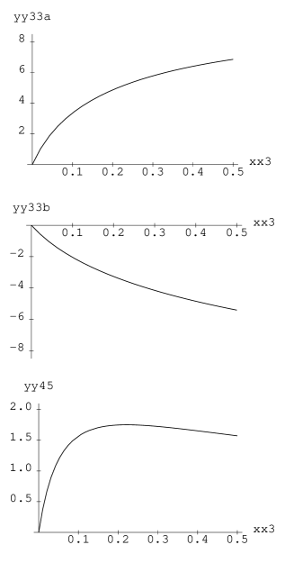
FIG. 8.: ${\cal O}(p^{3})$ HBChPT results for the three redundant spin polarizabilities of Eq.(151), reconstructed from the C-invariance constraints of Eq.(26). Note that the “anomaly-contributions” of appendix D are not included here but plotted separately in Fig.12.

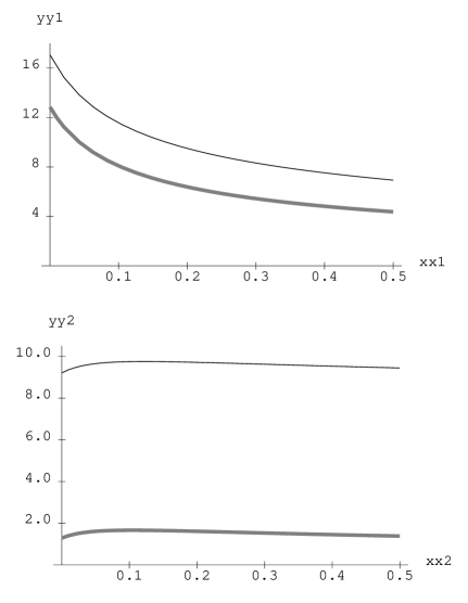
FIG. 9.: Absolute ${\cal O}(\epsilon^{3})$ SSE results for the two spin-independent generalized polarizabilities $\bar{\alpha}_{E}^{(III)}(\bar{q}^{2}),\;\bar{\beta}_{M}^{(III)}(\bar{q}^{2})$ of Eq.(159), compared to the ${\cal O}(p^{3})$ HBChPT results shown in gray shading.

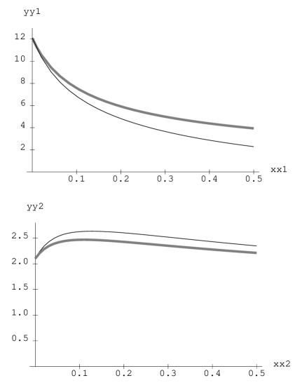
FIG. 10.: Comparison between the ${\cal O}(\epsilon^{3})$ SSE results for $\bar{\alpha}_{E}^{ren.}(\bar{q}^{2}),\;\bar{\beta}_{M}^{ren.}(\bar{q}^{2})$ with ${\cal O}(p^{3})$ HBCHPT (in gray shading). Note that all curves have been normalized to the experimental results of $\bar{\alpha}_{E},\;\bar{\beta}_{M}$ of the proton at the real photon point $\bar{q}\rightarrow 0$.

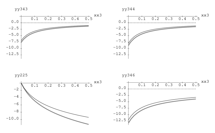
FIG. 11.: ${\cal O}(\epsilon^{3})$ SSE results for the four independent generalized spin polarizabilities of Eq.(191), compared to the ${\cal O}(p^{3})$ HBChPT results of Eq.(148) in gray shading. Note that the “anomaly-contributions” of appendix D are not included but plotted separately in Fig.12.

FIG. 12.: ${\cal O}(p^{3})$ HBChPT/${\cal O}(\epsilon^{3})$ SSE $\pi^{0}$-pole contributions to the generalized spin polarizabilities.

REFERENCES

- [1] See, e.g., A.I. L’vov, Int. J. Mod. Phys. A8, 5267 (1993); B.R. Holstein, Comm. Nucl. Part. Phys. 20, 301 (1992).
- [2] F.J. Federspiel et al., Phys. Rev. Lett. 67, 1511 (1991); A.L. Hallin et al., Phys. Rev. C48, 1497 (1993); A. Zieger et al., Phys. Lett. B278, 34 (1992); B.E. MacGibbon et al., Phys. Rev. C52, 2097 (1995).
- [3] J. Schmiedmayer et al., Phys. Rev. Lett. 66, 1015 (1991).
- [4] L. Koester, Phys. Rev. C51, 3363 (1995).
- [5] S. Beane, M. Malheiro, D.R. Phillips, and U. van Kolck, nucl-th/9905023; to appear in Nucl. Phys. A.
- [6] D. Babusci, G. Giordano, and G. Matone, Phys. Rev. C57, 291 (1998).
- [7] S. Ragusa, Phys. Rev. D47, 3757 (1993); ibid. D49, 3157 (1994).
- [8] See, e.g. D. Babusci, G. Giordano, A. L’vov, and A. Nathan, Phys. Rev. C58, 1013 (1998).
- [9] A.M. Sandorfi et al., Phys. Rev. D50, R6681 (1994).
- [10] J. Tonnison et al., Phys. Rev. Lett. 80, 4382 (1998).
- [11] D. Drechsel, G. Krein, and O. Hanstein, Phys. Lett. B420, 248 (1998); D. Drechsel, M. Gorchtein, B. Pasquini, and M. Vanderhaeghen, hep-ph/9904290.
- [12] J. Roche et al., “The first dedicated Virtual Compton Scattering experiment at MAMI”; forthcoming.
- [13] T.R. Hemmert, B.R. Holstein, G. Knöchlein and S. Scherer, Phys. Rev. D55, 2630 (1997).
- [14] T.R. Hemmert, B.R. Holstein, G. Knöchlein and S. Scherer, Phys. Rev. Lett. 79, 22 (1997).
- [15] T.R. Hemmert, B.R. Holstein, and J. Kambor, Phys. Lett. B395, 89 (1997).
- [16] T.R. Hemmert, B.R. Holstein and J. Kambor, Phys. Rev. D55, 5598 (1997)
- [17] T.R. Hemmert, B.R. Holstein, J. Kambor and G. Knöchlein, Phys. Rev. D57 5746, (1998).
- [18] See, e.g., Proc. Workshop on Virtual Compton Scattering VCS96, Clermont-Ferrand, 1996, Ed. V. Breton; P.A.M. Guichon and M. Vanderhaeghen, Prog. in Part. and Nucl. Phys. 41, 125 (1998).
- [19] J. Edelmann, N. Kaiser, G. Piller and W. Weise, Nucl. Phys. A641, 119 (1998); D. Drechsel, S.S. Kamalov, G. Krein, B. Pasquini, and L. Tiator, nucl-th/9907056, to be published in Nucl. Phys. A; X. Ji and J. Osborne, hep-ph/9905410.
- [20] R.A. Berg and C.N. Lindner, Nucl. Phys. 26, 259 (1961); H. Arenhövel and D. Drechsel, Nucl. Phys. A233, 153 (1974).
- [21] P.A.M. Guichon, G.Q. Liu, and A.W. Thomas, Nucl. Phys. A591, 606 (1995) and Aust. J. Phys. 49, 905 (1996).
- [22] D. Drechsel, G. Knöchlein, A. Metz, and S. Scherer, Phys. Rev. C55, 424 (1997).
- [23] D. Drechsel, G. Knöchlein, A. Yu. Korchin, A. Metz, and S. Scherer, Phys. Rev. C57, 941 (1998).
- [24] A. Metz and D. Drechsel, Z. Phys. A356, 351 (1996) and A359, 165 (1997).
- [25] M. Vanderhaeghen, Phys. Lett. B368, 13 (1996).
- [26] M. Kim and D.-P. Min, hep-ph/9704381.
- [27] V. Bernard, N. Kaiser, and U.-G. Meißner, Int. J. Mod. Phys. E4, 193 (1995).
- [28] V. Bernard, H.W. Fearing, T.R. Hemmert and U.-G. Meißner, Nucl. Phys. A635, 121 (1998); (E) A642, 536 (1998).
- [29] J. Gasser and H. Leutwyler, Ann. Phys. (NY) 158, 142 (1984); Nucl. Phys. B250, 465 (1985).
- [30] J. Wess and B. Zumino, Phys. Lett. B37, 95 (1971); E. Witten Nucl. Phys. B223, 422 (1983).
- [31] V. Bernard, J. Kambor, N. Kaiser, and U.-G. Meißner, Nucl. Phys. B388, 315 (1992).
- [32] T.R. Hemmert, B.R. Holstein, and J. Kambor, J. Phys. G24, 1831 (1998).
- [33] T.R. Hemmert, University of Massachusetts Ph.D. Thesis, Amherst 1997, UMI-98-09346-mc (microfiche).
- [34] A. Manohar and H. Georgi, Nucl. Phys. B234, 189 (1984); J.F. Donoghue, E. Golowich, and B.R. Holstein, Phys. Rev. D30, 587 (1984).
- [35] F.E. Low, Phys. Rev. 96, 1428 (1954); M. Gell-Mann and M.L. Goldberger, Phys. Rev. 96, 1433 (1954).
- [36] S. Scherer, A.Yu. Korchin, and J.H. Koch, Phys. Rev. C54, 904 (1996).
- [37] G. Knöchlein, Universität Mainz Ph.D. Thesis, Shaker Verlag (Aachen) 1997.
- [38] C. Unkmeir, S. Scherer, A.I. L’vov, and D. Drechsel, hep-ph/9904442.
- [39] See, e.g., N.C. Mukhopadhyay, A.M. Nathan and L. Zhang, Phys. Rev. D47, R7 (1993).
- [40] V. Bernard, N. Kaiser, A. Schmidt, and U.-G. Meißner, Phys. Lett. B319, 269 (1993); Z. Phys. A348, 317 (1994).
- [41] G. Gellas, T.R. Hemmert, C. Ktorides and U.-G. Meißner, forthcoming.