Small size boundary effects on two-pion interferometry

Abstract

Bose-Einstein correlations of two identically charged pions are derived when these particles, the most abundantly produced in relativistic heavy ion collisions, are confined in finite volumes. Boundary effects on single-pion spectrum are also studied. Numerical results emphasize that conventional formulation usually adopted to describe two-pion interferometry should not be used when the source size is small, since this is the most sensitive case to boundary effects. Specific examples are considered for better illustration.

I Introduction

It is generally expected that high energy heavy-ion collisions may provide the tools to probe the existence of a new phase of matter of strongly interaction particles, the quark-gluon plasma (QGP), at high temperature and high baryon density[1]. The hope of discovering the QGP in high energy heavy-ion collisions is to some extent connected to the possibility of measuring the geometrical sizes of the emission region of secondary particles. An important tool for accomplishing such size measurements is the so-called Hanbury-Brown-Twiss (HBT) interferometry[2]. This method was originally proposed in the 50’s for measuring stellar radii but, shortly afterwards, it was discovered[3] that a similar procedure could also be applied to high energy collisions for determining the dimensions of pion emitting sources. This method has extensively been developed, improved, and better understood since the pioneering times[4].

Differently from the stellar case, however, where the dimensions are indeed immense, in the subatomic level the effects associated to the small sizes of the particle emitters and their boundaries may have an important role. Indeed, already in the well-known paper by Gyulassy, Kauffmann, and Wilson[5], and more recently, in Ref.[6, 7, 8, 9, 10, 11], effects of source finiteness on particle spectra and correlation functions were considered, although the conclusions of some of them were somewhat contradictory. For example, the low transverse momentum region of Ref.[8, 11] is shown to be enhanced with respect to the Bose-Einstein distribution. However, this enhancement was not observed in other references quoted above. As we shall see later, in agreement with results of Ref.[7, 9, 10], a depletion in the low momentum region is observed instead. This apparent discrepancy may be explained by both the form chosen for the density matrix in Ref.[8, 11], and by the full field theoretical approach adopted there. However, the inherent difficulties of that approach are enormous, and the simpler treatment discussed in the present paper already sheds light to the relevant points of the problem.

The approach suggested in Ref.[7, 9] seemed appealing for the following reasons. First, it considers that in an ultra-relativistic nucleus-nucleus collisions pions are the most abundant produced particles, being emitted at freeze-out temperatures around 0.1-0.2 GeV. Following Ref.[9, 10], it is argued that right after these collisions, since the average pion separation is smaller than their interaction range, the pions in such a stage of the system evolution are still strongly interacting with each other. The effects of interaction among pions could then be modeled by considering that they are moving in an attractive mean field potential, which extends over the whole pion system. This implies, for instance, that in the two-pion case, they would not suffer any other effects besides the mean field attraction and the identical particle symmetrization. Consequently, rather than being in a gas, the pion system should be considered in a quasi-bound liquid phase, with the surface tension[12] acting as a reflecting boundary. Although details on this reflection depend on the pion wavelength, the pion wave function could be considered as vanishing outside this boundary. The pions become free when their average separation is larger than their interaction range. Due to the short range of the strong interaction, however, we would expect this liquid-gas transition to happen very rapidly, in such a way that the momentum distribution of pions could be essentially governed by their momentum distribution just before they freeze out. Under these circumstances, we would also expect that the observed pion momentum distribution would be modified by the presence of this boundary. And this is, in fact, what is analyzed in this work, as well as in Ref.[7, 8, 9, 10, 11].

On the other hand, since pion interferometry is sensitive to the geometrical size of the emission region as well as to the underlying dynamics, we would expect that the boundary would also affect the correlation function, but a priori we would not know how. Would it affect single- and double inclusive distributions similarly? How would be intercept of the two-particle correlation function behave? How would the general shape of this function be affected? For an insight into these questions, we here investigate the effects exerted by the boundary on the two-particle correlation function. We could naively expect that the importance of quantum statistics would progressively increase as the dimension of the emission region decreases. The results turned to exactly fulfill these expectations. Consequently, semi-classical approaches would have their applicability limited by the size of the emission region in focus. In other words, small emission volumes would stress the need for quantum statistics and, as a consequence, classical density matrices would lead to inconsistent results. This problem is clearly illustrated later in the present work.

The plan of this paper is the following: in section II, we derive the single-inclusive distribution, as well as the two-pion correlation function, considering a density matrix suited for describing $\pi^{\pm}\pi^{\pm}$ Bose-Einstein effects. In section III, the boundary effects on the two-pion correlation and single particle spectrum distribution are illustrated by means of two specific examples. Section IV is devoted to illustrate the results which would be expected when previous methods for deriving two-pion interferometry formula are employed and the finite volume effects are studied. Finally, conclusions are discussed in section V.

II Spectrum and Two-pion correlation function

In this section, we derive a generic formulation for the single- as well as for the two-particle inclusive distributions, which would be suited for describing $\pi^{+}\pi^{+}$ or $\pi^{-}\pi^{-}$ bounded in a finite volume.

We assume the pion creation operator in coordinate space can be expressed as

$$\hat{\psi}^{\dagger}({\bf x})=\sum_{\lambda}\hat{a}^{\dagger}_{\lambda}\psi^{*}_{\lambda}({\bf x}),$$ (1)

where $a^{\dagger}_{\lambda}$ is the creation operator for creating a pion in a quantum state characterized by a quantum number $\lambda$. Then, $\psi_{\lambda}({\bf x})$ is one of eigenfunctions belonging to a localized complete set, which satisfies the orthonormality condition

$$\int d{\bf x}\psi^{*}_{\lambda}({\bf x})\psi_{\lambda^{\prime}}({\bf x})=\delta_{\lambda,\lambda^{\prime}},$$ (2)

and completeness relation

$$\sum_{\lambda}\psi^{*}_{\lambda}({\bf x})\psi_{\lambda}({\bf y})=\delta({\bf x}-{\bf y}).$$ (3)

Similarly, the pion annihilation operator in coordinate space can be written as

$$\hat{\psi}({\bf x})=\sum_{\lambda}\hat{a}_{\lambda}\psi_{\lambda}({\bf x}).$$ (4)

In momentum space, the corresponding pion creation operator, $\hat{\psi}^{\dagger}({\bf p})$, and annihilation operator, $\hat{\psi}({\bf p})$, can be expressed as

$$\hat{\psi}^{\dagger}({\bf p})=\sum_{\lambda}\hat{a}^{\dagger}_{\lambda}\tilde{\psi}^{*}_{\lambda}({\bf p})$$ (5)

and

$$\hat{\psi}({\bf p})=\sum_{\lambda}\hat{a}_{\lambda}\tilde{\psi}_{\lambda}({\bf p}),$$ (6)

where

$$\tilde{\psi}_{\lambda}({\bf p})=\frac{1}{(2\pi)^{3/2}}\int\psi_{\lambda}({\bf x})e^{i{\bf p}\cdot{\bf x}}d{\bf x}.$$ (7)

We write the density matrix operator for our bosonic system as

$$\hat{\rho}=\exp\left[-\frac{1}{T}(\hat{H}-\mu\hat{N})\right]\;\;,$$ (8)

where

$$\hat{H}=\sum_{\lambda}E_{\lambda}a^{\dagger}_{\lambda}a_{\lambda},\;\;\hat{N}=\sum_{\lambda}a^{\dagger}_{\lambda}a_{\lambda}\;\;,$$ (9)

are the Hamiltonian and number operators, respectively; T is the temperature.

The corresponding normalization is explicitly included in the definition of the expectation value of observables as, for instance, for an operator $\hat{A}$

$$\langle\hat{A}\rangle=\frac{tr\{\hat{\rho}\hat{A}\}}{tr\{\hat{\rho}\}}\;\;.$$ (10)

Then, the single-pion distribution can be written as

$$P_{1}({\bf p}) = \langle\hat{\psi}^{\dagger}({\bf p})\hat{\psi}({\bf p})\rangle$$ (11)

$$= \sum_{\lambda}\sum_{\lambda^{\prime}}\tilde{\psi}_{\lambda}^{*}{(\bf p)}\tilde{\psi}_{\lambda^{\prime}}^{*}{(\bf p)}\langle\hat{a}^{\dagger}_{\lambda}\hat{a}_{\lambda^{\prime}}\rangle\;\;.$$ (12)

The expectation value $\langle\hat{a}^{\dagger}_{\lambda}\hat{a}_{\lambda^{\prime}}\rangle$ is related to the occupation probability of the single-particle state $\lambda$, $N_{\lambda}$, by

$$\langle\hat{a}^{\dagger}_{\lambda}\hat{a}_{\lambda^{\prime}}\rangle=\delta_{\lambda,\lambda^{\prime}}N_{\lambda}\;\;;$$ (13)

for a bosonic system in equilibrium at a temperature $T$ and chemical potential $\mu$, it is represented by the Bose-Einstein distribution

$$N_{\lambda}=\frac{1}{\exp{\left[\frac{1}{T}(E_{\lambda}-\mu)\right]}-1}\;\;.$$ (14)

By inserting Eq. (13) and (14) into (12), we obtain the single-particle spectrum for one pion species as

$$P_{1}({\bf p})=\sum_{\lambda}N_{\lambda}\tilde{\psi}^{*}_{\lambda}({\bf p})\tilde{\psi}_{\lambda}({\bf p})\;.$$ (15)

The above formula coincides with the one employed in Ref.[9] for expressing the single-pion distribution.

Similarly, the two-pion distribution function can be written as

$$P_{2}({\bf p_{1},p_{2}}) = \langle\hat{\psi}^{\dagger}({\bf p_{1}})\hat{\psi}^{\dagger}({\bf p_{2}})\hat{\psi}({\bf p_{1}})\hat{\psi}({\bf p_{2}})\rangle$$ (16)

$$= \sum_{\lambda_{1},\lambda_{2},\lambda_{3},\lambda_{4}}\tilde{\psi}_{\lambda_{1}}^{*}({\bf p_{1}})\tilde{\psi}_{\lambda_{2}}^{*}({\bf p_{2}})\tilde{\psi}_{\lambda_{3}}({\bf p_{1}})\tilde{\phi}_{\lambda_{4}}({\bf p_{2}})$$ (18)

$$\langle\hat{a}^{\dagger}_{\lambda_{1}}\hat{a}^{\dagger}_{\lambda_{2}}\hat{a}_{\lambda_{3}}\hat{a}_{\lambda_{4}}\rangle$$

$$= \sum_{\lambda_{1},\lambda_{2},\lambda_{3},\lambda_{4}}\tilde{\psi}_{\lambda_{1}}^{*}({\bf p_{1}})\tilde{\psi}_{\lambda_{2}}^{*}({\bf p_{2}})\tilde{\psi}_{\lambda_{3}}({\bf p_{1}})\tilde{\phi}_{\lambda_{4}}({\bf p_{2}})$$ (24)

$$\left[\langle\hat{a}^{\dagger}_{\lambda_{1}}\hat{a}_{\lambda_{3}}\rangle\langle\hat{a}^{\dagger}_{\lambda_{2}}\hat{a}_{\lambda_{4}}\rangle_{\lambda_{1}\neq\lambda_{2}}\right.$$

$$+\langle\hat{a}^{\dagger}_{\lambda_{1}}\hat{a}_{\lambda_{4}}\rangle\langle\hat{a}^{\dagger}_{\lambda_{2}}\hat{a}_{\lambda_{3}}\rangle_{\lambda_{1}\neq\lambda_{2}}$$

$$\left.+\langle\hat{a}^{\dagger}_{\lambda_{1}}\hat{a}^{\dagger}_{\lambda_{2}}\hat{a}_{\lambda_{3}}\hat{a}_{\lambda_{4}}\rangle_{\lambda_{1}=\lambda_{2}=\lambda_{3}=\lambda_{4}}\right]$$

$$=P_{1}({\bf p_{1}})P_{1}({\bf p_{2}})+\sum_{\lambda_{1}}\sum_{\lambda_{2}}$$

$$N_{\lambda_{1}}N_{\lambda_{2}}\tilde{\psi}^{*}_{\lambda_{1}}({\bf p_{1}})\tilde{\psi}_{\lambda_{1}}({\bf p_{2}})\tilde{\psi}^{*}_{\lambda_{2}}({\bf p_{1}})\tilde{\psi}_{\lambda_{2}}({\bf p_{2}})$$

$$= P_{1}({\bf p_{1}})P_{1}({\bf p_{2}})+|\sum_{\lambda}N_{\lambda}\tilde{\psi}_{\lambda}^{*}({\bf p_{1}})\tilde{\psi}_{\lambda}({\bf p_{2}})|^{2}.$$ (25)

Since we are considering the case of two indistinguishable, identically charged pions, then

$$\langle\hat{a}_{\lambda}^{\dagger}\hat{a}_{\lambda}^{\dagger}\hat{a}_{\lambda}\hat{a}_{\lambda}\rangle=2\langle\hat{a}^{\dagger}_{\lambda}\hat{a}_{\lambda}\rangle^{2}.$$ (27)

From the particular form proposed for the density matrix in Eq. (8), we can see that $\langle\hat{a}^{\dagger}_{\lambda}\hat{a}^{\dagger}_{\lambda}\rangle=\langle\hat{a}_{\lambda}\hat{a}_{\lambda}\rangle=0$, showing that it would not be suited for describing $\pi^{0}\pi^{0}$ and $\pi^{+}\pi^{-}$ cases. For this purpose, the formalism proposed in Ref.[6, 8, 11] may be more adequate.

The two-particle correlation can be written as

$$C_{2}({\bf p_{1},p_{2}}) = \frac{P_{2}({\bf p_{1},p_{2}})}{P_{1}({\bf p_{1}})P_{1}({\bf p_{2}})}$$ (28)

$$= 1+\frac{|\sum_{\lambda}N_{\lambda}\tilde{\psi}_{\lambda}^{*}({\bf p_{1}})\tilde{\psi}_{\lambda}({\bf p_{2}})|^{2}}{\sum_{\lambda}N_{\lambda}|\tilde{\psi}_{\lambda}({\bf p_{1}})|^{2}\sum_{\lambda}N_{\lambda}|\tilde{\psi}_{\lambda}({\bf p_{2}})|^{2}}\;\;.$$ (29)

We can see immediately from the above formula that if ${\bf q}={\bf p_{1}}-{\bf p_{2}}=0$ we have $C_{2}({\bf p,p})=2$. We also notice that the result for the correlation function in Eq. (LABEL:pi2) reflects the symmetrization over different states (and thus, the uncertainty in the determination of the pion state).

Within this formulation we can also define the corresponding Wigner function, $g({\bf x},{\bf K})$, as

$$g({\bf x},{\bf K}) = \frac{1}{(2\pi)^{3}}\sum_{\lambda}N_{\lambda}\int\psi_{\lambda}^{*}\left({\bf x+\frac{y}{2}}\right)\psi_{\lambda}\left({\bf x-\frac{y}{2}}\right)$$ (32)

$$\exp(-i{\bf K}\cdot{\bf y})d{\bf y},$$

Consequently, we can write

$$\langle\hat{\psi}^{\dagger}({\bf p_{1}})\hat{\psi}({\bf p_{2}})\rangle = \sum_{\lambda}N_{\lambda}\tilde{\psi}^{*}_{\lambda}({\bf p_{1}})\tilde{\psi}_{\lambda}({\bf p_{2}})$$ (33)

$$= \int e^{-i({\bf p_{1}-p_{2}})\cdot{\bf x}}\;g({\bf x},{\bf k})d{\bf x}.$$ (34)

By means of this Wigner function, the two-pion interferometry formula can be re-written as[13, 14, 15]

$$C_{2}({\bf p_{1},p_{2}}) = 1+$$ (36)

$$\frac{\int e^{i{\bf q}\cdot({\bf x-y})}g({\bf x},{\bf K})g({\bf y},{\bf K})d{\bf x}d{\bf y}}{\int g({\bf x},{\bf p_{1}})g({\bf y},{\bf p_{2}})d{\bf x}d{\bf y}}.$$

In the above equation, ${\bf K=(p_{1}+p_{2})}/2$ is the two-pion average momentum, and ${\bf q=p_{1}-p_{2}}$ is their relative momentum. Here $g({\bf x,K})$ can be interpreted as the probability of finding a pion at point x with momentum K.

III Two-pion correlation from a finite volume

A Example 1

In order to investigate the effect of the boundary on the single- and on the two-pion distribution functions, we assume that pions produced in high energy heavy-ion collisions are bounded in a sphere, just before freezing-out. In other words, their distribution functions are essentially the the ones they had while confined. The pion wave function should be determined by the solution of the Klein-Gordon equation

$$\left[\Delta+k^{2}\right]\psi({\bf r})=0\;\;,$$ (37)

where $k^{2}=E^{2}-m^{2}$ is the momentum of the pion. On writing the above equation, we have assumed that the potential felt by the pion inside the sphere is zero, while outside it is infinite. The boundary condition to be respected by the solution is

$$\psi({\bf r})|_{r=R}=0\;\;,$$ (38)

where $R$ is the radius of the sphere at freeze-out time.

The normalized wave function corresponding to the solution of the above equation can easily be written as

$$\psi_{klm}({\bf r}) = \frac{1}{RJ_{l+\frac{3}{2}}(kR)}\sqrt{\frac{2}{r}}Y_{lm}(\theta,\phi)J_{l+\frac{1}{2}}(kr)~{}~{}~{}~{}(r<R),$$ (39)

$$= 0~{}~{}~{}~{}~{}~{}~{}~{}~{}~{}~{}~{}~{}~{}~{}~{}~{}~{}~{}~{}~{}~{}~{}~{}~{}~{}~{}~{}~{}~{}~{}~{}~{}~{}~{}~{}~{}~{}~{}~{}~{}~{}~{}~{}~{}~{}~{}(r\geq R).$$ (40)

The momentum of the bounded particle, $k$, can be determined as the solution of the equation

$$J_{l+\frac{1}{2}}(kR)=0\;\;.$$ (42)

Inserting Eq. (23) into Eq. (7), we can determine the Fourier transform of the confined solution of a pion inside the sphere, as a function of the momentum p, as

$$\tilde{\psi}_{klm}({\bf p})=\sqrt{\frac{2}{p}}i^{l}Y_{lm}(\hat{p})\frac{1}{RJ_{l+\frac{3}{2}}(kR)}\left(\frac{R}{p^{2}-k^{2}}\right)$$ (45)

$$\left[pJ_{l+\frac{3}{2}}(pR)J_{l+\frac{1}{2}}(kR)-kJ_{l+\frac{1}{2}}(pR)J_{l+\frac{3}{2}}(kR)\right]$$

$$~{}~{}~{}~{}~{}~{}~{}~{}~{}~{}~{}~{}~{}~{}~{}~{}~{}~{}~{}~{}~{}~{}~{}~{}~{}~{}~{}~{}~{}~{}~{}~{}~{}~{}~{}~{}~{}~{}~{}~{}~{}(p\neq k),$$

$$= \sqrt{\frac{1}{2p}}\;i^{l}\;Y_{lm}(\hat{p})\;RJ_{l+\frac{3}{2}}(kR)\;~{}\;~{}~{}~{}~{}(p=k).$$ (46)

On deriving the above equation, we have made use the following integral equations

$$\int_{0}^{R}rdrJ_{l+1/2}(pr)J_{l+\frac{1}{2}}(kr)=\frac{R}{p^{2}-k^{2}}$$ (47)

$$\left[\frac{}{}pJ_{l+\frac{3}{2}}(pR)J_{l+\frac{1}{2}}(kR)-kJ_{l+\frac{1}{2}}(pR)J_{l+\frac{3}{2}}(kR)\right],$$ (48)

and

$$\int_{0}^{R}rdrJ_{l+\frac{1}{2}}(kr)J_{l+\frac{1}{2}}(kr) = \frac{R^{2}}{2}J^{2}_{l+\frac{3}{2}}(kR)\;\;.$$ (49)

Besides, by imposing that the solution should vanish at the boundary, expressed by Eq. (42), it can be shown that

$$\lim_{p\rightarrow k}\frac{pJ_{l+3/2}(pR)J_{l+1/2}(kR)-kJ_{l+\frac{1}{2}}(pR)J_{l+\frac{3}{2}}(kR)}{p^{2}-k^{2}}$$ (50)

$$=\frac{RJ^{2}_{l+\frac{3}{2}}(kR)}{2}\;\;,$$ (51)

i.e., $\tilde{\psi}_{klm}({\bf p})$ is a continuous function of $p$ at $p=k$.

Using the condition expressed by Eq. (42), Eq. (46) can be further simplified as

$$\tilde{\psi}_{klm}({\bf p})=\sqrt{\frac{2}{p}}i^{l}Y_{lm}(\hat{p})\left[\frac{-k}{p^{2}-k^{2}}\right]J_{l+\frac{1}{2}}(pR)\;\;.$$ (52)

In terms of Eq. (49), the single-inclusive distribution function is given by

$$P_{1}({\bf p}) = \sum_{klm}N_{klm}\tilde{\psi}_{klm}^{*}({\bf p})\tilde{\psi}_{klm}({\bf p})$$ (53)

$$= \sum_{klm}\frac{1}{\exp{(\frac{E_{kl}-\mu}{T})}-1}\sqrt{\frac{2}{p}}(-i)^{l}Y^{*}_{lm}(\hat{p})\sqrt{\frac{2}{p}}i^{l}$$ (55)

$$Y_{lm}(\hat{p})\left[\frac{-k\cdot J_{l+\frac{1}{2}}(pR)}{p^{2}-k^{2}}\right]\left[\frac{-k\cdot J_{l+\frac{1}{2}}(pR)}{p^{2}-k^{2}}\right]$$

$$= \sum_{k,l}\frac{1}{\exp{(\frac{E_{kl}-\mu}{T})}-1}\left(\frac{2l+1}{2\pi p}\right)\left(\frac{kJ_{l+\frac{1}{2}}(pR)}{p^{2}-k^{2}}\right)^{2},$$ (56)

where we have used that

$$\sum_{m=-l}^{m=l}Y_{lm}^{*}(\hat{p}_{1})Y_{lm}(\hat{p}_{2})=\left(\frac{2l+1}{4\pi}\right)P_{l}(\hat{p}_{1}\cdot\hat{p}_{2}).$$ (58)

Up to this point we have considered the pions confined in a sphere, which required the wave function to have a sharp change at $r=R$. However, as discussed in Ref.[16], it could be more appropriate to consider a smoother boundary, by softening the potential felt by the pion at $r=R$. Unfortunately, this procedure would turn the problem into a very complex one [16], and beyond the scope of this paper. Nevertheless, as a diffuse boundary would cause a gradual decrease to zero of the pion wave function, it could be simulated by taking the limit $R\rightarrow\infty$ [16] in Eq. (48), i.e.,

$$\int_{0}^{\infty}J_{l+\frac{1}{2}}(pr)J_{l+\frac{1}{2}}(kr)rdr=\frac{1}{k}\delta(p-k)$$ (59)

and

$$J_{l+\frac{3}{2}}(kR)\rightarrow\sqrt{\frac{2}{\pi kR}}$$ (60)

$$\tilde{\psi}_{klm}=i^{l}Y_{lm}(\hat{p})\sqrt{\frac{\pi}{pkR}}\delta(p-k).$$ (61)

Then, by imposing the completeness relation, Eq. (3), we can show that

$$\sum_{\lambda}\tilde{\psi}_{\lambda}^{*}({\bf p})\tilde{\psi}_{\lambda}({\bf p})=\frac{V}{(2\pi)^{3}}$$ (62)

With the $\delta$ function in Eq. (59) and Eq. (61), the single particle spectrum, in the limit $R\rightarrow\infty$, is then written as

$$P_{1}({\bf p})=\frac{1}{\exp{(\frac{E_{p}-\mu}{T})}-1}\left[\frac{V}{(2\pi)^{3}}\right]\;\;,$$ (63)

where $V=\frac{4\pi}{3}R^{3}$ is the volume of the sphere. We see from Eq. (63) that the ordinary Bose Einstein distribution is recovered in the limit of a very large volume.

For $p=0$ and $V=\frac{4\pi}{3}R^{3}$, Eq. (LABEL:P1sph1) becomes

$$P_{1}({\bf p})|_{p=0}=V\sum_{n=1}^{\infty}\frac{1}{\exp{(\frac{E_{n}-\mu}{T})}-1}\left(\frac{3}{4\pi^{5}n^{2}}\right)\;\;,$$ (64)

where

$$E_{n}=\sqrt{\left(\frac{n\pi}{R}\right)^{2}+m_{\pi}^{2}}\;\;.$$ (65)

In the limit $R\rightarrow\infty$, we have

$$P_{1}({\bf p})=\left[\frac{V}{(2\pi)^{3}}\right]\frac{1}{\exp(\frac{m_{\pi-\mu}}{T})-1}\;\;,$$ (66)

which is consistent with Eq. (63).

From Eq. (64), we see that the intercept of the spectrum depends on the value of the radius: as $R$ increases, $E_{n}$ becomes smaller, and the maximum value of this distribution, corresponding to $|{\bf p}|=0$, becomes higher. In all numerical estimates considered in the present work we have fixed $\mu=0$. In Figure 1, the normalized single-particle distribution is plotted as a function of $|{\bf p}|$. We have chosen a discrete normalization, obtained by imposing ${\cal N}=\sum_{i=1}^{N}P_{1}(p_{i})$, where N refers to the total number of bins in which the distribution is subdivided.

We clearly see from Figure 1 that, due to the boundary effects, the maximum value of $|{\bf p}|$ in the spectrum decreases for decreasing volumes, being always smaller than the case corresponding to the $R\rightarrow\infty$ limit. The explanation for this behavior can be understood in terms of the uncertainty principle, i.e., as the volume of the system decreases, the uncertainty in the pion coordinate decreases accordingly, causing a large fluctuation in the pion momentum distribution. We should notice that this result coincides with the one obtained in Ref.[7, 9], and is opposite to the results from Ref.[8, 11].

Regarding the spectrum, we could also inquire how would the freeze-out temperature affect it and how would the finite size effect compare with the $R\rightarrow\infty$ limit for different temperatures. This is illustrated in Figure 2. The curves there should be compared in groups of two: solid ($T=0.14$ GeV) and dotted ($T=0.11$ GeV). For emphasizing the differences and similarities as $|{\bf p}|$ increases, we plot the difference between the two curves in each group, $\Delta P_{1}({\bf p})=P_{1}({\bf p})|_{R=3fm}-P_{1}({\bf p})|_{R=\infty}$, in Figure 3. We see that the lower the temperature, the bigger is the difference between the curves of each group, in the small momentum region. Decreasing the temperature has a similar effect on the spectrum as decreasing the radius: in both cases the fluctuations in the small region of the pion spectrum increases and the corresponding maximum is reduced. In other words, the boundary effects are more significant when we deal with systems whose dimensions and temperatures are small.

We should observe that, except in Fig. 2 and 3 where the temperature dependence is studied, we have fixed $T=0.12$ GeV. The reason for this relies on Shuryak’s arguments[12], according to which for temperatures in the range $0.1\leq T\leq 0.2$ GeV, the excited pionic matter would be better described as in a liquid phase inside a surface created by their mutual interaction. He added that, for $T\geq 0.15$ GeV, the influence of resonances become important but they are not included in the present study. Therefore we chose $T=0.12$ GeV, which is also of the order of the recent experimental freeze-out temperature estimated from both interferometry and spectra.

Similarly, we can write for the expectation value of the product of two pion creation operators in momentum space

$$\langle\hat{\psi}^{\dagger}({\bf p_{1}})\hat{\psi}({\bf p_{2}})\rangle=\sum_{klm}\frac{\tilde{\psi}^{*}_{klm}({\bf p_{1}})\tilde{\psi}_{klm}({\bf p_{2}})}{\exp{\left(\frac{E_{kl}-\mu}{T}\right)}-1}$$ (67)

$$= \sum_{klm}\frac{1}{\exp{\left(\frac{E_{kl}-\mu}{T}\right)}-1}\times$$ (70)

$$\sqrt{\frac{2}{p_{1}}}(-i)^{l}Y_{lm}^{*}(\hat{p}_{1})\left[\frac{-k}{p_{1}^{2}-k^{2}}\right]J_{l+\frac{1}{2}}(p_{1}R)$$

$$\sqrt{\frac{2}{p_{2}}}(i)^{l}Y_{lm}^{*}(\hat{p}_{2})\left[\frac{-k}{p_{2}^{2}-k^{2}}\right]J_{l+\frac{1}{2}}(p_{2}R)$$

$$= \sum_{kl}\frac{1}{\exp{\left(\frac{E_{kl}-\mu}{T}\right)}-1}\sqrt{\frac{4}{p_{1}p_{2}}}$$ (73)

$$\frac{k^{2}}{(p_{1}^{2}-k^{2})(p_{2}^{2}-k^{2})}J_{l+\frac{1}{2}}(p_{1}R)$$

$$J_{l+\frac{1}{2}}(p_{2}R)\left(\frac{2l+1}{4\pi}\right)P_{l}(\hat{p}_{1}\cdot\hat{p}_{2})\;\;.$$

The two-pion interferometry correlation function can then be estimated by inserting the above expression into Eq. (LABEL:pi2). In general, this function will depend on the angle between ${\bf p_{1}}$ and ${\bf p_{2}}$. For the sake of simplicity, we will consider ${\bf p_{1}}$ parallel to ${\bf p_{2}}$, implying that $P_{l}(\hat{{\bf p}}_{1}\cdot\hat{{\bf p}}_{2}=\pm 1)=(\pm 1)^{l}$. The results for two-pion interferometry corresponding to different values of the pair average momentum ${\bf K=(p_{1}+p_{2})}/2$ but fixed temperature are shown in Figure 4. We can see that, as the pair average momentum increases, the apparent source radius becomes bigger, which is an interesting behavior, if we compare to results corresponding to expanding systems. In this last case, the probed part of the system decreases with increasing average momentum. Naturally, our present approach does not consider the effects of expansion and the enlargement of the system’s apparent dimensions with increasing K, seen in Figure 4, has its origin in the strong sensitivity to the dynamical matrix. This can be better understood by observing the presence of the weight factor $N_{\lambda}$ in Eq.(LABEL:pi2), with $N_{\lambda}$ expressed in Eq.(14). The increase of the average momentum reflects the increase in the individual momenta ${\bf p_{1}}$ and ${\bf p_{2}}$, which comes from larger values of the sum coefficient, $k$, in Eq.(LABEL:pi2). This has two opposite effects: the factors $1/(p_{i}^{2}-k^{2})$ give larger contribution for $k\sim p_{i}$. However, bigger values of $k$ would also make the exponential factor (with $\mu=0$) drop faster. Being so, by increasing K we are effectively including a larger number of $k$ coefficients that contributes to the sum in Eq.(LABEL:pi2), with decreasing weight $\sim\exp{(-E_{kl}/T)}$. The interference of these extra terms corresponding to larger $k$ with the terms already considered in the sum would make the correlation function drop faster, consequently becoming narrower. Alternatively, we could understand these results by noticing that pions with larger momentum come from larger quantum $\lambda$ states which, in turn, correspond to a smaller spread in coordinate space. As the weight factor in Eq. (LABEL:pi2) is of Bose-Einstein form, larger quantum states will give a smaller contribution to the source distribution, causing the effective source radius to appear larger. In order to confirm that the weight factor in Eq.(LABEL:pi2) is the responsible for the behavior observed in Fig. 4, let us consider the case in which we choose it to be a constant factor, for instance $N_{\lambda}=1$. This situation could be derived from the Bose-Einstein distribution form by considering $T\gg 1$, so that the two-pion interferometry results would become insensitive to the average momentum, due to the very large values of the temperature. The numerical result corresponding to this case is also shown in Fig. 4 (narrower curve). On the other hand, with the help of the completeness relation, Eq.(3), and of Eq.(7), by also assuming that the pions are confined in a sphere, it is straightforward to derive the following $K$ independent two-pion correlation function

$$C_{2}(q)=1+\frac{9}{q^{4}R^{6}}[R\cos(qR)-\frac{\sin(qR)}{q}]^{2}.$$ (74)

For completeness, we also include in Fig. 4 the curve based on Eq.(74), which coincides with our numerically generated curve, cross checking the correctness of our numerical calculation.

Figure 5 shows the two-pion correlation function for increasing values of the spherical radius, i.e., for enlarging volumes. From it, we can clearly see that, as the confining volume increases, the source radius derived from two-pion correlation also increases, as would be expected.

Again, as discussed previously for the spectrum, we could estimate the effect of a diffuse boundary on the two-pion correlation function by considering the limit $R\rightarrow\infty$. By inserting Eq. (61) into Eq. (73), remembering that in this limit we can take $\sum_{k}\rightarrow\int dk$, and using the previous result for the spectrum in this limit, Eq. (63), we finally obtain that

$$\mbox{ $C_{2}({\bf p_{1},p_{2}})$ = }\left\{\begin{array}[]{l}\mbox{1 ~{} ~{} ~{} ~{} ~{} (${\bf p_{1}}$ $\neq$ ${\bf p_{2}}$)}\\ \mbox{2 ~{} ~{} ~{} ~{} ~{} (${\bf p_{1}}$ = ${\bf p_{2}}$)}\\ \end{array}\right.$$ (77)

as would be expected.

To conclude this section we should keep in mind that, if the system size is very small, it would be sensitive to the boundary effects even if we considered a diffuse boundary. On the contrary, if the system size is very large, we would not expect a significant effect in neither the sharp nor the diffuse boundary case[16].

B Example 2

In this subsection, we will study the sensitivity of spectrum and of the two-pion correlation function to the system boundaries, by considering the pion system inside a box of dimensions $L\times L\times L$. We choose first periodic boundary conditions. In this case, the eigenfunction can be written as

$$\psi_{\bf k}({\bf r})=\frac{1}{\sqrt{V}}\exp(-i{\bf k}\cdot{\bf r})\;\;.$$ (78)

Here ${\bf k}$ is the quantum number which satisfies following constraint

$$\mbox{ $k_{i}\cdot L=2\;n_{i}\;\pi$ }\rightarrow\left\{\begin{array}[]{l}\mbox{\boldmath{i=1,2,3}}\\ \mbox{$n_{i}=0,\pm 1,\pm 2,...$ }\\ \end{array}\right.\;\;$$ (81)

The corresponding Fourier transform $\tilde{\psi}_{\bf k}({\bf p})$ can be expressed as

$$\tilde{\psi}_{\bf k}({\bf p}) = \frac{1}{(2\pi)^{3/2}}\frac{8}{\sqrt{V}}\left[\frac{\sin\left[(p_{1}-k_{1})L/2\right]}{p_{1}-k_{1}}\right]$$ (83)

$$\left[\frac{\sin\left[(p_{2}-k_{2})L/2\right]}{p_{2}-k_{2}}\right]\left[\frac{\sin\left[(p_{3}-k_{3})L/2\right]}{p_{3}-k_{3}}\right].$$

The single-particle and two-particle distributions follow from Eq. (15) and (LABEL:p2g). We should notice that, in the limit $L\rightarrow 0$, and using the condition (81), we find the contribution of only one state (${\bf k=0}$) to the two-pion correlation function, resulting in

$$C({\bf p_{1},p_{2}})=2\;\;.\\$$ (84)

On the other hand, if we take the limit of $V\rightarrow\infty$, Eq. (83) becomes

$$\psi_{\bf k}({\bf p})=\frac{1}{\sqrt{V}}(2\pi)^{3/2}\delta({\bf p-k}).$$ (85)

With the above form for $\psi_{\bf k}({\bf p})$ in the limit of very large volumes, we obtain for the correlation function

$$\mbox{ $C_{2}({\bf p_{1},p_{2}})$ = }\left\{\begin{array}[]{l}\mbox{1 ~{} ~{} ~{} ~{} ~{} (${\bf p_{1}}$ $\neq$ ${\bf p_{2}}$)}\\ \mbox{2 ~{} ~{} ~{} ~{} ~{} (${\bf p_{1}}$ = ${\bf p_{2}}$)}\\ \end{array}\right.$$ (88)

If, instead of the periodic boundary conditions, we consider that the pions are confined in the box, i.e., we assume the potential outside it is infinite, then two classes of solutions are possible:

$$\psi^{I}({\bf x})=\sqrt{\frac{8}{V}}\sin(k_{1}\cdot x)\sin(k_{2}\cdot y)\sin(k_{3}\cdot z)\;\;,$$ (89)

with

$$\mbox{ $k_{i}\cdot L=2\;n_{i}\;\pi$ }\rightarrow\left\{\begin{array}[]{l}\mbox{\boldmath{i=1,2,3}}\\ \mbox{$n_{i}=1,2,...$}\\ \end{array}\right.\;\;,$$ (92)

and

$$\psi^{II}({\bf x})=\sqrt{\frac{8}{V}}\cos(k_{1}\cdot x)\cos(k_{2}\cdot y)\cos(k_{3}\cdot z)\;\;,$$ (93)

with

$$\mbox{ $k_{i}\cdot L=(2n_{i}-1)\pi$ }\rightarrow\left\{\begin{array}[]{l}\mbox{\boldmath{i=1,2,3}}\\ \mbox{$n_{i}=1,2,...$}\\ \end{array}\right.\;\;.$$ (96)

It can be shown that, for $V\rightarrow 0$, we have

$$C_{2}^{I,II}({\bf p_{1},p_{2}})=2,$$ (97)

while, for $V\rightarrow\infty$, we obtain

$$\mbox{ $C_{2}^{I,II}({\bf p_{1},p_{2}})$ = }\left\{\begin{array}[]{l}\mbox{1 ~{} ~{} ~{} ~{} ~{} ~{} ~{}(${\bf p_{1}}\neq\pm{\bf p_{2}}$)}\\ \mbox{2 ~{} ~{} ~{} ~{} ~{} ~{} ~{}(${\bf p_{1}}=\pm{\bf p_{2}}$)}\\ \end{array}\right.$$ (100)

The reason for including the ($\pm$) signs in Eq.(100) comes from the parity property of Eq. (89) and (93). From them, it is immediate to see that solution I has negative parity, while solution II has positive parity. The corresponding Fourier transforms then show the same parity property, i.e.,

$$\tilde{\psi}^{I}_{{\bf k}}({\bf p})=-\tilde{\psi}^{I}_{{\bf k}}(-{\bf p})\;\;\;;\;\;\;\tilde{\psi}^{II}_{{\bf k}}(-{\bf p})=\tilde{\psi}^{II}_{{\bf k}}({\bf p})\;\;.$$ (101)

From the above results, we can show that the single particle spectrum and two-pion correlation function correspondingly have the following properties

$$P_{1}^{I,II}({\bf p})=P_{1}^{I,II}(-{\bf p}),$$ (102)

and

$$C_{2}^{I,II}({\bf p_{1},-p_{2}})=C_{2}^{I,II}({\bf p_{1},p_{2}})\;\;.$$ (103)

In particular, we see from Eq. (97), (100), and (103) that, if we choose ${\bf p_{1}=-p_{2}=p}$, we immediately get $C_{2}^{I,II}({\bf p_{1}=-p_{2}=p})=2$ for the confined boundary condition in both volume limits. That is the reason why, as a consequence of the parity property of the wave function, Eq. (100) could be extended to $C_{2}^{I,II}({\bf p_{1}=\pm p_{2}=p})=2$.

For periodical boundary condition, however, we have

$$\tilde{\psi}_{\bf k}({\bf p})=\tilde{\psi}_{-{\bf k}}(-{\bf p}).$$ (104)

Then, for the single particle distribution we will have the following relation

$$P_{1}({\bf p})=P_{1}(-{\bf p}).$$ (105)

Nevertheless, the two-pion correlation function, which can be written as

$$C_{2}({\bf p_{1},-p_{2}})=1+\frac{|\sum_{\bf k}N_{\bf k}\tilde{\psi}_{\bf k}({\bf p_{1}})\tilde{\psi}_{\bf k}(-{\bf p_{2}})|^{2}}{\sum_{\bf k}N_{\bf k}|\tilde{\psi}_{\bf k}({\bf p_{1}})|^{2}\sum_{\bf k}N_{\bf k}|\tilde{\psi}_{\bf k}({\bf p_{2}})|^{2}},$$ (106)

in the case of periodical boundary condition, will show no well-defined property under momentum reflection as the one expressed by Eq. (103).

IV Conventional HBT formulation

We now discuss the case of the conventional formulation, usually adopted in HBT analysis, in terms of classical currents $j(x)$[5] representing the pion sources. For simplicity, we consider the momentum as the only quantum number involved in the problem, i.e., we denote $\{\lambda\}$ as $\{{\bf p}\}$. Besides, we also assume that the pion state could be characterized by the measured momentum. For instance, $\psi({\bf p_{1}})$ represents a pion in a quantum state denoted by ${\bf p_{1}}$. Then the single-particle and the two particle distributions can be written as

$$P_{1}({\bf p})=N({\bf p})\psi^{*}({\bf p})\psi({\bf p}),$$ (107)

and

$$P_{2}({\bf p_{1},p_{2}})=N({\bf p_{1}})N({\bf p_{2}})\psi^{*}({\bf p_{1}})\psi^{*}({\bf p_{2}})\psi({\bf p_{1}})\psi({\bf p_{2}}).$$ (108)

In the above relations we dropped the subscript $\{\lambda\}$ of the state. $N({\bf p})$ is the Bose-Einstein distribution. In order to connect to the HBT effect, we need to make one further assumption: we assume that the source $j({\bf x})$ is chaotic and a function of the coordinates only. $\psi({\bf x})$ is determined as a solution of the equation

$$(\Delta+p^{2})\psi^{j}(x)=j(x)\;.$$ (109)

The superscript $j$ is introduced as a reminder that $\psi^{j}$ is the solution of equation (109), in the presence of the source $j(x)$. Then $\psi^{j}(x)$ can be written by

$$\psi^{j}(x) = \int G(x,x^{\prime})j(x^{\prime})d{\bf x^{\prime}}$$ (110)

$$= \frac{1}{(2\pi)^{3/2}}\int e^{-i{\bf p}\cdot({\bf x}-{\bf x^{\prime}})}j({\bf x^{\prime}})d{\bf x^{\prime}}.$$ (111)

In the above expression we have used the fact that $j(x^{\prime})$ is localized in a small volume. The corresponding function in momentum space is then

$$\psi^{j}({\bf p})=\int j(x)e^{ipx}d{\bf x}.$$ (112)

The current $j(x)$ can be expressed as

$$j(x)=\sum_{i=1}^{N}A_{i}j_{i}(x),$$ (113)

where $i$ denotes the number of the collision center; $A_{i}$ is a weight factor which represents the amplitude of the emitter. Assuming they are chaotic and a function of the coordinates only, then

$$\{j_{i}^{*}(x)j_{j}(y)\}=\delta_{ij}j_{i}^{*}(x)j_{i}(y).$$ (114)

Here, $\{\cdot\cdot\cdot\}$ denotes average over phases. The single particle spectrum and two-pion distribution function are then written as:

$$P_{1}({\bf p})=N({\bf p})\sum_{i}|A_{i}|^{2}|j_{i}({\bf p})|^{2},$$ (115)

and

$$P_{2}({\bf p_{1},p_{2}}) = N({\bf p_{1}})N({\bf p_{2}})$$ (119)

$$[\sum_{i}|A_{i}|^{2}|j_{i}({\bf p_{1}})|^{2}\sum_{k}|A_{k}|^{2}|j_{k}({\bf p_{2}})|^{2}+$$

$$|\sum_{i=1}^{N}|A_{i}|^{2}j_{i}^{*}({\bf p_{1}})j_{i}({\bf p_{2}})|^{2}$$

$$-\sum_{i=1}^{N}|A_{i}|^{4}j_{i}^{*}({\bf p_{1}})j_{i}^{*}({\bf p_{2}})j_{i}({\bf p_{1}})j_{i}({\bf p_{2}})],$$

with

$$j_{i}({\bf p})=\frac{1}{(2\pi)^{3/2}}\int j_{i}(x)e^{ipx}dx.$$ (120)

Inserting Eq. (115) and (119) into (LABEL:pi2), we obtain the two pion interferometry formula expressed as

$$C_{2}({\bf p_{1},p_{2}}) =1+\frac{|\sum_{i}|A_{i}|^{2}j_{i}^{*}({\bf p_{1}})j_{i}({\bf p_{2}})|^{2}}{\sum_{i}|A_{i}|^{2}|j_{i}({\bf p_{1}})|^{2}\sum_{k}|A_{k}|^{2}|j_{k}({\bf p_{2}})|^{2}}$$ (122)

$$-\frac{\sum_{i}|A_{i}|^{4}|j_{i}^{*}({\bf p_{1}})j_{i}({\bf p_{2}})|^{2}}{\sum_{i}|A_{i}|^{2}|j_{i}({\bf p_{1}})|^{2}\sum_{k}|A_{k}|^{2}|j_{k}({\bf p_{2}})|^{2}}.$$

According to Ref.[5],the strength of each current could be localized around some inelastic scattering center $x_{i}$, such that

$$j_{i}(x)=j(x-x_{i})\;\;\;;\;\;\;|A_{i}|^{2}=\rho(x_{i})\;\;.$$ (123)

The current $j(x-x_{i})$ is considered to be peaked around $x_{i}$, and could be characterized by the size scale of the wave packet; $\rho(x_{i})$ is the source distribution function of the emitter. Naturally, we are now considering a simplified picture, in which phase-space correlations are absent. Then Eq. (122) can be further simplified as

$$C_{2}(p_{1},p_{2}) = 1+\frac{\sum_{i,j}\rho(x_{i})\rho(x_{j})cos[(p_{1}-p_{2})(x_{i}-x_{j})]}{\sum_{i}\rho(x_{i})\sum_{k}\rho(x_{k})}$$ (125)

$$-\frac{\sum_{i}\rho(x_{i})\rho(x_{i})}{\sum_{i}\rho(x_{i})\sum_{k}\rho(x_{k})}.$$

The last term in Eq. (119), (122) and (125) discounts the contribution corresponding to emitting two pions from the same source. In the case of very large volumes this type of contribution is usually considered to be small when compared to the emission from separate sources. Consequently, in cases where this term $\cal{O}$ $(1/V$) can be neglected[5, 15], we recover the well-known two-pion interferometry formula

$$C_{2}({\bf p_{1},p_{2}})=1+\int\rho(x)\rho(y)cos\left[(p_{1}-p_{2})(x-y)\right]dxdy.$$ (126)

In Ref.[14], a general semi-classical approach to two-pion interferometry was used, in which a Gaussian wave packet spread was allowed for incorporating minimal effects due to the uncertainty principle. As pointed out in the above reference, Eq. (126) corresponds to approaching the classical regime, i.e., it would be valid only when the wave packet size is negligible, which would also be equivalent to consider system sizes much bigger than the wave packet size. Being so, the above derivation would be considered as a good approximation only in cases where the source size is large, as in heavy-ion collisions. However, we should be cautious when using it in $e^{+}e^{-}$ collisions as, in that case, the source radius is small and the third term in Eq. (125) may not be negligible. Besides, the chaotic source ansatz is also questionable there. Just to emphasize this point, let us naively consider a fictitious source of 0 fm size, i.e., $\rho(x)=\delta(x)$. Then, from Eq. (126), we would get

$$C_{2}({\bf p_{1},p_{2}}) = 2,$$ (127)

and, for the chaoticity parameter

$$\lambda=C_{2}({\bf p,p})-1=1.$$ (128)

Naturally, we cannot think of a “zero size” source as being chaotic. Actually, as it has been stated in Ref.[5], and illustrated above, the chaotic ansatz is only correct when the source size $V$ is much larger than the size of the wave packet. In the fictitious source case above, if we do not neglect the third term in Eq. (122), we would obtain

$$C_{2}({\bf p_{1},p_{2}})=1,$$ (129)

which is the correct two-pion interferometry result for the above model[17].

For confronting the role of the correction term in Eq. (122) and Eq. (125) with the correlation function estimated by using Eq. (126) we choose, for simplicity, $A_{i}=1/\sqrt{V}$ and $j_{i}(x)=1/\sqrt{V_{\sigma}}$, where $V$ is the total volume of the source and $V_{\sigma}$ is the volume of the emitter, which is of the order of the wave packet size. In Figure 6 we show the corresponding results. We see that, for $V=(5fm)^{3}$ and $V_{\sigma}=(1fm)^{3}$, the third term is much smaller then the second, and could be neglected, while for $V=(2fm)^{3}$ and $V_{\sigma}=(1fm)^{3}$, its correction is substantial. Clearly then, these results depend strongly on the wave packet size: the smaller it is with respect to the system size, the better is the approximation represented by Eq. (126). From the results in Figure 6, it seems that, if the wave packet size is about $1fm$, we could use the conventional pion interferometry formula in Eq. (126) for analyzing pion interferometry in heavy-ion collisions. However, we could not use it to analyze $e^{+}e^{-}$ collisions, since in that case the source radius is of the same order as the wave packet size, and the contribution the third term is non-negligible. It is interesting to notice that the above derivation is equivalent to the one in Ref.[5, 15] where a density matrix formulation was also used. Appendices I and II contain, respectively, further discussion regarding a density matrix formulation leading to an equivalent of Eq. (122), and a simple unified form for the two formulations.

V Conclusions

In this paper, we derive the two-pion correlation function by adopting a different density matrix, as given in Eq.(8). The finite volume effects on the pion spectrum were then studied in Figures 1, 2 and 3, leading to similar results as in Ref.[7, 9, 10]. We found that the small momentum region is depleted with respect to the Bose-Einstein distribution. The effects on two equally charged pion correlation function were also analyzed. The results in Figures 4 and 5 show that the correlation function shrinks for increasing average pair momentum and for increasing size of the emitting source, respectively, corresponding to an increase of its inverse width. The first result reflects a strong sensitivity to the dynamical matrix, through the Bose-Einstein weight factor, as discussed in Section III.A. We also discussed the effects of a diffuse boundary on the spectrum and correlation function by considering a smooth decrease to zero of the wave function as $R$ goes to infinity.

We compared as well the results obtained by means of Eq. (LABEL:pi2) with those estimated by using Eq. (122) or (125), showing that they may differ significantly when small volumes are considered. For instance, from Figures 4 and 5, and as a result of Eq. (LABEL:pi2), we see that the boundary affects the single- and the double-inclusive distributions in a consistent way, as the intercept of the correlation function remain unchanged when altering the system size. Nevertheless, when looking at the curves generated by using Eq. (122) in Figure 6, we see that the intercept of $C(q)$ drops as the size of the system is reduced, leading to unphysical results. The relation of the system size to the wave packet size is the key to understand this behavior: when this last one cannot be considered much smaller than the first one, the additional term in Eq.(122) or Eq.(125) would give a non-negligible contribution. Otherwise, Eq.(122) or Eq.(125) would approximate the conventional HBT formulation, represented by Eq.(126), which was derived under the condition that the system size is much larger than the wave packet size. Nevertheless, we should notice that this assumption was not necessary for obtaining Eq. (LABEL:pi2), since this was derived strictly within the quantal realm. It is interesting to remark that, in the simplistic case of a Gaussian breakup distribution, considering wave packets with non-negligible widths, Eq. (61) of Ref.[14] showed that the inverse width is enlarged in direct proportion to the wave packet size, $R^{2}_{\Delta}=R^{2}+\Delta x^{2}-\frac{1}{4(P^{2}+\Delta p^{2})}$. In this expression, $R$ is the Gaussian width in space-time, $P$ is the width of the Gaussian distribution in the momentum space; $\Delta x$ and $\Delta p$ are the corresponding wave packet spread. For $R\sim 2$ fm, $P\sim 0.14$ GeV/c, and minimum packets with $\Delta x=1$ fm, the corresponding inverse width would be $R_{\Delta}\approx 2.16$ fm, an increase of about eight percent. This very rough estimate seems to be of the same order of the decrease in width (i.e., increase in the apparent radius) seen in Figure 6. Finally, in Appendix I we show that, by adopting another density matrix instead of the one proposed in Eq. (8), we can derive an interferometry result which is similar to Eq. (122). And in Appendix II, we suggest a simplified way of unifying these two formulations, i.e., of recovering each of them by means of a parameter choice.

Acknowledgements

We thank C.Y. Wong for elucidating discussions. We would also like to express our gratitude to M. Gyulassy and Yu. Sinyukov for several helpful discussions. This work was partially supported by the Fundação de Amparo à Pesquisa do Estado de São Paulo (FAPESP), Brazil (Proc. N. 1998/05340-2 and 1998/2249-4).

VI Appendix I

In what follows, we show that, by considering the following density matrix

$$\rho=\prod_{\lambda}\rho_{\lambda}$$ (130)

instead of the one proposed in Eq. (8), we can also derive an interferometry result which is similar to Eq. (122), where

$$\rho_{\lambda}=\sum_{n_{\lambda}=0}^{\infty}\frac{(a_{\lambda}^{\dagger})^{n_{\lambda}}}{\sqrt{n_{\lambda}!}}|0\rangle\frac{\exp(-n_{\lambda}\cdot(E_{\lambda}-\mu_{\lambda})/T)}{n_{\lambda}!}\langle 0|\frac{(a_{\lambda})^{n_{\lambda}}}{\sqrt{n_{\lambda}!}}.$$ (131)

The corresponding pion multiplicity distribution is given by

$$P_{n_{\lambda}} = \frac{\langle n_{\lambda}\rangle^{n_{\lambda}}}{n_{\lambda}!}\exp(-\langle n_{\lambda}\rangle),$$ (132)

$$\langle n_{\lambda}\rangle = N_{\lambda}=\exp(-(E_{\lambda}-\mu)/T),$$ (133)

and the single particle spectrum is then

$$P_{1}({\bf p})=\sum_{\lambda}N_{\lambda}|\tilde{\psi}_{\lambda}({\bf p})|^{2}.$$ (134)

In the limit $V\rightarrow\infty$, we obtain the Boltzmann distribution instead of Bose-Einstein distribution derived previously in Section III.

Similarly, we can derive the two-pion correlation function as

$$C_{2}(p_{1},p_{2}) = 1+\frac{|\sum_{\lambda}N_{\lambda}\psi_{\lambda}^{*}(p_{1})\psi_{\lambda}(p_{2})|^{2}}{\sum_{\lambda}N_{\lambda}|\psi_{\lambda}(p_{1})|^{2}\sum_{\lambda}N_{\lambda}|\psi_{\lambda}(p_{2})|^{2}}$$ (136)

$$-\frac{\sum_{\lambda}N_{\lambda}^{2}|\psi_{\lambda}(p_{1})\psi_{\lambda}(p_{2})|^{2}}{\sum_{\lambda}N_{\lambda}|\psi_{\lambda}(p_{1})|^{2}\sum_{\lambda}N_{\lambda}|\psi_{\lambda}(p_{2})|^{2}}\;\;.$$

The major difference between this equation and Eq. (LABEL:pi2) has its origin in the fact that now we have

$$\langle a^{\dagger}_{\lambda}a^{\dagger}_{\lambda}a_{\lambda}a_{\lambda}\rangle=\langle a^{\dagger}_{\lambda}a_{\lambda}\rangle^{2}$$ (137)

instead of Eq. (27), in section II. This comes from the fact that, in Eq. (137), we are dealing with classical (i.e., distinguishable) particles. In Appendix II, we show a way to unify the formulation leading to Eq. (LABEL:pi2) and Eq. (136).

VII Appendix II

If we assume that a single pion state could be described by the quantum number $\lambda$, then the single particle spectrum could be expressed as

$$P_{1}(p)=\sum_{\lambda}\omega_{\lambda}|\tilde{\psi}_{\lambda}({\bf p})|^{2}.$$ (138)

Here $\omega_{\lambda}$ is the occupation probability of the single-particle state $\lambda$. In the two particle distribution case, the pions could be described by two different quantum numbers, $\lambda_{1}$ and $\lambda_{2}$. By imposing the symmetrization required by the Bose-Einstein statistics, the two-pion wave function could be written as

$$\psi_{\lambda_{1},\lambda_{2}}({\bf p_{1},p_{2}}) = \frac{1}{\sqrt{2}}[\tilde{\psi}_{\lambda_{1}}({\bf p_{1}})\tilde{\psi}_{\lambda_{2}}({\bf p_{2}})+$$ (140)

$$\;\;\;\;\;\;\;\tilde{\psi}_{\lambda_{1}}({\bf p_{2}})\tilde{\psi}_{\lambda_{2}}({\bf p_{1}})].$$

If the two-pions are in the same state, then we would have

$$\psi_{\lambda,\lambda}({\bf p_{1},p_{2}})=A\cdot\tilde{\psi}_{\lambda}({\bf p_{1}})\tilde{\psi}_{\lambda}({\bf p_{2}}).$$ (141)

If the multiplicity distribution follows the geometry distribution, then $A=\sqrt{2}$. If, however, multiplicity distribution has Poisson form then $A=1$ . Being so, the two-pion distribution could be expressed in terms of $A$ as

$$P_{2}({\bf p_{1},p_{2}}) = \sum_{\lambda_{1},\lambda_{2},\lambda_{1}\neq\lambda_{2}}\omega_{\lambda_{1}}\omega_{\lambda_{2}}$$ (147)

$$\frac{1}{2}\left[\frac{}{}|\tilde{\psi}_{\lambda_{1}}({\bf p_{1}})|^{2}|\tilde{\psi}_{\lambda_{2}}({\bf p_{2}})|^{2}+\right.$$

$$|\tilde{\psi}_{\lambda_{2}}({\bf p_{1}})|^{2}|\tilde{\psi}_{\lambda_{1}}({\bf p_{2}})|^{2}+$$

$$\tilde{\psi}_{\lambda_{1}}^{*}({\bf p_{1}})\tilde{\psi}_{\lambda_{1}}({\bf p_{2}})\tilde{\psi}_{\lambda_{2}}^{*}({\bf p_{2}})\tilde{\psi}_{\lambda_{2}}({\bf p_{1}})$$

$$\left.\tilde{\psi}_{\lambda_{1}}^{*}({\bf p_{2}})\tilde{\psi}_{\lambda_{1}}({\bf p_{1}})\tilde{\psi}_{\lambda_{2}}^{*}({\bf p_{1}})\tilde{\psi}_{\lambda_{2}}({\bf p_{2}})\right]\frac{}{}$$

$$+|A|^{2}\sum_{\lambda}\omega_{\lambda}^{2}|\tilde{\psi}_{\lambda}({\bf p_{1}})\tilde{\psi}_{\lambda}({\bf p_{2}})|^{2}$$

$$= P_{1}({\bf p_{1}})P_{1}({\bf p_{2}})+$$ (151)

$$|\sum_{\lambda}\omega_{\lambda}\tilde{\psi}^{*}_{\lambda}({\bf p_{1}})\tilde{\psi}_{\lambda}({\bf p_{2}})|^{2}$$

$$-2\sum_{\lambda}\omega_{\lambda}^{2}|\tilde{\psi}_{\lambda}({\bf p_{1}})\tilde{\psi}_{\lambda}({\bf p_{2}})|^{2}$$

$$+|A|^{2}\sum_{\lambda}\omega_{\lambda}^{2}|\tilde{\psi}_{\lambda}({\bf p_{1}})\tilde{\psi}_{\lambda}({\bf p_{2}})|^{2}$$

Consequently, for different choices of A, i.e., $A=\sqrt{2}$ or $A=1$ discussed above, we could recover the results in Eq. (LABEL:pi2) or Eq. (136), respectively.

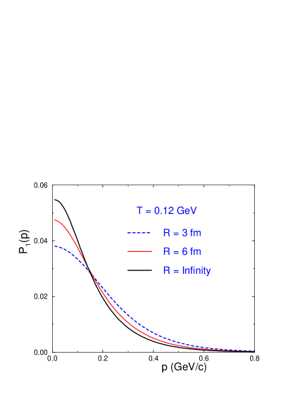
FIG. 1.: Normalized spectrum (in arbitrary units) vs. momentum $|$p$|$ (in GeV/c). The input temperature is $T=0.12$ GeV and the chemical potential is $\mu=0$. The solid line corresponds to the Bose-Einstein distribution, i.e., to the limit $R\rightarrow\infty$. The dotted and dashed lines correspond, respectively, to the $R=6$ fm and $R=3$ fm cases.

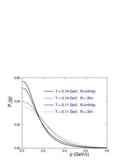
FIG. 2.: Normalized single-particle distribution (in arbitrary units) vs. momentum $|$p$|$. The input parameters are $\mu=0$, and the radius in the finite case, $R=3$ fm. The curves are shown for two values of the freeze-out temperature: $T=0.14$ GeV (solid) and $T=0.11$ GeV (dotted) and compared with the corresponding ones in the $R\rightarrow\infty$ limit.

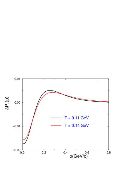
FIG. 3.: Difference in the momentum distribution (in arbitrary units), $\Delta P_{1}({\bf p})=P_{1}({\bf p})|_{R=3fm}-P_{1}({\bf p})|_{R=\infty}$, vs. $|$p$|$, of curves with $R=3$ fm and the corresponding ones in the $R\rightarrow\infty$ limit, for two values of the freeze-out temperature $T$, as indicated in the plot, with $\mu=0$.

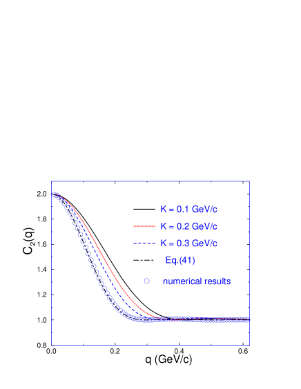
FIG. 4.: Two-pion correlation function, $C_{2}(q)$, is shown versus the momentum difference $|$q$|$=$|$${\bf p_{1}-p_{2}}$$|$. The input parameters are $T=0.12$ GeV, $R=3$ fm, and $\mu=0$. The solid, dotted, and dashed lines correspond to the average pair momentum values $K$= 0.1 GeV/c, 0.2 GeV/c, and 0.3 GeV/c, respectively. The circles refer to numerical results similar to the previous ones but with unity weight factor, $N_{\lambda}=1$, in Eq. (LABEL:pi2). The dot-dashed line corresponds to the analytical result in Eq. (41).

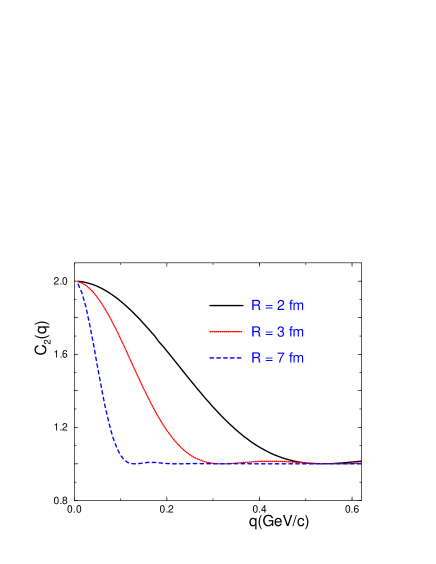
FIG. 5.: The correlation function, $C_{2}(q)$, is plotted as a function of the momentum difference, $|$q$|$=$|$${\bf p_{1}-p_{2}}$$|$. The input parameters are the temperature $T=0.12$ GeV, the average pair momentum $K=0.4$ GeV/c, and $\mu=0$. The solid, dotted, and dashed lines correspond, respectively, to the sphere radius $R$ = $2$ fm, $3$ fm, and $7$ fm.

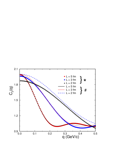
FIG. 6.: Two-pion correlation function, $C_{2}(q)$, is shown versus $|$q$|$=$|$${\bf p_{1}-p_{2}}$$|$. For helping visualization the curves are separated by brackets in two groups. In the first, signaled by ($\star$), the curves were obtained with the help of Eq. (122). The other group, signaled by ($\#$), corresponds to curves obtained by means of Eq. (126). The values adopted for the finite system sizes, i.e., $L$= $2$ fm, $3$ fm, and $5$ fm, are shown in the plot.

REFERENCES

• [1] See for example: C.Y. Wong, Introduction to high energy heavy-ion collisions, (World Scientific, Singapore, 1994); Quark-Gluon-Plasma 2, edited by R.C. Hwa ( World Scientific, Singapore, 1995).
• [2] R. Hanbury-Brown and R.Q. Twiss, Phil. Mag. 45, 663 (1954);   Nature 177, 27 (1956)   and  178, 1447 (1956).
• [3] G. Goldhaber, S. Goldhaber, W. Lee, and A. Pais, Phys. Rev. 120, 300 (1960).
• [4] for a long list of references on interferometry, see i) W.A. Zajc, Il Ciocco 1992, Particle production in highly excited matter (NATO Advanced Study Institute), p. 435, Castelvecchio Pascoli, Italy, 12-24 Jul 1992; ii) D. H. Boal, C. K. Gelbke, and B. K. Jennings, Rev. Mod. Phys. 62, 553 (1990); iii) R. M. Weiner, Bose-Einstein Correlation in Particle and Nuclear Physics, J. Wiley & Sons (1997); iv) U. Heinz and B. V. Jacak, Ann. Rev. Nucl. Part. Sci. 49, 529 (1999).
• [5] M. Gyulassy, S. Kauffmann and L. Wilson, Phys. Rev. C 20, 2267 (1979).
• [6] I. V. Andreev, M. Plümer and R.M. Weiner, Phys. Rev. Lett. 67, 3475 (1991); I. V. Andreev, M. Plümer and R. M. Weiner, Int. J. Mod. Phys. A8, 4577 (1993).
• [7] C.Y. Wong, Phys. Rev. C 43, 902 (1993).
• [8] Yu. Sinyukov, Nucl. Phys. A566, 589c (1994).
• [9] M. Mostafa and C.Y. Wong, Phys. Rev. C 51, 2135 (1995).
• [10] A. Ayala and A. Smerzi, Phys. Lett. B405, 20 (1997); A. Ayala, J. Barreiro and L. M. Montaño, Phys. Rev. C 60, 014904 (1999).
• [11] Yu. Sinyukov, nucl-th/9909018 – this reference is a version with minor modifications of the unpublished paper ITP-93-8E - Kiev (1993).
• [12] E. V. Shuryak, Phys. Rev. D 42, 1764 (1990).
• [13] S. Pratt, Phys. Rev. Lett. 53, 1219 (1984).
• [14] S. S. Padula, M. Gyulassy, and S. Gavin, Nucl. Phys. B329, 357 (1990).
• [15] U. Heinz, in Correlations and Clustering Phenomena in Subatomic Physics, edited by M.N. Harakeh et al., p. 137 (Plenum, New York, 1997).
• [16] S. Sarkar, P. K. Roy, D. K. Srivastava, and B. Sinha, J. Phys. G22, 951 (1996).
• [17] It was shown in Ref.[5] that, since for a point-like source we have only one emitter, the corresponding pion multiplicity distribution is Poisson and the two-pion correlation function is 1.
Refer to caption