Nucleon form factors and a nonpointlike diquark

Abstract

Nucleon form factors are calculated on $q^{2}\in[0,3]\,$GeV² using an Ansatz for the nucleon’s Fadde’ev amplitude motivated by quark-diquark solutions of the relativistic Fadde’ev equation. Only the scalar diquark is retained, and it and the quark are confined. A good description of the data requires a nonpointlike diquark correlation with an electromagnetic radius of $0.8\,r_{\pi}$. The composite, nonpointlike nature of the diquark is crucial. It provides for diquark-breakup terms that are of greater importance than the diquark photon absorption contribution.

Mesons present a two-body problem, and the Dyson-Schwinger equations (DSEs) have been widely used in the calculation of their properties and interactions [1, 2]. Many studies have focused on electromagnetic processes; such as the form factors of light pseudoscalar [3, 4] and vector mesons [5], and the $\gamma^{\ast}\pi^{0}\to\gamma$ [6, 7, 8], $\gamma^{\ast}\pi\to\rho$ [7] and $\gamma\pi^{\ast}\to\pi\pi$ [9] transition form factors, all of which are accessible at TJNAF. These studies provide a foundation for the exploration of nucleons, which is fundamentally a three-body problem.

The nucleon’s bound state amplitude can be obtained from a relativistic Fadde’ev equation [10]. Its analysis may be simplified by using the feature that ladder-like dressed-gluon exchange between quarks is attractive in the colour antitriplet channel. Then, in what is an analogue of the rainbow-ladder truncation for mesons, the Fadde’ev equation can be reduced to a sum of three coupled equations, in which the primary dynamical content is dressed-gluon exchange generating a correlation between two quarks and the iterated exchange of roles between the dormant and diquark-participant quarks. Following this approach, the diquark correlation is represented by the solution of an homogeneous Bethe-Salpeter equation in the dressed-ladder truncation and hence its contribution to the quark-quark scattering matrix, ${\cal M}_{qq}$, is that of an asymptotic bound state; i.e., it contributes a simple pole. That is an artefact of the ladder truncation [11] and complicates solving the Fadde’ev equation [12] by introducing spurious free-particle singularities in the kernel.

Studies of DSE-models [1, 2] suggest that confinement can be realised via the absence of a Lehmann representation for coloured Green functions, and have led to a phenomenologically efficacious parametrisation of the dressed-quark Schwinger function [3]. A similar parametrisation of the diquark contribution to ${\cal M}_{qq}$, advocated in Ref. [13], has been used to good effect in solving the Fadde’ev equation [14]. We use such representations herein.

The nucleon-photon current is

$$J_{\mu}(P^{\prime},P) = ie\,\bar{u}(P^{\prime})\,\Lambda_{\mu}(q,P)\,u(P)\,,$$ (1)

where the spinors satisfy: $\gamma\cdot P\,u(P)=iMu(P)$, $\bar{u}(P)\,\gamma\cdot P=iM\bar{u}(P)$, with $M=0.94\,$GeV the nucleon mass, and $q=(P^{\prime}-P)$. The complete specification of a fermion-vector-boson vertex requires twelve independent scalar functions:

$$i\Lambda_{\mu}(q,P)=i\gamma_{\mu}\,f_{1}+i\sigma_{\mu\nu}\,q_{\nu}\,f_{2}+R_{\mu}\,f_{3}+i\gamma\cdot R\,R_{\mu}\,f_{4}$$ (3)

$$+i\sigma_{\nu\rho}\,R_{\mu}\,q_{\nu}\,R_{\rho}\,f_{5}+i\gamma_{5}\gamma_{\nu}\,\varepsilon_{\mu\nu\rho\sigma}\,q_{\rho}\,R_{\sigma}\,f_{6}\,+\ldots\,,$$

where $f_{i}=f_{i}(q^{2},q\cdot P,P^{2})$, $R=(P^{\prime}+P)$ and $q\cdot R=0$ for elastic scattering. However, using the definition of the nucleon spinors, (1) can be written

$$J_{\mu}(P^{\prime},P)=$$ (5)

$$ie\,\bar{u}(P^{\prime})\left(\gamma_{\mu}\,F_{1}(q^{2})+\frac{1}{2M}\,\sigma_{\mu\nu}\,q_{\nu}\,F_{2}(q^{2})\right)u(P)\,,$$

where the Dirac and Pauli form factors are

$$F_{1}=$$ (7)

$$f_{1}+2\,M\,f_{3}-4\,M^{2}\,f_{4}-2\,M\,q^{2}\,f_{5}-q^{2}\,f_{6}\,,$$

$$F_{2}=$$ (9)

$$2\,M\,f_{2}-2\,M\,f_{3}+4\,M^{2}\,f_{4}+2\,M\,f_{5}-4\,M^{2}\,f_{6}\,,$$

in terms of which one has the electric and magnetic form factors:

$$G_{E}(q^{2}) = F_{1}(q^{2})-\frac{q^{2}}{4M^{2}}F_{2}(q^{2})\,,$$ (10)

$$G_{M}(q^{2}) = F_{1}(q^{2})+F_{2}(q^{2})\,.$$ (11)

To calculate these form factors we represent the nucleon as a three-quark bound state involving a diquark correlation, and require the photon to probe the diquark’s internal structure. Antisymmetrisation ensures there is an exchange of roles between the dormant and diquark-participant quarks and this gives rise to diquark “breakup” contributions. We describe the propagation of the dressed-quarks and diquark correlation by confining parametrisations and hence pinch singularities associated with quark production thresholds are absent. Our calculation is kindred to many studies of meson properties [3, 4, 5, 6, 7, 9].

We write the Fadde’ev amplitude of the nucleon as [15]

$$\Psi^{\tau}_{\alpha}(p_{1},\alpha_{1},\tau^{1};p_{2},\alpha_{2},\tau^{2};p_{3},\alpha_{3},\tau^{3})=$$ (13)

$$\varepsilon_{c_{1}c_{2}c_{3}}\,\delta^{\tau\tau^{3}}\,\delta_{\alpha\alpha_{3}}\,\psi(p_{1}+p_{2},p_{3})\,\Delta(p_{1}+p_{2})\,\Gamma_{\alpha_{1}\alpha_{2}}^{\tau^{1}\tau^{2}}(p_{1},p_{2})\,,$$

where $\varepsilon_{c_{1}c_{2}c_{3}}$ effects a singlet coupling of the quarks’ colour indices, $(p_{i},\alpha_{i},\tau^{i})$ denote the momentum and the Dirac and isospin indices for the $i$-th quark constituent, $\alpha$ and $\tau$ are these indices for the nucleon itself, $\psi(\ell_{1},\ell_{2})$ is a Bethe-Salpeter-like amplitude characterising the relative-momentum dependence of the correlation between diquark and quark, $\Delta(K)$ describes the propagation characteristics of the diquark, and

$$\Gamma_{\alpha_{1}\alpha_{2}}^{\tau^{1}\tau^{2}}(p_{1},p_{2}) = (Ci\gamma_{5})_{\alpha_{1}\alpha_{2}}\,(i\tau_{2})^{\tau^{1}\tau^{2}}\,\Gamma(p_{1},p_{2})$$ (14)

represents the momentum-dependence, and spin and isospin character of the diquark correlation; i.e., it corresponds to a diquark Bethe-Salpeter amplitude.

With this form of $\Psi$, we retain in ${\cal M}_{qq}$ only the contribution of the scalar diquark, which has the largest correlation length [13]: $\lambda_{0^{+}}:=1/m_{0^{+}}=0.27\,$fm. For all $(ud)$-correlations with $J^{P}\neq 1^{+}$, $\lambda_{ud}<0.5\,\lambda_{0^{+}}$. The axial-vector correlation is different: $\lambda_{1^{+}}=0.78\,\lambda_{0^{+}}$, and it is quantitatively important in the calculation of baryon masses ($\mathrel{\hbox to0.0pt{\lower 4.0pt\hbox{\hskip 0.0pt$\sim$}\hss}\raise 1.0pt\hbox{$<$}}30$%) [14]. Hence we anticipate that neglecting the $1^{+}$ correlation will prove the primary defect of our Ansatz. However, it is an helpful expedient in this exploratory calculation, which is made complicated by our desire to elucidate the effect of the diquarks’ internal structure.

Our impulse approximation to the nucleon form factor is depicted in Fig. 1. Enumerating from top to bottom, the diagrams represent

$$\Lambda^{1}_{\mu}(q,P)=3\int\!\!\mbox{$\frac{d^{4}\ell}{(2\pi)^{4}}$}\,$$ (16)

$$\psi(K,p_{3}+q)\Delta(K)\psi(K,p_{3})\,Q_{F}\Lambda_{\mu}^{q}(p_{3}+q,p_{3})\,,$$

with $K=\eta P+\ell$, $p_{3}=(1-\eta)P-\ell$, $p_{2}=K/2-k$, $Q_{F}={\rm diag}(2/3,-1/3)$, $\Lambda_{\mu}^{q}(k_{1},k_{2})=S(k_{1})\,\Gamma_{\mu}(k_{1},k_{2})\,S(k_{2})$,

$$\Lambda^{2}_{\mu}(q,P)=6\int\!\!\mbox{$\frac{d^{4}k}{(2\pi)^{4}}$}\mbox{$\frac{d^{4}\ell}{(2\pi)^{4}}$}\,\Omega(p_{1}+q,p_{2},p_{3})\,$$ (18)

$$\times\Omega(p_{1},p_{2},p_{3})\,{\rm tr}_{D}\left[\Lambda_{\mu}^{q}(p_{1}+q,p_{1})S(p_{2})\right]\,S(p_{3})\,\mbox{$\frac{1}{3}$}I_{F}\,,$$

which contributes equally to the proton and neutron and contains the diquark electromagnetic form factor, with $6=\varepsilon_{c_{1}c_{2}c_{3}}\varepsilon_{c_{1}c_{2}c_{3}}$ and

$$\Omega(p_{1},p_{2},p_{3})=\psi(p_{1}+p_{2},p_{3})\,\Delta(p_{1}+p_{2})\,\Gamma(p_{1},p_{2})\,,$$ (19)

$$\Lambda^{3}_{\mu}(q,P)=6\int\!\!\mbox{$\frac{d^{4}k}{(2\pi)^{4}}$}\mbox{$\frac{d^{4}\ell}{(2\pi)^{4}}$}\,\Omega(p_{1}+q,p_{3},p_{2})\,$$ (21)

$$\times\Omega(p_{1},p_{2},p_{3})\,S(p_{2})\,(i\tau_{2})^{\rm T}Q_{F}(i\tau_{2})\,\Lambda^{q}_{\mu}(p_{1},p_{1}+q)\,S(p_{3})\,,$$

$$\Lambda^{4}_{\mu}(q,P)=6\int\mbox{$\frac{d^{4}k}{(2\pi)^{4}}$}\mbox{$\frac{d^{4}\ell}{(2\pi)^{4}}$}\,\Omega(p_{1},p_{3},p_{2}+q)\,$$ (23)

$$\times\Omega(p_{1},p_{2},p_{3})\,Q_{F}\Lambda^{q}_{\mu}(p_{2}+q,p_{2})\,S(p_{1})\,S(p_{3})\,,$$

$$\Lambda^{5}_{\mu}(q,P)=6\int\mbox{$\frac{d^{4}k}{(2\pi)^{4}}$}\mbox{$\frac{d^{4}\ell}{(2\pi)^{4}}$}\,\Omega(p_{1},p_{3}+q,p_{2})\,$$ (25)

$$\times\Omega(p_{1},p_{2},p_{3})\,S(p_{2})\,S(p_{1})\,Q_{F}\Lambda_{\mu}(p_{3}+q,p_{3})\,.$$

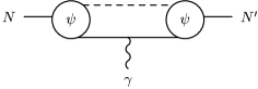
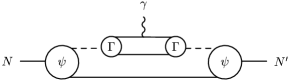
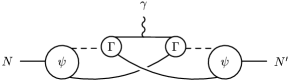
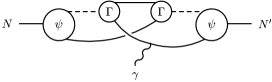
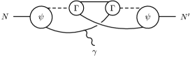
FIG. 1.: Our impulse approximation to the electromagnetic current requires the calculation of five contributions, (16) – (25). $\psi$: $\psi(\ell_{1},\ell_{2})$ in (13); $\Gamma$: Bethe-Salpeter-like diquark amplitude in (14); solid line: $S(q)$, quark propagator in (27); dotted line: $\Delta(K)$, diquark propagator in (40). The lowest three diagrams, which describe the interchange between the dormant quark and the diquark participants, effect the antisymmetrisation of the nucleon’s Fadde’ev amplitude. Current conservation follows because the photon-quark vertex is dressed, given in (37).

The nucleon-photon vertex is

$$\Lambda_{\mu}(q,P) = \Lambda^{1}_{\mu}(q,P)+2\sum_{i=2}^{5}\,\Lambda^{i}_{\mu}(q,P)\,.$$ (26)

(26) is fully defined once $\Psi\sim\psi\,\Gamma\,\Delta$, $S$ and $\Gamma_{\mu}$ are specified. $S$ and $\Gamma_{\mu}$ are primary elements in studies of meson properties and are already well constrained. For the dressed-quark propagator:

$$S(p) = -i\gamma\cdot p\,\sigma_{V}(p^{2})+\sigma_{S}(p^{2})$$ (27)

$$= \left[i\gamma\cdot p\,A(p^{2})+B(p^{2})\right]^{-1}\,,$$ (28)

we use the algebraic parametrisations [3]:

$$\bar{\sigma}_{S}(x) = 2\,\bar{m}\,{\cal F}(2(x+\bar{m}^{2}))$$ (30)

$$+{\cal F}(b_{1}x)\,{\cal F}(b_{3}x)\,\left[b_{0}+b_{2}{\cal F}(\epsilon x)\right]\,,$$

$$\bar{\sigma}_{V}(x) = \frac{1}{x+\bar{m}^{2}}\,\left[1-{\cal F}(2(x+\bar{m}^{2}))\right]\,,$$ (31)

with ${\cal F}(y)=(1-{\rm e}^{-y})/y$, $x=p^{2}/\lambda^{2}$, $\bar{m}$ = $m/\lambda$, $\bar{\sigma}_{S}(x)=\lambda\,\sigma_{S}(p^{2})$ and $\bar{\sigma}_{V}(x)=\lambda^{2}\,\sigma_{V}(p^{2})$. The mass-scale, $\lambda=0.566\,$GeV, and parameter values

$$\begin{array}[]{ccccc}\bar{m}&b_{0}&b_{1}&b_{2}&b_{3}\\ \hline\cr 0.00897&0.131&2.90&0.603&0.185\;\;,\end{array}$$ (32)

were fixed in a least-squares fit to light-meson observables. ($\epsilon=10^{-4}$ in (30) acts only to decouple the large- and intermediate-$p^{2}$ domains.) This algebraic parametrisation combines the effects of confinement and DCSB with free-particle behaviour at large spacelike $p^{2}$ [2].

In (16)–(25), $\Gamma_{\mu}$ is the dressed-quark-photon vertex. It satisfies the vector Ward-Takahashi identity:

$$(\ell_{1}-\ell_{2})_{\mu}\,i\Gamma_{\mu}(\ell_{1},\ell_{2})=S^{-1}(\ell_{1})-S^{-1}(\ell_{2})\,,$$ (33)

which ensures current conservation [3]. $\Gamma_{\mu}$ has been much studied [16] and, although its exact form remains unknown, its qualitative features have been elucidated so that a phenomenologically efficacious Ansatz has emerged [17]:

$$i\Gamma_{\mu}(\ell_{1},\ell_{2})=i\Sigma_{A}(\ell_{1}^{2},\ell_{2}^{2})\,\gamma_{\mu}$$ (37)

$$+(\ell_{1}+\ell_{2})_{\mu}\,\left[\mbox{$\frac{1}{2}$}i\gamma\cdot(\ell_{1}+\ell_{2})\,\Delta_{A}(\ell_{1}^{2},\ell_{2}^{2})+\Delta_{B}(\ell_{1}^{2},\ell_{2}^{2})\right]\,;$$

$$\Sigma_{F}(\ell_{1}^{2},\ell_{2}^{2})=\mbox{$\frac{1}{2}$}\,[F(\ell_{1}^{2})+F(\ell_{2}^{2})]\,,$$

$$\Delta_{F}(\ell_{1}^{2},\ell_{2}^{2})=\frac{F(\ell_{1}^{2})-F(\ell_{2}^{2})}{\ell_{1}^{2}-\ell_{2}^{2}}\,,$$

where $F=A,B$; i.e., the scalar functions in (27). A feature of (37) is that $\Gamma_{\mu}$ is completely determined by the dressed-quark propagator. Further, we estimate that calculable improvements would modify our results by $\mathrel{\hbox to0.0pt{\lower 4.0pt\hbox{\hskip 0.0pt$\sim$}\hss}\raise 1.0pt\hbox{$<$}}15\,$% [18].

The new element herein is the model of the nucleon’s Fadde’ev amplitude, (13). For the Bethe-Salpeter-like amplitudes we use the one-parameter model forms

$$\Gamma(q_{1},q_{2}) = \frac{1}{{\cal N}_{\Gamma}}\,{\cal F}(q^{2}/\omega_{\Gamma}^{2})\,,\;q:=\mbox{$\frac{1}{2}$}(q_{1}-q_{2})$$ (38)

$$\psi(\ell_{1},\ell_{2}) = \frac{1}{{\cal N}_{\Psi}}\,{\cal F}(\ell^{2}/\omega_{\psi}^{2})\,,\;\ell:=(1-\eta)\,\ell_{1}-\eta\,\ell_{2}\,.$$ (39)

Our impulse approximation is founded on a dressed-ladder kernel in the Fadde’ev equation and $\Gamma_{\mu}$ satisfies (33). Hence, the canonical normalisation conditions for the diquark and nucleon amplitudes translate to the constraints that the $(ud)$-diquark must have charge $1/3$ and the proton unit charge, which fix ${\cal N}_{\Gamma}$ and ${\cal N}_{\Psi}$. For the diquark propagator we use the one-parameter form

$$\Delta(K^{2})=\frac{1}{m_{\Delta}^{2}}\,{\cal F}(K^{2}/\omega_{\Gamma}^{2})\,,$$ (40)

and interpret $1/m_{\Delta}$ as the diquark correlation length.

We fix the model’s three parameters by optimising a fit to $G^{p}_{E}(q^{2})$ and ensuring $G_{E}^{n}(0)=0$, which yields

$$\begin{array}[]{l|ccc}&\;\omega_{\psi}&\omega_{\Gamma}&m_{\Delta}\\ \hline\cr\eta=2/3&\;0.20&1.0&0.63\end{array}$$ (41)

all in GeV ($1/m_{\Delta}=0.31\,$fm). Using Monte-Carlo methods to evaluate the multi-dimensional integrals, these values give

$$\begin{array}[]{l|c|cc}&{\rm emp.}&{\rm calc.}\\ \hline\cr r_{p}^{2}\,({\rm fm})^{2}&(0.87)^{2}&(0.79)^{2}\\ r_{n}^{2}\,({\rm fm})^{2}&-(0.34)^{2}&-(0.43)^{2}\\ \mu_{p}\,(\mu_{N})&2.79&2.88\\ \mu_{n}\,(\mu_{N})&-1.91&-1.58\\ \mu_{n}/\mu_{p}&-0.68&-0.55\end{array}$$ (42)

where the statistical error is $\mathrel{\hbox to0.0pt{\lower 4.0pt\hbox{\hskip 0.0pt$\sim$}\hss}\raise 1.0pt\hbox{$<$}}1\,$%. The sensitivity of our results to the model’s parameters is illustrated in Table I. It is clear that the fit is stable but does not bracket the experimental domain; i.e., the model lacks a relevant degree of freedom, a defect we expect including an axial-vector diquark to ameliorate.

The charge radii are obtained via

$$r_{p,n}^{2} = -6\left.\frac{d}{dq^{2}}\,F_{1}^{p,n}(q^{2})\right|_{q^{2}=0}+\frac{3}{2M^{2}}F_{2}^{p,n}(0)\,,$$ (43)

$$:= (r^{I}_{p,n})^{2}+(r^{F}_{p,n})^{2}$$ (44)

and in this calculation (in fm²)

$$\begin{array}[]{ll}(r_{p}^{I})^{2}=\;\;\,(0.70)^{2}\,,&(r_{p}^{F})^{2}=\;\;\,(0.35)^{2}\,,\\ (r_{n}^{I})^{2}=-(0.29)^{2}\,,&(r_{n}^{F})^{2}=-(0.32)^{2}\,.\end{array}$$ (45)

A $20$% reduction in $\omega_{\Gamma}$ (Table I, row 4) reduces $|r_{n}|$ by $7$%. However, that results from a $21$% reduction in $|r_{n}^{I}|$ and $2$% increase in $|r_{n}^{F}|$. We attribute our overestimate of $|r_{n}^{2}|$ to a poor description of $F_{1}^{n}(q^{2})$, which involves many cancellations between terms because of the $(u,d,d)$ electric charge combinations and must vanish at $q^{2}=0$.

Five diagrams contribute to our impulse approximation and diagram 2 involves the diquark form factor. The calculated value of the associated elastic charge radius provides a measure of the size of the “constituent” diquark:

$$r_{\rm 0^{+}}^{2} = (0.45\,{\rm fm})^{2}=(0.80\,r_{\pi})^{2}\,,$$ (46)

with $r_{\pi}$ calculated in the same model [3], and in quantitative agreement with another estimate [22]. This is important because, with $\omega_{\Gamma}$ allowed to vary, $r_{0^{+}}$ is a qualitative prediction of the model. Thus an optimal description of the data requires a nonpointlike diquark.

Table II provides a guide to each diagram’s relative importance. In all cases the first diagram, describing scattering from the dormant quark, is the most significant. For the charge radii the breakup contributions are comparable in magnitude to the second diagram, photon-diquark scattering. The magnetic moments are of particular interest. A scalar diquark does not have a magnetic moment, and that is expressed in our calculation by the very small contribution from diagram $2$. It is not identically zero because of the confinement of the spectator quark; i.e., the absence of a mass-shell. Diagrams $3$-$5$ only appear because the diquark is a nonpointlike composite and they provide $\sim 50\,$% of $\mu_{p}$, $\mu_{n}$. Discarding these contributions one obtains $\mu_{n}/\mu_{p}\geq-0.5$, and in pointlike diquark models the axial-vector has alone been forced to remedy that defect [23]. Our results indicate that approach to be erroneous, attributing too much importance to the axial-vector correlation.

The calculated form factors are depicted in Figs. 2 and 3 and it is obvious in Fig. 2 that we used $G_{E}^{p}(q^{2})$ to constrain our fit. The $0^{+}$ $(ud)$ diquark correlation in $\Psi$ ensures that $G_{E\,{\rm fit}}^{n}(q^{2})\not\equiv 0$, and the presence of diquark correlations can also explain the $N$-$\Delta$ mass difference. Our result for $G_{E}^{n}(q^{2})$ is well described by [20]

$$G_{E\,{\rm fit}}^{n}(q^{2})=-\mu_{n}^{\rm emp}\,F_{\rm emp}(q^{2})\,\frac{a^{2}\,\tau}{1+b^{2}\,\tau}\,,$$ (47)

with $\tau=q^{2}/(2M)^{2}$, $F_{\rm emp}(q^{2})$ given in Fig. 2, and $a=1.33$, $b=1.00$, and the discrepancy between our calculation and experiment can be discussed in terms of these parameters. $a$ characterises the charge radius and it is $\mathrel{\hbox to0.0pt{\lower 4.0pt\hbox{\hskip 0.0pt$\sim$}\hss}\raise 1.0pt\hbox{$<$}}30$% too large, as can be anticipated from (42). $b$ describes the magnitude at intermediate momenta and it is only $\sim 23$-$35$% of the empirical value. That is a systematic defect shared by other studies [24] that only retain the scalar diquark correlation. Unlike those studies, however, our calculated magnetic form factors, Fig 3, agree well with the data and, as we have seen, that is because we include the diquark breakup diagrams.

TABLE I.: A variation of the model parameters: $\omega_{\psi}$, $\omega_{\Gamma}$ and $m_{\Delta}$ (in GeV) illustrates the sensitivity and stability of our results. The column labelled “$r_{n}$” lists: ${\rm sign}(r_{n}^{2})\,|r_{n}^{2}|^{1/2}$. (Radii in fm, magnetic moments in units of $\mu_{N}$. The statistical errors are $\leq 1$%.)

$\displaystyle\begin{array}[]{ccc|ccccc}\hline\cr\omega_{\psi}&\omega_{\Gamma}&m_{\Delta}&r_{p}&r_{n}&\mu_{p}&\mu_{n}&\mu_{n}/\mu_{p}\\ \hline\cr 0.20&1.0&0.63&0.79&-0.43&2.88&-1.58&-0.55\\ \hline\cr 0.16&1.0&0.63&0.84&-0.46&2.83&-1.55&-0.55\\ 0.24&1.0&0.62&0.75&-0.41&2.89&-1.59&-0.55\\ \hline\cr 0.20&0.8&0.62&0.80&-0.40&2.93&-1.64&-0.56\\ 0.20&1.2&0.63&0.78&-0.45&2.84&-1.54&-0.54\\ \hline\cr\end{array}$

FIG. 2.: Upper panel: Calculated proton electric form factor: $+$, compared with the empirical dipole fit: $F_{\rm emp}(q^{2})=1/(1+q^{2}/m^{2}_{\rm emp})^{2}$, $m_{\rm emp}=0.84\,$GeV. Lower panel: Calculated neutron electric form factor: $+$, compared with the experimental data [20] as extracted using the Argonne V18 potential [21]. In both calculations the Monte-Carlo errors are smaller than the symbols.

It must be borne in mind that in our calculation $a$ and $b$ are not independent. Modifying the parameters in (41) so as to reduce $a$ automatically and substantially increases $b$. However, not withstanding our observation that its importance has previously been overestimated, without an axial-vector diquark correlation it is not possible to accurately describe all observables simultaneously.

We have employed a three-parameter model of the nucleon’s Fadde’ev amplitude, $\Psi$, to calculate an impulse approximation to the electromagnetic form factors. $\Psi$ represents the nucleon as a bound state of a confined quark and confined, nonpointlike scalar diquark, and the exchange of roles between the dormant and diquark-participant quarks is an integral feature. Five processes contribute: direct quark-photon scattering with a spectator diquark; photon-diquark scattering with a spectator quark; and three distinct diquark breakup diagrams. We obtain a good description of all form factors except $G_{E}^{n}$, which is too large in magnitude. That defect is shared by all models that do not include more than a scalar diquark correlation. The nonpointlike nature of the diquark correlation is important, especially via the breakup contributions which provide large contributions to the magnetic moments and ensure $\mu_{n}/\mu_{p}<-0.5$.

FIG. 3.: Calculated proton and neutron magnetic form factors, normalised by $|\mu_{p,n}|$ in (42). The curves are dipole fits with masses (in GeV): $m_{p}=0.95$, $m_{n}=1.0$, $13$% and $19$% larger than $m_{\rm emp}$ in Fig. 2. ($\mu^{\rm emp}_{p,n}\,F_{\rm emp}(q^{2})$ describes the data very well.)

Including a nonpointlike axial-vector diquark is an obvious improvement of the model. That must be done in analogy with the scalar diquark because an accurate interpretation of the model parameters is impossible if the breakup diagrams are discarded. Another avenue for improvement is a direct solution of the Fadde’ev equation, retaining the axial-vector correlation and the breakup contributions to the form factor. That would provide a model for correlating meson and baryon observables in terms of very few parameters.

Models of the nucleon such as ours have hitherto been applied only at small- and intermediate-$q^{2}$. Based on the observation [4] that a description of the large-$q^{2}$ behaviour of $F_{\pi}(q^{2})$ is only possible if the subleading pseudovector components of the pion’s Bethe-Salpeter amplitude are retained, we anticipate that a successful description of the nucleon form factors on that domain will require a parametrisation of the Fadde’ev amplitude that includes the analogous subleading Dirac components.

TABLE II.: Relative contribution to the charge radii and magnetic moments of each of the five diagrams in our impulse approximation: Fig. (1), (16)–(25).

$\displaystyle\begin{array}[]{r|rrrrr}\hline\cr{\rm diagram}&1&2&3&4&5\\ \hline\cr(r_{p}^{2})^{i}/r_{p}^{2}&\;0.68&0.11&-0.02&0.12&0.12\\ (r_{n}^{2})^{i}/r_{n}^{2}&\;1.14&-0.37&-0.15&0.19&0.19\\ \mu_{p}^{i}/\mu_{p}&\;0.60&0.01&0.04&0.17&0.17\\ \mu_{n}^{i}/\mu_{n}&\;0.55&-0.02&0.15&0.16&0.16\\ \hline\cr\end{array}$

This work was supported by the US Department of Energy, Nuclear Physics Division, under contract number W-31-109-ENG-38. S.M.S. is a F.-Lynen Fellow of the A.v. Humboldt foundation.

REFERENCES

• [1] C.D. Roberts and A.G. Williams, Prog. Part. Nucl. Phys. 33 (1994) 477.
• [2] C.D. Roberts, Fiz. Élem. Chastits At. Yadra 30 (1999) 537 (Phys. Part. Nucl. 30 (1999) 223).
• [3] C.J. Burden, C.D. Roberts and M.J. Thomson, Phys. Lett. B371 (1996) 163.
• [4] P. Maris and C.D. Roberts, Phys. Rev. C58 (1998) 3659.
• [5] F.T. Hawes and M.A. Pichowsky, Phys. Rev. C59 (1999) 1743.
• [6] C.D. Roberts, “Dyson Schwinger equations: Connecting small and large length scales,” nucl-th/9901091.
• [7] P.C. Tandy, “Electromagnetic form-factors of meson transitions,” hep-ph/9902459.
• [8] D. Klabu$\check{\rm c}$ar and D. Kekez, “Schwinger-Dyson approach and generalized impulse approximation for the $\pi^{0}\to\gamma^{\ast}\gamma$ transition,” hep-ph/9905251.
• [9] R. Alkofer and C.D. Roberts, Phys. Lett. B369 (1996) 101.
• [10] R.T. Cahill, C.D. Roberts and J. Praschifka, Austral. J. Phys. 42 (1989) 129.
• [11] A. Bender, C.D. Roberts and L. Von Smekal, Phys. Lett. B380 (1996) 7.
• [12] C.J. Burden, R.T. Cahill and J. Praschifka, Austral. J. Phys. 42 (1989) 147.
• [13] C.J. Burden, L. Qian, C.D. Roberts, P.C. Tandy and M.J. Thomson, Phys. Rev. C55 (1997) 2649.
• [14] M. Oettel, G. Hellstern, R. Alkofer and H. Reinhardt, Phys. Rev. C58 (1998) 2459.
• [15] A. Bender, “Probing Confined-Quark Dynamics via Nucleon Form Factors”, in Proceedings of the 14th International Conference on Particles and Nuclei, edited by C.E. Carlson and J.J. Domingo (World Scientific, Singapore, 1997), pp. 669-670.
• [16] A. Bashir, A. Kizilersu and M.R. Pennington, Phys. Rev. D57 (1998) 1242.
• [17] J.S. Ball and T. Chiu, Phys. Rev. D22 (1980) 2542.
• [18] R. Alkofer, A. Bender and C.D. Roberts, Int. J. Mod. Phys. A10 (1995) 3319.
• [19] P. Maris and C.D. Roberts, Phys. Rev. C56 (1997) 3369.
• [20] S. Platchkov et al., Nucl. Phys. A510 (1990) 740.
• [21] R.B. Wiringa, private communication; R.B. Wiringa, V.G. Stoks and R. Schiavilla, Phys. Rev. C51 (1995) 38.
• [22] C. Weiss, A. Buck, R. Alkofer and H. Reinhardt, Phys. Lett. B312 (1993) 6.
• [23] V. Keiner, Phys. Rev. C54 (1996) 3232.
• [24] G.V. Efimov, M.A. Ivanov and V.E. Lyubovitsky, Z. Phys. C47 (1990) 583; V. Keiner, Z. Phys. A354 (1996) 87; G. Hellstern, R. Alkofer, M. Oettel and H. Reinhardt, Nucl. Phys. A627 (1997) 679.