Quasifree Kaon Photoproduction on Nuclei

Abstract

Investigations of the quasifree reaction A$(\gamma,KY)$B are presented in the distorted wave impulse approximation (DWIA). For this purpose, we present a revised tree-level model of elementary kaon photoproduction that incorporates hadronic form factors consistent with gauge invariance, uses SU(3) values for the Born couplings and uses resonances consistent with multi-channel analyses. The potential of exclusive quasifree kaon photoproduction on nuclei to reveal details of the hyperon-nucleus interaction is examined. Detailed predictions for the coincidence cross section, the photon asymmetry, and the hyperon polarization and their sensitivities to the ingredients of the model are obtained for all six production channels. Under selected kinematics these observables are found to be sensitive to the hyperon-nucleus final state interaction. Some polarization observables are found to be insensitive to distortion effects, making them ideal tools to search for possible medium modifications of the elementary amplitude.

I Introduction

With the start of experimental activities at Jefferson Lab and other continuous beam electron accelerators with sufficient energy and intensity, explorations in hypernuclear physics through electromagnetic probes are becoming a reality. The use of kaon photoproduction to excite discrete hypernuclear states through the reaction A$(\gamma,K)_{Y}$B has been investigated extensively [1, 2, 3, 4]. This reaction involves high momentum transfers to the residual nucleus, resulting in a cross section that is suppressed by nuclear form factors, and sensitive to the details of hypernuclear transition densities. The probability of forming such bound states is in fact rather small. It was estimated [2] that this formation probability is around 5-10% of the total $(\gamma,K^{+})$ strength on nuclear targets. Thus, most of the kaon production events will come from quasifree production.

In this work, we present theoretical predictions for exclusive quasifree kaon photoproduction, A$(\gamma,KY)$B, in a Distorted Wave Impulse Approximation (DWIA) framework. This reaction allows for the study of the production process in the nuclear medium as well as final state interaction (FSI) effects without being obscured by the details of the nuclear transition. This is due mainly to the quasifree nature of the reaction which permits the kinematic flexibility to have small momentum transfers. Conceptually, the initial nucleus is a target holder which presents a bound nucleon to the incoming photon beam. The basic reaction $N(\gamma,KY)$ takes place in the nuclear medium producing a continuum kaon and hyperon which interact with the residual nucleus as they exit the target.

The purpose of the present study is two fold: First, we want to examine the sensitivity of various observables to the hyperon-nucleus final-state interaction. The study of the Y-nucleus potential permits access to the $YN$ interaction, which is much less well-known than the $\pi N$ and $NN$ interactions. This is mainly due to lack of hyperon beams in accelerator experiments. Recently, effective field theories (EFTs) have been successfully applied to the strong two-nucleon sector [5]. While the use of EFTs in the SU(2) regime is now well-established, their range of applicability to SU(3) is much less certain due to the much larger degree of SU(3) symmetry breaking. In order to assess the validity of EFTs in SU(3) a good phenomenological understanding of the $YN$ force is required. At present, much of our knowledge on the $YN$ interaction is based on studies of hypernuclei formed in hadronic reactions such as $(K^{-},\pi^{-})$ and $(\pi^{+},K^{+})$ [6, 7].

The second goal of this study is to establish the kinematic range within which polarization observables are insensitive to distortion effects. This would allow a clearer signal for possible medium modifications of the elementary operator to emerge, as suggested in Ref. [8]. One aspect of this investigation is the puzzle of the ”damped resonances” in the second and third resonance regions as seen in inclusive photoabsorption cross section data on various nuclei [9]. The data show an unexpected damping behavior of the higher resonances when compared with the same process on the proton and the deuteron. In order to isolate the mechanism for this mysterious phenomenon the individual exclusive channels need to be investigated. In Ref. [8], the authors - using PWIA - demonstrate the sensitivity of polarization observables to the elementary amplitude, while on the other hand they find these observables to be insensitive to relativistic effects or the specific nuclear target. In this study, we compare DWIA with PWIA calculations over a wide kinematic range and thus establish the range of validity for the conclusions drawn in Ref. [8]. Experimentally, there is already an approved Jefferson Lab proposal for Hall B [10] to measure this reaction.

The key ingredients in quasifree kaon photoproduction on nuclei are: a) the single-particle wave function of the initial nucleon and spectroscopic factor, usually taken from electron scattering, b) the elementary kaon photoproduction amplitude, obtained from models of the free processes, c) the distorted kaon wave function, and finally, d) the hyperon-nucleus final state interaction. This framework has been applied in our previous works for pion photo- and electro-production [11] and eta photoproduction [12] from nuclei, and was found to give a good description of the experimental data. This previous agreement with experiment partially justifies the impulse approximation implicit in the model outlined above that we will use in our analysis. Preliminary results in this work have been presented in a conference talk [13].

This paper is organized as follows. In Sec. II we discuss the revised elementary operator and compare it to the currently available experimental data of kaon photoproduction on the nucleon. Section III outlines the key ingredients in the DWIA model. Section IV reports our calculations under two different kinematic arrangements. Section V contains our concluding remarks.

II The Elementary Photoproduction Amplitude

While dynamical models involving various approximations for the Bethe-Salpeter equation are becoming increasingly successful in the description of pion photoproduction, the hadronic final state interaction in kaon photoproduction has usually been left out [14, 15, 16, 17]. Neglecting the final meson-baryon interaction in the full meson photoproduction $T$-matrix automatically leads to violation of unitarity since flux going into inelastic channels has not been properly accounted for. Enforcing unitarity dynamically requires solving a system of coupled channels with all possible final states. In the case of $K^{+}\Lambda$ photoproduction, this arduous task has recently been accomplished by Feuster and Mosel [18, 19] using a K-matrix approach. However, such an amplitude is rather cumbersome to use in reactions on nuclei. For our purpose, we therefore follow older models[14, 15, 16, 17] and choose an isobaric model without final-state interactions which provides a simple tool to parameterize meson photoproduction off the nucleon. Without rescattering contributions the $T$-matrix is simply approximated by the driving term alone which is assumed to be given by a series of tree-level diagrams. The selected Feynman diagrams for the $s$-, $u$-, and $t$-channel contain some unknown coupling parameters to be adjusted in order to reproduce experimental data. Final state interaction is effectively absorbed in these coupling constants which then cannot easily be compared to couplings from other reactions.

One of the most contentious issues in the phenomenological description of kaon photoproduction on the nucleon has been the choice of baryon resonances in the production amplitude [14, 15, 16, 19, 20]. Many authors have selected resonances that contribute to the kaon production process by their relative contribution to the overall $\chi^{2}$ of the fit [14, 15, 20]. Our approach here is different: we wish to construct an amplitude with a ”minimal” number of resonances that is easy to handle in the nuclear context. We use the results of recent multichannel analyses [18, 19, 21, 22] as a guide to inform us of the most important resonances that decay into $K\Lambda$ and $K\Sigma$ final states with a significant branching ratio. Thus, in contrast to Refs. [14, 20], we do not include spin 5/2 states in our amplitude since neither coupled-channels results nor older partial-wave analyses[23, 24] find their contributions to be important. Ultimately, only a multipole analysis will be able to clearly identify the resonances participating in kaon photoproduction. Using input from the multichannel calculations by Refs. [18, 19, 21, 22] we include the three resonances that have been found to decay noticeably into the $K\Lambda$ channel: $S_{11}$(1650), $P_{11}$(1710), and $P_{13}(1720)$. For $K\Sigma$ production we also allow contributions from the $S_{31}$(1900) and $P_{31}$(1910) resonances. Furthermore, we include not only the usual $1^{-}$ vector meson $K^{*}(892)$, but also the $1^{+}$ pseudovector meson $K_{1}(1270)$ in the $t$-channel since a number of studies [14, 15, 25] have found this resonance to give a significant contribution.

A Isospin Symmetry and Resonance Terms

Following Refs.[26, 27, 28] we write the transition matrix of the reaction

$$\gamma(p_{\gamma})+N(p_{N})\longrightarrow K(p_{K})+Y(p_{Y})$$ (1)

which stands for the following six reaction channels

$$\gamma+p \rightarrow K^{+}+\Lambda,$$ (2)

$$\gamma+p \rightarrow K^{+}+\Sigma^{0},$$ (3)

$$\gamma+p \rightarrow K^{0}+\Sigma^{+},$$ (4)

$$\gamma+n \rightarrow K^{0}+\Lambda,$$ (5)

$$\gamma+n \rightarrow K^{+}+\Sigma^{-},$$ (6)

$$\gamma+n \rightarrow K^{0}+\Sigma^{0}.$$ (7)

in the form of

$$M_{\mathrm{f}i} = {\bar{u}}({\mbox{\boldmath${p}$}}_{Y},s_{Y})\sum_{i=1}^{4}A_{i}~{}M_{i}~{}u({\mbox{\boldmath${p}$}}_{N},s_{N})~{},$$ (8)

where the Lorentz invariant matrices $M_{i}$ are given by

$$M_{1} = \gamma_{5}~{}\epsilon\!\!/p_{\gamma}\!\!\!\!\!/~{}~{},$$ (9)

$$M_{2} = 2\gamma_{5}(p_{K}\cdot\epsilon~{}p_{N}\cdot p_{\gamma}-p_{K}\cdot p_{\gamma}~{}p_{N}\cdot\epsilon)~{},$$ (10)

$$M_{3} = \gamma_{5}(p_{K}\cdot p_{\gamma}~{}\epsilon\!\!/-p_{K}\cdot\epsilon~{}p_{\gamma}\!\!\!\!\!/~{})~{},$$ (11)

$$M_{4} = i\epsilon_{\mu\nu\rho\sigma}\gamma^{\mu}p_{K}^{\nu}\epsilon^{\rho}p_{\gamma}^{\sigma}~{}.$$ (12)

The amplitudes $A_{i}$ are obtained from the Feynman diagrams of Fig. 1 by using the vertex factors and the propagators given in Ref. [29, 30]. Casting the elementary operator in the above form is convenient since it assures gauge invariance even in the case of bound nucleons that the amplitude operates on inside the nucleus in the framework of the impulse approximation.

To relate the hadronic coupling constants among the various isospin channels we use isospin symmetry

$$g_{K^{+}\Lambda p} = g_{K^{0}\Lambda n}~{},$$ (13)

$$g_{K^{+}\Sigma^{0}p} = -g_{K^{0}\Sigma^{0}n}=g_{K^{0}\Sigma^{+}p}/\sqrt{2}=g_{K^{+}\Sigma^{-}n}/\sqrt{2}~{},$$ (14)

$$g_{K^{+}\Sigma^{0}\Delta^{+}} = g_{K^{0}\Sigma^{0}\Delta^{0}}~{}=~{}-\sqrt{2}g_{K^{0}\Sigma^{+}\Delta^{+}}~{}=~{}\sqrt{2}g_{K^{+}\Sigma^{-}\Delta^{0}}~{}.$$ (15)

The electromagnetic couplings of the resonances to the proton and the neutron can be related by means of helicity amplitudes. Following Ref. [19] we can write the helicity amplitude of spin 1/2 resonances in terms of their coupling constants as

$$A_{1/2}^{(\pm)} = \mp\frac{1}{2m_{N}}\left(\frac{m_{N^{*}}^{2}-m_{N}^{2}}{2m_{N}}\right)^{1/2}~{}eg_{N^{*}N\gamma}~{},$$ (16)

where the sign refers to the resonance parity of the resonance. Therefore, the relation between spin 1/2 coupling constants for the production on the proton and on the neutron is given by

$$\frac{g_{N^{*0}n\gamma}}{g_{N^{*+}p\gamma}} = \frac{A_{1/2}^{n}}{A_{1/2}^{p}}~{},$$ (17)

The Lagrangian for spin 3/2 resonances is, however, not unique. Using vertex functions as given in Ref. [29] we obtain the following relationships

$$A_{1/2}^{(\pm)} = \frac{1}{2}\left[\frac{m_{N^{*}}\mp m_{N}}{{3m_{N}}(m_{N^{*}}\pm m_{N})}\right]^{1/2}\left[\frac{m_{N}}{m_{N^{*}}}eg^{(1)}_{N^{*}N\gamma}\pm\frac{1}{2}\left(\frac{m_{N^{*}}\mp m_{N}}{m_{N^{*}}\pm m_{N}}\right)eg^{(2)}_{N^{*}N\gamma}\right]~{},$$ (18)

$$A_{3/2}^{(\pm)} = \frac{1}{2}\left[\frac{m_{N^{*}}\mp m_{N}}{{m_{N}}(m_{N^{*}}\pm m_{N})}\right]^{1/2}\left[eg^{(1)}_{N^{*}N\gamma}-\frac{1}{2}\left(\frac{m_{N^{*}}\mp m_{N}}{m_{N^{*}}\pm m_{N}}\right)eg^{(2)}_{N^{*}N\gamma}\right]~{}.$$ (19)

and

$$\frac{g^{(1)}_{N^{*0}n\gamma}}{g^{(1)}_{N^{*+}p\gamma}} = \frac{\sqrt{3}A_{1/2}^{n}\pm A_{3/2}^{n}}{\sqrt{3}A_{1/2}^{p}\pm A_{3/2}^{p}}~{},$$ (20)

$$\frac{g^{(2)}_{N^{*0}n\gamma}}{g^{(2)}_{N^{*+}p\gamma}} = \frac{\sqrt{3}A_{1/2}^{n}-({m_{N}}/{m_{N^{*}}})A_{3/2}^{n}}{\sqrt{3}A_{1/2}^{p}-({m_{N}}/{m_{N^{*}}})A_{3/2}^{p}}~{}$$ (21)

The numerical values for the $S_{11}(1650)$, $P_{11}(1710)$, and $P_{13}(1720)$ resonances are given in Table I.

In $K^{0}$ photoproduction the transition moment $g_{K^{*+}K^{+}\gamma}$, used in $K^{+}$ photoproduction, must be replaced by the neutral transition moment $g_{K^{*0}K^{0}\gamma}$. For both vector mesons, the $K^{*}$ and the $K_{1}$, the transition moment is related to the decay width by [27]

$$\Gamma_{K^{*}\rightarrow K\gamma} = \frac{1}{24}~{}\frac{|g_{K^{*}K\gamma}|^{2}}{4\pi M^{2}}\left[m_{K^{*}}\left(1-\frac{m_{K}^{2}}{m_{K^{*}}^{2}}\right)\right]^{3}~{},$$ (22)

where $K^{*}$ refers to $K^{*}(892)$ or $K_{1}(1270)$, and $M=1$ GeV is used to make $g_{K^{*}K\gamma}$ dimensionless.

The decay widths for $K^{*}(892)$ are well known, i.e.

$$\Gamma_{K^{*+}\rightarrow K^{+}\gamma} = 50\pm 5~{}{\mathrm{k}eV}~{},$$ (23)

$$\Gamma_{K^{*0}\rightarrow K^{0}\gamma} = 117\pm 10~{}{\mathrm{k}eV}~{}.$$ (24)

Thus, the transition moments are related by

$$g_{K^{*0}K^{0}\gamma} = -1.53~{}g_{K^{*+}K^{+}\gamma}~{},$$ (25)

where we have used the quark model prediction of Singer and Miller [31] in order to constrain the relative sign.

The decay widths of $K_{1}(1270)$ are, however, not well known. Nevertheless, the ratio of the charged and neutral moment of $K_{1}(1270)$ can be taken as a free parameter that is fixed by the available data in the $p(\gamma,K^{0})\Sigma^{+}$ channel.

In order to approximately account for unitarity corrections at tree-level we include energy-dependent widths in the resonance propagators

$$\Gamma({\mbox{\boldmath${q}$}}) = \Gamma_{N^{*}}~{}\frac{\sqrt{s}}{m_{N^{*}}}~{}\sum_{i}x_{i}\left(\frac{|{\mbox{\boldmath${q}$}}_{i}|}{|{\mbox{\boldmath${q}$}}_{i}^{N^{*}}|}\right)^{2l+1}\frac{D_{l}(|{\mbox{\boldmath${q}$}}_{i}|)}{D_{l}(|{\mbox{\boldmath${q}$}}_{i}^{N^{*}}|)}~{},$$ (26)

where the sum runs over the possible decay channels into a meson and a baryon with mass $m_{i}$ and $m_{b}$, respectively, and relative orbital angular momentum $l$. In Eq. (26) $\Gamma_{N^{*}}$ represents the total decay width and $x_{i}$ is the relative branching ratio of the resonance into the $i$th channel. The final state momenta are given by

$$|{\mbox{\boldmath${q}$}}_{i}^{N^{*}}| = \left[\frac{(m_{N^{*}}^{2}-m_{b}^{2}+m_{i}^{2})^{2}}{4m_{N^{*}}^{2}}-m_{i}^{2}\right]^{1/2}~{},$$ (27)

and

$$|{\mbox{\boldmath${q}$}}_{i}| = \left[\frac{(s-m_{b}^{2}+m_{i}^{2})^{2}}{4s}-m_{i}^{2}\right]^{1/2}~{},$$ (28)

while for the fission barrier factor $D_{l}({\mbox{\boldmath${q}$}})$ we use the quark model result of Ref. [32]

$$D_{l}({\mbox{\boldmath${q}$}}) = {\mathrm{e}xp}\left(-\frac{{\mbox{\boldmath${q}$}}^{2}}{3\alpha^{2}}\right)~{},$$ (29)

with $\alpha=410$ MeV. The branching ratios, listed in Table II, are quite uncertain for some of the partial decays. For this calculation we have used the ones from Ref. [18]. In general, we found our results to be fairly insensitive to this input.

B Hadronic Form Factors and Gauge Invariance

It is a well-known fact that the sum of the first three photoproduction diagrams—i.e., the sum of the $s$-, $u$-, and $t$-channel diagrams—in Fig. 1 is gauge-invariant only for bare hadronic vertices with pure pseudoscalar coupling. Thus, in this most basic case, the addition of a fourth contact-type graph in Fig. 1 is not necessary for preserving gauge invariance. In all other instances, however, one needs additional currents to ensure gauge invariance and thus current conservation. For bare hadronic vertices with pseudovector coupling, this extra current is the well-known Kroll-Ruderman contact term [33].

Irrespective of the coupling type, however, most isobaric models with bare vertices show a divergence at higher energies, which clearly points to the need for introducing hadronic form factors to cut off this undesirable behavior. Recent calculations [14, 16] demonstrated that many models which are able to describe $(\gamma,K^{+})$ experimental data tend to unrealistically overpredict the $(\gamma,K^{0})$ channel. The use of point-like particles disregards the composite nature of nucleons and mesons, thus losing the full complexity of a strongly interacting hadronic system.

To provide the desired higher-energy fall-off and still preserve the gauge invariance of the bare tree graphs, the model of Ref. [17] introduced a cut-off function by multiplying the entire photoproduction amplitude [see Eq. (8)] with an overall function of monopole form,

$$F(\Lambda,t) = \frac{\Lambda^{2}-m_{K}^{2}}{\Lambda^{2}-t}~{},$$ (30)

where the cut-off mass $\Lambda$ was treated as a free parameter. In spite of successfully minimizing the $\chi^{2}$ while maintaining gauge invariance, there is no microscopic basis for this approach since one cannot derive such an overall factor from a field theory.

Field theory clearly mandates that a correct description of vertex dressing effects must be done in terms of individual hadronic form factors for each of the three kinematic situations given by the $s$-, $u$-, and $t$-channel diagrams of Fig. 1. In a complete implementation of a field theory, the gauge invariance of the total amplitude is ensured by the self-consistency of these dressing effects, by additional interaction currents and by the effects of hadronic scattering processes in the final state [34]. Schematically, the interaction currents and the final-state contributions can always be written in the form of the fourth diagram of Fig. 1. In other words, the diagrammatic description of the photoproduction process given by this figure is meaningful whether the vertices are bare or fully dressed; only the interpretation of the individual diagrams changes: For bare particles, the diagrams correspond to the tree-level bare Born terms only, whereas for fully dressed particles, the diagrams represent the topological structure of the full amplitude, with the first three graphs depicting the fully dressed Born terms.

If one now seeks to describe the dressing of vertices on a more accessible, somewhat less rigorous, level, one introduces phenomenological form factors for the individual $s$-, $u$-, and $t$-channel vertices. Then, to ensure gauge invariance and to remain close to the topological structure of the full underlying field theory, the simplest option is to add contact-type currents which mock up the effects of the interaction currents and final-state scattering processes otherwise subsumed within the fourth diagram of Fig. 1.

One method to handle the inclusion of such phenomenological form factors has been proposed by Ohta [35]. By making use of minimal substitution Ohta has derived an additional current corresponding to the contact term of Fig. 1. However, while Ohta’s method does indeed restore gauge invariance, its effect on the amplitude is the removal of any vertex dressing from the dominant electric contributions which—at least partially—undoes some of the desirable effects of why dressed vertices needed to be introduced in the first place [36].

Haberzettl has shown [34, 36] that Ohta’s method is too restrictive and that one may retain the dressing effects suppressed by Ohta’s approach by making use of the fact that the longitudinal pieces of the gauge-invariance-preserving additional currents are only determined up to an arbitrary function $\tilde{F}$. (Of course, transverse currents are completely undetermined and arbitrary pieces can always be added with impunity.) For practical purposes, one of the simplest choices [34, 36] for this arbitrary function $\tilde{F}$ seems to be a linear combination of the form factors for the three kinematic situations in which the dressed vertices appear , i.e.,

$${\tilde{F}} = a_{s}F(\Lambda,s)+a_{u}F(\Lambda,u)+a_{t}F(\Lambda,t),$$ (32)

$$~{}~{}~{}{\rm with~{}~{}}a_{s}+a_{u}+a_{t}=1~{},$$

which introduces two more free parameters to be determined by fits to the experimental data. This choice has proven to be flexible and adequate for a good phenomenological description of experimental data, and it is the choice adopted in the present work. In general, the results available so far indicate that Haberzettl’s method produces superior results compared to Ohta’s approach and has been used in all modern studies on kaon photoproduction [19, 20, 36] in an effective Lagrangian framework.

The inclusion of phenomenological form factors in the hadronic vertices of the Born terms in Fig. 1 then leads to a modification of the four Born contributions $A_{i}^{\rm Born}$ that enter the respective coefficients $A_{i}$ of the photoproduction amplitude of Eq. (8). The additional contributions for each resonance are separately gauge invariant, by construction. Following Refs. [34, 36], the Born amplitudes for kaon photoproduction are given by

$$A_{1}^{\rm Born} = -\frac{eg_{KYN}}{s-m_{N}^{2}}\left(Q_{N}+\kappa_{N}\frac{m_{N}-m_{Y}}{2m_{N}}\right)F(\Lambda,s)-\frac{eg_{KYN}}{u-m_{Y}^{2}}\left(Q_{Y}+\kappa_{Y}\frac{m_{Y}-m_{N}}{2m_{Y}}\right)F(\Lambda,u)$$ (34)

$$-\left(1-|Q_{Y}|\right)\frac{eG_{KY^{\prime}N}}{u-m_{Y^{\prime}}^{2}}~{}\frac{m_{Y^{\prime}}-m_{N}}{m_{Y^{\prime}}+m_{Y}}~{}F(\Lambda,u)~{},$$

$$A_{2}^{\rm Born} = \frac{2eg_{KYN}}{t-m_{K}^{2}}\left(\frac{Q_{N}}{s-m_{N}^{2}}+\frac{Q_{Y}}{u-m_{Y}^{2}}\right){\tilde{F}}~{},$$ (35)

$$A_{3}^{\rm Born} = \frac{eg_{KYN}}{s-m_{N}^{2}}~{}\frac{\kappa_{N}F(\Lambda,s)}{2m_{N}}-\frac{eg_{KYN}}{u-m_{Y}^{2}}~{}\frac{\kappa_{Y}F(\Lambda,u)}{2m_{Y}}-(1-|Q_{Y}|)\frac{eG_{KY^{\prime}N}}{u-m_{Y^{\prime}}^{2}}~{}\frac{F(\Lambda,u)}{m_{Y^{\prime}}+m_{Y}}~{},$$ (36)

$$A_{4}^{\rm Born} = \frac{eg_{KYN}}{s-m_{N}^{2}}~{}\frac{\kappa_{N}F(\Lambda,s)}{2m_{N}}+\frac{eg_{KYN}}{u-m_{Y}^{2}}~{}\frac{\kappa_{Y}F(\Lambda,u)}{2m_{Y}}+(1-|Q_{Y}|)\frac{eG_{KY^{\prime}N}}{u-m_{Y^{\prime}}^{2}}~{}\frac{F(\Lambda,u)}{m_{Y^{\prime}}+m_{Y}}~{},$$ (37)

where $Q_{N}$ and $Q_{Y}$ denote the charge of the nucleon and the hyperon in $+e$ unit, while $\kappa_{N}$, $\kappa_{Y}$, and $\kappa_{T}$ indicate the anomalous magnetic moments of the nucleon, hyperon, and the transition of $\Sigma^{0}\Lambda$. It is understood that $Y^{\prime}=\Sigma^{0}~{}[\Lambda]$ for $K\Lambda~{}[K\Sigma^{0}]$ production. As can be seen here, the function $\tilde{F}$ governs the fall-off behavior of the $A_{2}^{\rm Born}$ term which describes the dominant electric contributions of the Born terms. (Note here that Ohta’s choice corresponds to $\tilde{F}=1$ [36] and thus provides no cut-off for higher energies for this term.)

Finally, we mention that for practical purposes we have introduced a slightly different notation for the linear combination in Eq. (32), namely

$${\tilde{F}} = \sin^{2}\Theta_{\rm hd}\cos^{2}\Phi_{\rm hd}F(\Lambda,s)+\sin^{2}\Theta_{\rm hd}\sin^{2}\Phi_{\rm hd}F(\Lambda,u)+\cos^{2}\Theta_{\rm hd}F(\Lambda,t)~{},$$ (38)

where the combination of trigonometric functions ensures the correct normalization of $\tilde{F}$. Both $\Theta_{\rm hd}$ and $\Phi_{\rm hd}$ are obtained from the fit and quoted in Table III. For the functional dependence of the form factor we use a covariant vertex parameterization without singularities on the real axis,

$$F(\Lambda,q^{2}) = \frac{\Lambda^{4}}{\Lambda^{4}+\left(q^{2}-m^{2}\right)^{2}}~{},$$ (39)

with $q^{2}=s$, $t$, or $u$, and $m$ being the mass of the intermediate particle of the respective diagram.

C Comparison to Photoproduction Data on the Nucleon

We have performed a combined fit to all differential cross section and recoil polarization data of $p(\gamma,K^{+})\Lambda$ and $p(\gamma,K^{+})\Sigma^{0}$. The present data base includes the new SAPHIR data set up to $W=2.1$ GeV [37], but excludes the older SAPHIR data, published in Ref. [38], which have significantly larger error-bars. Both statistical and systematic errors are included; for the small number of old data that did not report systematic errors, we added a 10% uncertainty to their error-bars. With the upcoming high-precision Jefferson Lab results the data base is about to experience further significant improvements. The $p(\gamma,K^{0})\Sigma^{+}$ channel is included later, since data for this channel have large error bars, and therefore do not strongly influence the fit.

The results of our fits are summarized in Table II. We compare our present study to an older model [17] which employed an overall hadronic form factor and did not contain the $P_{13}$(1720) and the $K_{1}$(1270) states. The significant improvement in $\chi^{2}$ comes mostly from including the $P_{13}$(1720) in the $K\Lambda$ channel. A further reduction in $\chi^{2}$ results from allowing the non-resonant background terms to have a different form factor cut-off than the $s$-channel resonances. For the former, the fit produced a soft value of about 800 MeV, leading to a strong suppression of the background terms while the resonance cut-off is determined to be 1.89 GeV. This combination leads to a reaction mechanism which is resonance dominated in all isospin channels. Table II reveals that the coupling ratio $K_{1}^{0}K^{0}\gamma/K_{1}^{+}K^{+}\gamma$ is obtained with large uncertainty. This comes as no surprise since the data in the $p(\gamma,K^{0})\Sigma^{+}$ channel have large error-bars; we predict the ratio of the decay widths to be

$$\frac{\Gamma_{K_{1}^{0}\rightarrow K^{0}\gamma}}{\Gamma_{K_{1}^{+}\rightarrow K^{+}\gamma}} = 0.068\pm 0.110~{}.$$ (40)

Fig. 2 compares total cross section data for the three different $K^{+}$ photoproduction reactions on the proton. For $p(\gamma,K^{+})\Lambda$ one can see a possible signal for a cusp effect around $W=1710$ MeV, indicating the opening of the $K\Sigma$ channel. The steep rise of the $K^{+}\Lambda$ data at threshold is indicative of a strong $s$-wave. The $K^{+}\Lambda$ data reveal an interesting structure around $W=1900$ MeV. Our model fits currently do not reproduce this feature since there is no well-established (3- and 4-star) $I=1/2$ state at this energy. However, Ref. [39] predicts a missing $D_{13}$ at 1960 MeV that has a large branching ratio both into the $\gamma N$ and the $K\Lambda$ channel. In order to study this structure more closely, Ref. [40] has included a $D_{13}$ resonance but allowed the mass and the width of the state to vary as free parameters. A significant reduction in $\chi^{2}/N$ for a mass of 1895 MeV and a total width of 372 MeV was achieved. Because of its uncertain nature, this state is not included in the present calculation.

The $K^{+}\Sigma^{0}$ data rise more slowly at threshold, suggesting $p$- and $d$-wave, rather than $s$-wave, dominance. Furthermore, there is a clear evidence for a resonance structure around $W=1900$ MeV. There is indeed a cluster of six or seven $\Delta$ resonances with spin quantum numbers 1/2, 3/2, 5/2 and 7/2; it is at this energy that the total $K\Sigma$ cross section reaches its maximum. Disentangling these overlapping resonance contributions will require a multipole analysis. The $K^{0}\Sigma^{+}$ data have large error bars, thus few conclusions can be drawn at this time. Nevertheless, they appear to have a similar resonance structure around 1900 MeV. No data are available for production on the neutron, this situation will be remedied by the ongoing analysis of the g2 data at Jefferson Lab.

Fig. 3 displays the dominance of the resonances in the production process. Due to the presence of hadronic form factors the Born terms contribute about 10-20% to the total cross sections and do not exhibit the divergent behavior well known from earlier studies [3, 14, 15, 16, 29, 30]. At higher energies, the vector meson $t$-channel terms become large, indicating that in this energy regime corrections of the form found in Regge descriptions [41] may have to be applied. This also suggests that the range of applicability of isobar models based on effective Lagrangians may be limited to an energy up to $W=2.2-2.5GeV$; beyond this energy descriptions based on Regge trajectories may become more appropriate. This transition between the s-channel resonance regime and the t-channel Regge region involves the concept of duality and is currently subject of intense study[42].

Fig. 4 shows the differential cross section of the $p(\gamma,K^{+})\Lambda$ channel for the two models listed in Table II. At threshold, the process is dominated by $s$-wave, due mostly to Born terms but also to the $S_{11}$(1650). Around 1700 MeV we find the onset of a forward-backward asymmetry due to p-waves coming from the $P_{11}$(1710) and $P_{13}$(1720) states. At higher energies we find strong forward peaking similar to the $p(\pi^{-},K^{0})\Lambda$ case that can be attributed to the $K^{*}$ contribution[18]. While the total cross section data were equally well reproduced by both models, Set II is superior in describing the differential cross sections, especially at threshold. It demonstrates that amplitudes using an overall form factor of the form of Eq. (30) do not have enough kinematic flexibility to accommodate the entire energy region under consideration. Similar results have been found for the gauge prescription according to Ohta[20, 43].

The comparison of the two models with the $p(\gamma,K^{+})\Sigma^{0}$ data is shown in Fig. 5 from threshold up to 2.2 GeV. In contrast to $K^{+}\Lambda$ photoproduction, this channel contains significant $p$- and $d$-wave contributions already at threshold. This points to the $P_{11}$(1710) state as an important resonance in low-energy $K\Sigma$ production; here the $S_{11}$(1650) lies below threshold. This finding is consistent with a recent study [44] of $K\Sigma$ production in $NN$ scattering, $NN\rightarrow NK\Sigma$, where the $P_{11}$(1710) state was identified as a major contribution. Furthermore, recent coupled-channel analyses by Waluyo et al.[45] identify the $P_{11}$(1710) state as the dominant resonance in low-energy $\pi N\rightarrow K\Sigma$ reactions with a branching ratio of $P_{11}(1710)\rightarrow K\Sigma$ of 32 MeV. In contrast to $K\Lambda$ photoproduction the forward peaking is less pronounced, due in part to smaller $g_{K^{*}N\Sigma}$ coupling constants. Around W = 1900 MeV, the cross section is dominated by two isospin 3/2 states, the $S_{31}$(1900) and the $P_{31}$(1910).

Fig. 6 compares the two models for the $p(\gamma,K^{0})\Sigma^{+}$ channel. The dramatically different behavior between the two models is due mostly to the different gauge prescriptions used since this influences the relative contribution of the background terms. As mentioned above, Set I used an overall hadronic form factor that multiplied the entire amplitude, while Set II employs the mechanism by Haberzettl, which is preferred by the data.

The recoil polarization for the three reaction channels on the proton is shown in Fig. 7. For the $K^{+}\Lambda$ data we find good agreement using Set II of Table II, while the older model (Set I) gives almost zero polarization throughout this energy range. We point out that the SAPHIR data are binned in large angular and energy intervals. The main reason for this dramatic difference is the more prominent role that the resonances play in the present model, defined by Set II. In the case of $K^{+}\Sigma^{0}$ photoproduction the models fails to reproduce the polarization data. Since the recoil polarization observable is sensitive especially to the imaginary parts of the amplitudes this discrepancy suggests that we do not have the correct resonance input for the $K\Sigma$ channel.

In Fig. 8 we show the target asymmetry for the same three production processes at selected kinematics. Only three data points are available for $K^{+}\Lambda$ production, which we did not include in the fit. At threshold the target asymmetry calculated with Set II is predicted to be sizable for $K^{+}\Lambda$ production but small for the two $K\Sigma$ production channels. Similar to the $\Lambda$ recoil polarization in Fig. 7 Set I predicts a zero asymmetry for $K^{+}\Lambda$ production for the first 200 MeV above threshold. At higher energies significant asymmetries are obtained for the $K\Sigma$ production reactions. However, the differences between Sets I and II are not too large, suggesting that this may not be the most appropriate observable to discriminate between the two models.

The last figure in this section involves polarized photons. The beam asymmetry $\Sigma$ can be measured with linearly polarized photons, which will become available at Jefferson Lab within a year. As shown in Fig. 9 this asymmetry is almost zero near threshold for all three channels but becomes sizable at higher energies. We find large differences between the two models, suggesting that this is an ideal observable to distinguish between different dynamical inputs. This observation was also made in ref.[40] where it was found that the polarized photon asymmetry is well suited to shed light on the nature of the ”missing” $D_{13}$ resonance around W = 1900 MeV in $K^{+}\Lambda$ production.

Concluding this section, we reemphasize the potential of polarization observables to discriminate between models that use different dynamical inputs. The primary dynamical ingredients in all effective Lagrangian descriptions of kaon photoproduction are the nonresonant background terms and the s-channel resonances. As the need for hadronic form factors at these energies has become widely recognized a choice must be made with regard to the restoration of gauge invariance. While the method by Haberzettl has a clear field-theoretical foundation it is desirable to establish its preference phenomenologically as well. As demonstrated in the above figures, polarization observables play a crucial role. Once a proper description of the Born terms is accomplished the resonances can be investigated in detail. We point out that the use of polarized electron beams produces circularly polarized photons, which in combination with the hyperon recoil polarization allows for the measurement[46] of the beam-recoil double-polarization observables $C_{x}$ and $C_{z}$. Such data have already been taken and are currently being analyzed[46]. Furthermore, the availability of linearly polarized photons at JLab will allow the measurement[47] of the beam-recoil observables $O_{x}$, $O_{z}$ and $O_{y}$ (which is identical to -$T$, the polarized target asymmetry). Such a set of observables constitutes an almost complete experiment and should allow a multipole analysis that can aid in the determination of the resonances and the extraction of resonance parameters.

III The DWIA framework

Now we consider the kaon photoproduction process on a nuclear target in the DWIA model.

A Differential Cross Section

Working in the laboratory frame where the target is at rest, we difine the coordinate system such that the $z$-axis is along the photon direction ${\mbox{\boldmath${p}$}}_{\gamma}$, and the $y$-axis is along ${\mbox{\boldmath${p}$}}_{\gamma}\times{\mbox{\boldmath${p}$}}_{K}$ with the azimuthal angle of the kaon chosen as $\phi_{K}=0$. The kinematics of the reaction are determined by

$${\mbox{\boldmath${p}$}}_{\gamma}={\mbox{\boldmath${p}$}}_{K}+{\mbox{\boldmath${p}$}}_{Y}+{\mbox{\boldmath${p}$}}_{m}~{},$$ (41)

$$E_{\gamma}+M_{i}=E_{K}+E_{Y}+M_{f}+T_{m}~{}.$$ (42)

Here ${\mbox{\boldmath${p}$}}_{m}$ is the missing momentum in the reaction and $T_{m}={p_{m}^{2}/2M_{f}}$ is the recoil kinetic energy. The excitation energy of the residual nucleus is included in $M_{f}$. The missing energy $E_{m}$ in the reaction is defined by $E_{m}=M_{f}-M_{i}+m_{N}=E_{\gamma}-E_{K}-E_{Y}-T_{m}+m_{N}$ where $m_{N}$ is the mass of the nucleon. For real photons, $|{\mbox{\boldmath${p}$}}_{\gamma}|=E_{\gamma}$. In the impulse approximation, the reaction is assumed to take place on a single bound nucleon whose momentum and energy are given by ${\mbox{\boldmath${p}$}}_{i}=-{\mbox{\boldmath${p}$}}_{m}$ and $E_{i}=E_{K}+E_{Y}-E_{\gamma}$. This seems the most sensible choice for the bound nucleon, since all other particles are observed in the laboratory. With such constraints on $E_{i}$ and ${\mbox{\boldmath${p}$}}_{i}$, the struck nucleon is in general off its mass shell, except right on top of the quasifree peak (${\mbox{\boldmath${p}$}}_{m}=0$). Since we are mostly interested in the quasifree region, the off-shell effects are expected to be small.

The reaction is quasifree, meaning that the magnitude of ${\mbox{\boldmath${p}$}}_{m}$ can have a wide range, including zero. Since the reaction amplitude is proportional to the Fourier transform of the bound state single particle wavefunction, it falls off quickly as the momentum transfer ${\mbox{\boldmath${p}$}}_{m}$ increases. Thus we will restrict ourselves to the low $p_{m}$ region ($<$ 500 MeV) where the nuclear recoil energy ($T_{m}$) can be safely neglected for nuclei of $A>6$.

The differential cross section can be written as

$$\frac{d^{3}\sigma}{dE_{K}\,d\Omega_{K}\,d\Omega_{Y}}={C\over 2(2J_{i}+1)}\;\sum_{\alpha,\lambda,m_{s}}\frac{S_{\alpha}}{2(2j+1)}|T(\alpha,\lambda,m_{s})|^{2}.$$ (43)

The kinematic factor is given by

$$C={M_{f}m_{Y}\,|{\mbox{\boldmath${p}$}}_{K}|\,|{\mbox{\boldmath${p}$}}_{Y}|\over 4(2\pi)^{5}|E_{Y}+M_{f}+T_{m}-E_{Y}\,{\mbox{\boldmath${p}$}}_{Y}\cdot({\mbox{\boldmath${p}$}}_{\gamma}-{\mbox{\boldmath${p}$}}_{m})/p_{Y}^{2}|}.$$ (44)

The single particle matrix element is given by

$$T(\alpha,\lambda,m_{s})=\int d^{3}r\,\Psi^{(+)}_{m_{s}}({\mbox{\boldmath${r}$}},-{\mbox{\boldmath${p}$}}_{Y})\;\phi^{(+)}_{K}({\mbox{\boldmath${r}$}},-{\mbox{\boldmath${p}$}}_{K})\;t_{\gamma K}(\lambda,{\mbox{\boldmath${p}$}}_{\gamma},{\mbox{\boldmath${p}$}}_{i},{\mbox{\boldmath${p}$}}_{K},{\mbox{\boldmath${p}$}}_{Y})\;\Psi_{\alpha}({\mbox{\boldmath${r}$}})\;{\rm exp}(i{\mbox{\boldmath${p}$}}_{\gamma}\cdot{\mbox{\boldmath${r}$}}).$$ (45)

In the above equations, $J_{i}$ is the target spin, $\alpha=\{nljm\}$ represents the single particle states, $S_{\alpha}$ is called the spectroscopic factor, $\lambda$ is the photon polarization, $m_{s}$ is the spin projection of the outgoing nucleon, $\Psi^{(+)}_{m_{s}}$ and $\phi^{(+)}_{K}$ are the distorted wavefunctions with outgoing boundary conditions, $\Psi_{\alpha}$ is the bound nucleon wavefunction, and $t_{\gamma K}$ is the kaon photoproduction operator, discussed in the previous section.

In addition to cross sections, we also compute polarization observables. One is the photon asymmetry defined by

$$A_{\gamma}={{d^{3}\sigma}_{\perp}-{d^{3}\sigma}_{\parallel}\over{d^{3}\sigma}_{\perp}+{d^{3}\sigma}_{\parallel}},$$ (46)

where $\perp$ and $\parallel$ denote the perpendicular and parallel photon polarizations relative to the production plane ($x$-$z$ plane). Another is the hyperon recoil polarization (also called analyzing power) defined by

$$A_{Y}={{d^{3}\sigma}_{\uparrow}-{d^{3}\sigma}_{\downarrow}\over{d^{3}\sigma}_{\uparrow}+{d^{3}\sigma}_{\downarrow}},$$ (47)

where $\uparrow$ and $\downarrow$ denote the polarizations of the outgoing hyperon relative to the $y$-axis. We have used the short-hand notation $d^{3}\sigma\equiv d^{3}\sigma/dE_{K}\,d\Omega_{K}d\Omega_{Y}$ with appropriate sums over spin labels implied. Note that $A_{Y}$ is obtained for free experimentally since the produced hyperon is self-analyzing, while the measurement of $A_{\gamma}$ requires polarized photon beams.

B Nuclear Structure Input

The dependence of the reaction on nuclear structure is minimal. It enters through the spectroscopic factor $S_{\alpha}$ and the single particle bound wavefunction. The former is an overall normalization factor whose value can be taken from electron scattering. It cancels out in polarization observables. For the latter we use harmonic oscillator wavefunctions. For the sake of consistency one should use bound-state wave functions originating from a similar potential well as the outgoing hyperons. However, for the quasifree region we are interested in the difference is negligible.

C Kaon-Nucleus Interaction

Unlike the $\pi N$ interaction, the $K^{+}N$ interaction is rather weak on the hadronic scale. Because of strangeness conservation, there are no hyperon resonances in the $K^{+}N$ system, nor any inelastic channels with the obvious exception of $(K^{+},K^{0})$ charge exchange on the neutron. The large medium effects due to $\pi NN\rightarrow NN$ annihilation and and $\Delta$ propagation in the $\pi$-nucleus system are absent from the $K^{+}$-nucleus scattering. Consequently, the low-energy $K^{+}N$ interaction can be understood by a simple background scattering with a smooth energy dependence. To generate the distorted waves, we solved the Klein-Gordon equation with a first-order optical potential constructed from the elementary $K^{+}N$ amplitudes by a simple $t\rho$ approximation [1]. For $K^{0}$, we used the same potential as for $K^{+}$ as a starting point, since little is known about the $K^{0}$ nucleus interaction. In principle, such information can be obtained by measuring kaon charge exchange on nuclei. Better optical potentials, such as the one developed in Ref.[48], should be incorporated in future studies; however, for the present purpose of an exploratory study these potentials are sufficient.

D Hyperon-Nucleus Interaction

Very few optical potentials have been constructed to describe hyperon-nucleus scattering, mostly due to lack of data. Here, we employ the global optical model by Cooper et al [49]. It was built upon a global nucleon-nucleus Dirac optical potential [50] that successfully describes the nucleon data over a wide range of nuclei and energies. It provides the strengths and shapes for the real and imaginary parts of the nucleon-nucleus scalar and vector potentials. Then, a number of assumptions were made to deduce the hyperon-nucleus optical potentials. First, it was assumed that the real parts of the hyperon scalar and vector potentials scale down by factors $\alpha_{s}$ and $\alpha_{v}$ motivated by the constituent quark model, and that the imaginary parts scale down like the square of the same factors. Second, a tensor coupling term was included in the potential. The coupling was again motivated by the constituent quark model: $f=-g$ for the $\Lambda$ and $f=+g$ for the $\Sigma$. Here $f$ is the strength of the tensor coupling of the hyperon to the $\omega$ meson and $g$ is the corresponding vector coupling. The tensor coupling term was neglected for the nucleon since the $\omega N$ coupling constant is small. The inclusion of the tensor terms makes the $\Lambda N$ interaction approximately spin-independent as suggested by the $\Lambda$ hypernuclear data, and the $\Sigma N$ interaction maximally spin-dependent. Third, for $\Sigma$, an additional contribution due to $\Sigma N\rightarrow\Lambda N$ conversion is known to affect the imaginary part of the potential, and it was parameterized by adding a certain amount, $\Delta V_{s}$, to the imaginary part of the scalar potential. The soundness of these assumptions may deserve further study, they nonetheless provide a basis for this qualitative study of the hyperon-nucleus interaction.

This model was applied to bound hypernuclear systems and was found to give a reasonable description of the experimental data [51]. The parameters were then adjusted slightly to reproduce the data more quantitatively. In the case of the $\Sigma$, the model was also constrained by the existing information from $\Sigma^{-}$ atoms and from $\Sigma N$ scattering. In this study, we will use the following parameters for $\Lambda$:

$$\alpha_{s}=0.621,\;\;\alpha_{v}=0.667,\;\;f/g=-1,\;\;\Delta V_{s}=0,$$ (48)

and for $\Sigma$:

$$\alpha_{s}=0.616,\;\;\alpha_{v}=0.667,\;\;f/g=+1,\;\;\Delta V_{s}=20\;\mbox{MeV}.$$ (49)

We will study sensitivities of the reaction to deviations from these parameters.

We generated hyperon distorted wavefunctions using the Schrödinger equivalent potentials which have a central and a spin-orbit part: $U(r)=U_{\rm cen}(r)+U_{\rm so}(r)\;{\mbox{\boldmath${s}$}}\cdot{\mbox{\boldmath${l}$}}$. Note that the total spin-orbit part depends on the partial wave under consideration. To get some idea about the hyperon potentials as compared to that of the nucleon, we show in Fig. 10 a plot of the original vector and scalar potentials, and the corresponding Schrödinger equivalent central and spin-orbit potentials on ¹²C at 300 MeV, for $\Lambda$, $\Sigma^{0}$, and the proton. As expected, the hyperon potentials are weaker than that of the proton, and the $\Lambda$ potential is weaker than that of the $\Sigma$, especially for the spin-orbit part. Fig. 11 shows a similar plot for the energy dependence of the potentials at fixed distance $r=1$ fm. The energy dependence is smooth. The central potentials slowly increase with energy, while the spin-orbit ones are relatively energy-independent. The dependence is essentially the same for both $\Lambda$ and $\Sigma$. Note that the central and spin-orbit potentials develop different energy dependence from that in the vector and scalar potentials. This can be traced to the energy-dependent factors in the nonrelativistic reduction procedure.

IV Results and Discussion

As noted above, there is a great deal of kinematic flexibility in the reaction A$(\gamma,KY)$B. We decided to present our calculations under two kinematic arrangements: quasifree kinematics (small and fixed momentum transfer magnitude, $p_{m}$) and open kinematics (large variation of the momentum transfer). We will limit ourselves to coplanar setups with the hyperon on the opposite side of the kaon ($\phi_{Y}=180^{\circ}$). Such setups generally result in larger cross sections than out-of-plane setups. We will use ¹²C as an example, but our framework can easily be extended to other nuclei. Since all possible channels can be explored if the reaction is measured exclusively on nuclei, we try to provide as thorough an overview as possible by presenting results for all six channels.

A Quasifree Kinematics

This setup is achieved by solving Eq. (41) and Eq. (42) at fixed $E_{\gamma}$, $|{\mbox{\boldmath${p}$}}_{m}|$ and $\theta_{K}$. The quasifree kinematics closely resembles the two-body kinematics in free space, except here the reaction occurs on a bound nucleon with momentum $p_{m}$. The hyperon angle will be shifted from its free space value by a certain amount depending on the value of $p_{m}$. This kinematic arrangement has the feature that the energies of the outgoing particles vary in the whole angular range, making it maximally dependent on the the final state interactions and minimally sensitive to the details of the nuclear wavefunction. The invariant mass of the outgoing pair, denoted by $W$, stays within a narrow range.

In the following, we will present kaon angular distributions of the observables for the reactions ${}^{12}{\rm C}(\gamma,KY)^{11}{\rm B}_{\rm g.s.}$ (the final nucleus is left in its ground state) at $E_{\gamma}$=1.4 GeV and $p_{m}$=120 MeV. This value of $p_{m}$ yields maximal counting rates for $p$-shell nuclei. For values of $\theta_{K}=0^{\circ},30^{\circ},60^{\circ},90^{\circ}$, the corresponding solutions are approximately, $T_{K}=680,474,179,42$ MeV, $T_{Y}=49,255,550,687$ MeV, $\theta_{Y}=21^{\circ},40^{\circ},24^{\circ},13^{\circ}$, and $W=1885,1921,1902,1886$ MeV for the $K^{+}\Lambda$ channel; and $T_{K}=565,375,107,4$ MeV, $T_{Y}=87,277,546,648$ MeV, $\theta_{Y}=15^{\circ},33^{\circ},19^{\circ},8^{\circ}$, and $W=1881,1912,1894,1877$ MeV for the $K^{+}\Sigma^{0}$ channel. These energy ranges are well covered by the optical potentials.

Fig. 12 shows the effects of final state interactions. Four different levels of approximations are shown for the coincidence cross section ($d^{3}\sigma$), the photon asymmetry ($A_{\gamma}$), and the hyperon recoil polarization ($A_{Y}$): in Plane Wave Impulse Approximation (PWIA) where plane waves were used for the outgoing kaon and hyperon, in DWIA with hyperon FSI turned off, in DWIA with kaon FSI turned off, and in full DWIA. Clearly, the angular distributions are peaked in the forward directions. The magnitudes of the asymmetries $A_{\gamma}$ and $A_{Y}$ are sizeable and should be measurable in experiments. Our PWIA results agree qualitatively with the results of ref. [8], the differences are be attributed to their use of an older elementary amplitude. As pointed out in that study, the polarization observables especially can change widely with different elementary operators.

The kaon FSI alone causes small reductions in the cross sections (about 10%), and has little influence on the polarization observables. The hyperon FSI alone causes larger reductions in the cross sections for the $K\Sigma$ channels (up to 40%) than for the $K\Lambda$ channels (up to 20%). Such behavior in the cross sections is consistent with our expectation since the $\Sigma$ potentials are stronger than the $\Lambda$ ones by construction. What is interesting to observe is the interference of the two FSIs when both are turned on simultaneously. In the $K\Lambda$ channels the kaon and hyperon distortions appear to combine with a small amount of destructive interference. However, in the $K\Sigma$ channels, the two final state interactions constructively interfere in a way producing a DWIA cross section that is enhanced compared to the one with only the hyperon FSI present. Thus, the kaon and hyperon distortions interfere with each other in a complicated pattern, making the extraction of the hyperon-nucleus potential more difficult. This influence of the kaon FSI is also observed in the polarization observables. As a result, the net effects of the FSIs on the cross sections are comparable in all six channels. We also point out that $A_{\gamma}$ is more strongly affected by the FSIs in the $K\Sigma$ channels, especially $K^{+}\Sigma^{-}$, while it has little effect in the $K\Lambda$ channels. However, the effects may be too small to be detected experimentally since the cross sections in the regions of large effects are rather small.

Fig. 13 shows the individual contributions from the Born and resonance terms in the elementary production operator. The calculations were performed in full DWIA. As discussed in the previous section, the elementary production process is resonance dominated. This fact is reflected in the angular distributions for quasifree production, which are almost totally given by the resonant terms. The photon asymmetry, on the other hand, displays some significant interference patterns between Born and resonance contributions. The hyperon polarization is solely caused by resonances since it samples only the imaginary part of the elementary amplitude. As expected, we find the relative contributions of Born and resonance terms to depend only on W, rather than the momenta of the exiting particles.

It is clear that the three ingredients in the reaction [see Eq. (45)], the elementary production process, the kaon FSI, and the hyperon FSI, interfere coherently in a complicated fashion. It is reasonable to expect the interference to depend on the kinematics selected. To study this possibility in the interest of searching for larger hyperon FSI effects, next we consider a different kinematic setup where the kaon energy is kept fixed.

B Open Kinematics

This setup is achieved by solving Eq. (41) and Eq. (42) for $E_{Y}$ and ${\mbox{\boldmath${p}$}}_{m}$ at fixed angles, $E_{K}$ and $E_{\gamma}$. The word ‘open’ refers to the fact that the missing momentum ${\mbox{\boldmath${p}$}}_{m}$ is free to vary. We will present observables as a function of the photon energy for the same reactions ${}^{12}{\rm C}(\gamma,KY)^{11}{\rm B}_{\rm g.s.}$ at $\theta_{K}=30^{\circ}$, $\theta_{Y}=35^{\circ}$, and $T_{K}=450$ MeV. This is equivalent to having a hyperon energy distribution according to Eq. (42). At the same time, it maps out the momentum distribution of the struck nucleon, and sweeps through the resonance region as indicated by the invariant mass $W$. For values of $E_{\gamma}=1.3,1.4,1.5,1.6$ GeV, the corresponding solutions are approximately, $T_{Y}=164,264,364,464$ MeV, $p_{m}=101,74,155,239$ MeV, and $W=1865,1882,1903,1926$ MeV for the $K^{+}\Lambda$ channel; and $T_{Y}=87,187,289,387$ MeV, $p_{m}=263,136,132,200$ MeV, and $W=1941,1949,1965,1986$ MeV for the $K^{+}\Sigma^{0}$ channel.

Fig. 14 shows the effects of final state interactions under this set of kinematics. Inclusion of the kaon and hyperon FSI leads to reductions of the cross sections up to a factor of two. In most cases, FSI significantly affects the shape of the polarization observables. This clearly indicates that our finding of Fig. 12, namely that most polarization observables are independent of FSI, only holds true for selected kinematic situations. Thus, plane wave results as those presented in Ref.[8] have to be treated with caution. The conclusions obtained from Fig. 12 about the relative contributions of the FSIs to the cross sections remain true. But the role of the kaon FSI is now different as compared to quasifree kinematics; it interferes constructively with the hyperon FSI in almost in all cases. The double peaks in the cross section of the two $\Lambda$ channels are of kinematic origin; they come from the range of values of $p_{m}$, which crosses the maximum of the $p$-shell single particle wavefunctions twice.

Having identified kinematic regions where large hyperon FSI effects are present, we now proceed to study the sensitivity of the observables to the hyperon potential parameters, as given in Eq. (48) and Eq. (49). In particular, we investigate which part of the hyperon-nucleus optical potential can be studied best with quasifree kaon photoproduction on nuclei.

We varied the potential parameters $\alpha_{v}$ and $\alpha_{s}$ in order to modify the overall strength of the optical potentials. Calculations were performed for two extreme cases, namely, reducing them by half in one case and setting them equal to one in the other. This corresponds to weakening and strengthening of the potentials, respectively. The results are shown in Fig. 15. As expected, varying the strength of the hyperon potentials changes the cross sections by roughly scaling it up or down. The polarization observables in the $K\Lambda$ channels are strongly modified, however, the biggest effects are found are higher energies where the cross sections are small and more difficult to measure. The asymmetries in the $K\Sigma$ channels also display moderate sensitivities at higher energies but are generally less affected.

Next, we varied the parameter $\Delta V_{s}$ which accounts for the $\Sigma N\rightarrow\Lambda N$ conversion in the $\Sigma$-nucleus potential. This conversion is known to be very important in few-body hypernuclei, i.e., it leads to the binding of the hyper-triton and the correct energy spectrum in the A=4 systems. Fig. 16 shows that the effects of either turning the conversion potential off or doubling its magnitude on the observables for the $K\Sigma$ channels are essentially the same as the ones found from varying the overall strengths of the potentials. This suggests that the two effects cannot be separated. In this context, we also examined the sensitivity to the central and spin-orbit parts of the hyperon-nucleus potentials. It turns out that, even for the polarization observables, the hyperon FSI effects are almost entirely due to the central potentials. We furthermore investigated the sensitivity to the tensor coupling terms that were added to the hyperon potentials (not shown). We found again that in kinematic regions of appreciable cross section none of our observables are sensitive to the tensor coupling in any of the channels.

Finally, Fig. 17 displays the sensitivity of the different observables to the real and imaginary parts of the optical potentials. The reduction in the cross section is caused solely by the imaginary parts, the real parts have almost no influence on the angular distributions. This should not come as a surprise since the imaginary part of the potential removes flux from the matrix element and therefore leads to a reduction in the cross sections. In the model for the hyperon-nucleus potentials adopted here, the parameters for the real and imaginary parts of the potential are related, this, however, needs not be true for more sophisticated potentials developed in the future. The situation is different for the polarization observables, for the $K\Lambda$ channels both asymmetries show significant effects from the real part of the potential at higher energies, while for the $K\Sigma$ channels such effects can be found near threshold. However, as before these are regions with very small cross sections, making a detailed study difficult.

V Conclusion

We have investigated the potential of the quasifree reactions A$(\gamma,KY)$B to extract information on the hyperon-nucleus interaction through final state interactions. Large differences were found between PWIA and DWIA results, indicating the importance of both kaon and hyperon final state interactions. However, studying the hyperon-nucleus potentials in detail is more difficult and can only be accomplished under selected kinematics.

Several ingredients for this reaction have to be known more precisely before any quantitative conclusions about the hyperon-nucleus potential could be drawn. The most important is clearly the elementary operator; while much progress has been made in the last couple of years, both experimentally and theoretically, more work must be done to gain a more precise understanding of the underlying dynamics. This is especially true for the different $K\Sigma$ channels. The $K^{+}$-nucleus interaction has been studied in great detail in the last decade; sophisticated descriptions are available that can reproduce $K^{+}$-nucleus elastic scattering data. The kaon FSI, despite being relatively weak in strength, plays a nontrivial role: It can interfere with the hyperon FSI to reduce or enhance the combined FSI effects. Future studies of this reaction should therefore include improved kaon wave functions.

The situation here is to be contrasted with the experimentally very difficult, direct process of elastic scattering of hyperons off nuclear targets, whose observables have been shown to display more substantial sensitivities to the hyperon potential in the calculations of Ref. [49]. Precise measurements of the quasifree kaon production process, complemented with direct scattering wherever possible, should enhance our understanding of the $Y$-nucleus interaction in the future.

The difficulty of extracting details on the hyperon-nucleus optical potentials can be turned into an advantage: For quasifree kinematics most polarization observables are not affected by either kaon or hyperon distortion effects; thus a PWIA approach can be used to compare with experiment. For the $K\Lambda$ channels the photon asymmetry turns out to be the observable insensitive to distortion while for the $K\Sigma$ channels it is the hyperon recoil polarization. As suggested in ref.[8] these observables may now be used to search for medium modifications of the elementary amplitude. Especially the formation, propagation and decay of higher-lying $N^{*}$ resonances may be modified in the nuclear medium. Polarization observables free of distortion would constitute an ideal tool to uncover such effects in exclusive channels.

TABLE I.: Helicity amplitudes for $N^{*}\rightarrow N+\gamma$ [52] and the ratio of the neutral and charged coupling strengths. In the latter, error-bars are not shown.

Resonance	$S_{11}(1650)$	$P_{11}(1710)$	$P_{13}(1720)$
$J^{\pi}$	$\frac{1}{2}^{-}$	$\frac{1}{2}^{+}$	$\frac{3}{2}^{+}$
$A_{1/2}^{p}$ ($10^{-3}$ GeV-1/2)	$53\pm 16$	$9\pm 22$	$-18\pm 30$
$A_{1/2}^{n}$ ($10^{-3}$ GeV-1/2)	$-15\pm 21$	$-2\pm 14$	$1\pm 15$
$A_{3/2}^{p}$ ($10^{-3}$ GeV-1/2)	-	-	$-19\pm 20$
$A_{3/2}^{n}$ ($10^{-3}$ GeV-1/2)	-	-	$-29\pm 61$
$g_{N^{*0}n\gamma}/g_{N^{*+}p\gamma}$	$-0.28$	$-0.22$	-
$g_{N^{*0}n\gamma}^{(1)}/g_{N^{*+}p\gamma}^{(1)}$	-	-	$-2.24$
$g_{N^{*0}n\gamma}^{(2)}/g_{N^{*+}p\gamma}^{(2)}$	-	-	$+0.42$

TABLE II.: Relative branching ratios $(x_{i})$ for $S_{11}(1650)$, $P_{11}(1710)$, and $P_{13}(1720)$ [19].

Resonance	$\pi N$	$\pi\pi N$	$\eta N$	$K\Lambda$
$S_{11}(1650)$	0.73	0.22	0.00	0.05
$P_{11}(1710)$	0.00	0.51	0.32	0.17
$P_{13}(1720)$	0.21	0.75	0.04	0.01

TABLE III.: Extracted coupling constants in our models. Set I comes from our previous model which fits old photo- and electroproduction data [17], set II shows the result of our present calculation. Except for the Born terms only the product of coupling constants can be extracted from the fit.

Coupling constants	Set I	Set II
$g_{K\Lambda N}/\sqrt{4\pi}$	$-3.09\pm 0.08$	$-3.80$
$g_{K\Sigma N}/\sqrt{4\pi}$	$1.23\pm 0.06$	$1.20$
$\Theta_{\rm hd}~{}(^{\circ})$	-	$108\pm 4$
$\Phi_{\rm hd}~{}(^{\circ})$	-	$90\pm 6$
$\Lambda_{1}$ (GeV)	$0.85\pm 0.02$	$0.80\pm 0.01$
$\Lambda_{2}$ (GeV)	-	$1.88\pm 0.11$
$K\Lambda$ coupling
$g_{K^{*}K\gamma}~{}g^{V}_{K^{*}\Lambda N}/{4\pi}$	$-0.19\pm 0.01$	$-0.51\pm 0.01$
$g_{K^{*}K\gamma}~{}g^{T}_{K^{*}\Lambda N}/{4\pi}$	$-0.12\pm 0.02$	$0.67\pm 0.07$
$g_{K_{1}K\gamma}~{}g^{V}_{K_{1}\Lambda N}/{4\pi}$	-	$0.06\pm 0.07$
$g_{K_{1}K\gamma}~{}g^{T}_{K_{1}\Lambda N}/{4\pi}$	-	$0.37\pm 0.21$
$g_{N^{*}(1650)N\gamma}~{}g_{K\Lambda N^{*}(1650)}/\sqrt{4\pi}$	$-0.06\pm 0.01$	$-0.13\pm 0.00$
$g_{N^{*}(1710)N\gamma}~{}g_{K\Lambda N^{*}(1710)}/\sqrt{4\pi}$	$-0.07\pm 0.02$	$-0.09\pm 0.01$
$g^{(1)}_{N^{*}(1720)N\gamma}~{}g_{K\Lambda N^{*}(1720)}/\sqrt{4\pi}$	-	$0.06\pm 0.00$
$g^{(2)}_{N^{*}(1720)N\gamma}~{}g_{K\Lambda N^{*}(1720)}/\sqrt{4\pi}$	-	$0.94\pm 0.02$
$K\Sigma$ coupling
$g_{K^{*}K\gamma}~{}g^{V}_{K^{*}\Sigma N}/{4\pi}$	$-0.08\pm 0.01$	$-0.31\pm 0.01$
$g_{K^{*}K\gamma}~{}g^{T}_{K^{*}\Sigma N}/{4\pi}$	$-0.08\pm 0.02$	$-0.60\pm 0.02$
$g_{K_{1}K\gamma}~{}g^{V}_{K_{1}\Sigma N}/{4\pi}$	-	$-0.40\pm 0.04$
$g_{K_{1}K\gamma}g^{T}_{K_{1}\Sigma N}/{4\pi}$	-	$-1.71\pm 0.22$
$g_{N^{*}(1650)N\gamma}~{}g_{K\Sigma N^{*}(1650)}/\sqrt{4\pi}$	$-0.01\pm 0.02$	$-0.04\pm 0.00$
$g_{N^{*}(1710)N\gamma}~{}g_{K\Sigma N^{*}(1710)}/\sqrt{4\pi}$	$2.10\pm 0.10$	$0.08\pm 0.02$
$g_{\Delta(1900)N\gamma}~{}g_{K\Sigma\Delta(1900)}/\sqrt{4\pi}$	$0.23\pm 0.02$	$0.10\pm 0.00$
$g_{\Delta(1910)N\gamma}~{}g_{K\Sigma\Delta(1910)}/\sqrt{4\pi}$	$-0.99\pm 0.09$	$0.36\pm 0.02$
$g_{K_{1}^{0}K^{0}\gamma}~{}/~{}g_{K_{1}^{+}K^{+}\gamma}$	-	$0.26\pm 0.21$
$\chi^{2}/N$	5.99	3.45

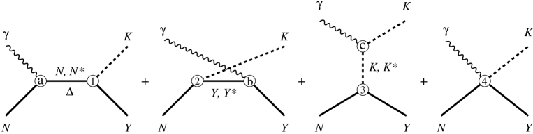
FIG. 1.: Feynman diagram for kaon photoproduction on the nucleon. Contributions from the $\Delta$ are only possible in $\Sigma$ production. Electromagnetic vertices are denoted by (a), (b), and (c), hadronic vertices by (1), (2), and (3). The contact diagram (4) is required in both PS and PV couplings in order to restore gauge invariance after introducing hadronic form factors. The Born terms contain the $N$, $Y$, $K$ intermediate states and the contact term.

FIG. 2.: Total cross sections for the six isospin channels of kaon photoproduction on the nucleon calculated at tree level. The solid curve shows Set II of Table III while the dotted line shows the older model, Set I of Table III. The new SAPHIR data [37] are denoted by the solid squares, old data [53] are shown by the open circles. Solid circles are the data for $K^{0}\Sigma^{+}$ production from Ref. [54].

FIG. 3.: Contribution of the Born terms (dashed lines), Born + $K^{*}$ + $K_{1}$ terms (dotted lines), and full operator (solid lines) to the total cross section of the $p(\gamma,K^{+})\Lambda$ and $p(\gamma,K^{+})\Sigma^{0}$ channels. The notation of the data is as in Fig. 2.

FIG. 4.: Differential cross section for $p(\gamma,K^{+})\Lambda$ channel. The notation of the curves is as in Fig. 2. The total c.m. energy $W$ is shown in every panel.

FIG. 5.: Differential cross section for $p(\gamma,K^{+})\Sigma^{0}$ channel. The notation of the curves is as in Fig. 2. The total c.m. energy $W$ is shown in every panel.

FIG. 6.: Differential cross section for $p(\gamma,K^{0})\Sigma^{+}$ channel. Data are from Ref. [54]. Notation is as in Fig. 2. The total c.m. energy $W$ is shown in every panel.

FIG. 7.: $\Lambda$ and $\Sigma$ recoil polarization for $p(\gamma,K^{+}){\vec{Y}}$. Notation is as in Fig. 2. The total c.m. energy $W$ is shown in every panel.

FIG. 8.: Target asymmetry for the reaction ${\vec{p}}(\gamma,K^{+})Y$. Notation is as in Fig. 2. The total c.m. energy $W$ is shown in every panel.

FIG. 9.: Photon asymmetry of $p({\vec{\gamma}},K^{+})Y$. Notation is as in Fig. 2. The total c.m. energy $W$ is shown in every panel.

FIG. 10.: Hyperon optical potentials for ¹²C at 300 MeV. The upper panels show the Dirac vector and scalar potentials, while the lower panels show the corresponding Schrödinger equivalent central and spin-orbit potentials. The three curves correspond to the $\Lambda$ (dashed), $\Sigma^{0}$ (dotted), and proton (solid) potentials.

FIG. 11.: Same as Fig. 10, showing the energy dependence at a fixed distance of $r=1$ fm.

FIG. 12.: Effects of final state interactions under quasifree kinematics for the reaction ${}^{12}{\rm C}(\gamma,KY)^{11}{\rm B}_{\rm g.s.}$ at $E_{\gamma}=1.4$ GeV and $p_{m}=120$ MeV. The four curves correspond to calculations in PWIA (dashed), in DWIA with only kaon FSI (dotted), with only hyperon FSI (dash-dotted), and the full DWIA(solid).

FIG. 13.: Total and individual contributions from the Born and resonance terms under the quasifree kinematics of Fig. 12. The three curves correspond to the full (solid), Born only (dotted), and resonance only (dashed) contributions of the elementary amplitude. The calculations were done in DWIA.

FIG. 14.: Same as Fig. 12, but under open kinematics, with $\theta_{K}=30^{\circ}$, $\theta_{Y}=35^{\circ}$, and $T_{K}=450$ MeV.

FIG. 15.: Effects of varying the scaling factors in the hyperon potentials under open kinematics. The solid line is in full DWIA ($\alpha_{v}\simeq\alpha_{s}\simeq 0.67$), the dotted line is with $\alpha_{v}=0.333$ and $\alpha_{s}=0.345$, and the dashed line is with $\alpha_{v}=\alpha_{s}=1$.

FIG. 16.: Effects of varying the $\Sigma N\rightarrow\Lambda N$ conversion factors in the hyperon potentials under open kinematics. The solid line displays the full DWIA calculation, the dotted line shows the result with the conversion potential turned off, and the dashed line is obtained by doubling the strength of the conversion potential.

FIG. 17.: Effects of turning on and off the real and imaginary parts of the hyperon potentials under open kinematics. The solid line is in full DWIA, the dotted line is with the imaginary part turned off, and the dashed line is with the real part turned off.