DPNU-99-23 KFKI-1999-03/A Back-to-Back Correlations for Bosons Modified by Medium

Abstract

Novel back-to-back correlations are shown to arise for thermal ensembles of squeezed bosonic states associated with medium-modified mass-shifts. The strength of these correlations could become unexpectedly large in heavy ion collisions.

1 INTRODUCTION

In this paper we consider the effect of possible mass shifts in the dense medium on two boson correlations in general. Thus far medium modifications of hadron masses have been mainly considered in terms of effects on such observables as dilepton yields and spectra. Hadron mass shifts are caused by interactions in a dense medium and therefore vanish on the freeze-out surface. Thus, a naive first expectation is that in medium hadron modifications may have little or no effect on two boson correlations, and so the usual Hanbury-Brown Twiss (HBT) effect [1] has been expected to be only concerned with the geometry and matter flow gradients on the freeze-out surface. However, in this paper we show that an interesting quantum mechanical correlation is induced due to the fact that medium modified bosons can be represented in terms of two-mode squeezed states of the asymptotic bosons, which are observables.

In this paper we assume the validity of relativistic hydrodynamics up to freeze-out. The local temperature $T(x)$ and chemical potential $\mu(x)$ are given. In relativistic heavy ion collisions at CERN SPS, it has been observed that the one particle spectra [2], simultaneously with the two particle correlation function, can be described by (local) thermal distributions fairly precisely [3]. We assume that the sudden approximation is a valid abstraction in describing the freeze-out process in relativistic heavy ion collisions quantum mechanically and that there exists an abrupt freeze-out surface, $\Sigma^{\mu}(x)$.

Let us consider the following model Hamiltonian for a scalar field $\phi({\bf x})$ in the rest frame of matter,

$${H}=H_{0}-\frac{1}{2}\int d{\bf x}d{\bf y}\phi({\bf x})\delta M^{2}({\bf x}-{\bf y})\phi({\bf y}),\quad H_{0}=\frac{1}{2}\int d{\bf x}\left(\dot{\phi}^{2}+|\nabla\phi|^{2}+m_{0}^{2}\phi^{2}\right),$$ (1)

where $H_{0}$ is the asymptotic Hamiltonian. The field $\phi({\bf x})$ in $H$ corresponds to quasi - particles that propagate with a momentum-dependent effective mass, which is related to the vacuum mass, $m_{0}$, via $m_{*}^{2}({|{\bf k}|})=m_{0}^{2}-\delta M^{2}({|{\bf k}|})$. The mass-shift is assumed to be limited to long wavelength collective modes.

The invariant single-particle and two-particle momentum distributions are given by

$$N_{1}({\bf k}_{1}) = \omega_{{\bf k}_{1}}{d^{3}N\over d{\bf k}_{1}}=\omega_{{\bf k}_{1}}\langle a^{\dagger}_{{\bf k}_{1}}a^{\phantom{\dagger}}_{{\bf k}_{1}}\rangle,$$ (2)

$$N_{2}({\bf k}_{1},{\bf k}_{2}) = \omega_{{\bf k}_{1}}\omega_{{\bf k}_{2}}\langle a^{\dagger}_{{\bf k}_{1}}a^{\dagger}_{{\bf k}_{2}}a^{\phantom{\dagger}}_{{\bf k}_{2}}a^{\phantom{\dagger}}_{{\bf k}_{1}}\rangle$$ (3)

$$= \omega_{{\bf k}_{1}}\omega_{{\bf k}_{2}}(\langle a^{\dagger}_{{\bf k}_{1}}a^{\phantom{\dagger}}_{{\bf k}_{1}}\rangle\langle a^{\dagger}_{{\bf k}_{2}}a^{\phantom{\dagger}}_{{\bf k}_{2}}\rangle+\langle a^{\dagger}_{{\bf k}_{1}}a^{\phantom{\dagger}}_{{\bf k}_{2}}\rangle\langle a^{\dagger}_{{\bf k}_{2}}a^{\phantom{\dagger}}_{{\bf k}_{1}}\rangle+\langle a^{\dagger}_{{\bf k}_{1}}a^{\dagger}_{{\bf k}_{2}}\rangle\langle a^{\phantom{\dagger}}_{{\bf k}_{2}}a^{\phantom{\dagger}}_{{\bf k}_{1}}\rangle),$$

where $a_{\bf k}$ is the annihilation operator for the asymptotic quantum with four-momentum $k^{\mu}\,=\,(\omega_{\bf k},{\bf k})$, $\omega_{\bf k}^{2}={m_{0}^{2}+{\bf k}^{2}}$ and the expectation value of an operator $\hat{O}$ is given by the density matrix $\hat{\rho}$ as $\langle\hat{O}\rangle={\rm Tr}\,\hat{\rho}\,\hat{O}$.

We introduce the chaotic and squeezed amplitudes, defined, respectively, as

$$G_{c}(1,2)=\sqrt{\omega_{{\bf k}_{1}}\omega_{{\bf k}_{2}}}\langle a^{\dagger}_{{\bf k}_{1}}a^{\phantom{\dagger}}_{{\bf k}_{2}}\rangle,\quad G_{s}(1,2)=\sqrt{\omega_{{\bf k}_{1}}\omega_{{\bf k}_{2}}}\langle a^{\phantom{\dagger}}_{{\bf k}_{1}}a^{\phantom{\dagger}}_{{\bf k}_{2}}\rangle.$$ (4)

In most situations, the chaotic amplitude, $G_{c}(1,2)\equiv G(1,2)$ is dominant, and carries the Bose-Einstein correlations, while the squeezed amplitude, $G_{s}(1,2)$ vanishes:

$$C_{2}({\bf k}_{1},{\bf k}_{2})={N_{2}({\bf k}_{1},{\bf k}_{2})\over N_{1}({\bf k}_{1})N_{1}({\bf k}_{2})}=1+{|G(1,2)|^{2}\over G(1,1)G(2,2)}.$$ (5)

The exact value of the intercept, $C_{2}({\bf k},{\bf k})=2$, is a characteristic signature of a chaotic Bose gas without dynamical 2-body correlations.

2 RESULTS FOR A HOMOGENEOUS SYSTEM

The terms neglected in (5) involving $G_{s}(1,2)$ become non-negligible when $\delta M^{2}(|{\bf k}|)\neq 0$. Given such a mass shift, the dispersion relation is modified to $\Omega_{\bf k}^{2}=\omega^{2}_{\bf k}-\delta M^{2}(|{\bf k}|)$, where $\Omega_{\bf k}$ is the frequency of the in-medium mode with momentum ${\bf k}$. The annihilation operator for the in-medium quasi-particle with momentum ${\bf k}$, $b_{\bf k}$, and that of the asymptotic field, $a_{\bf k}$, are related by a Bogoliubov transformation [4]:

$$a^{\phantom{\dagger}}_{{\bf k}_{1}}=U^{\dagger}b^{\phantom{\dagger}}_{{\bf k}_{1}}U=c^{\phantom{\dagger}}_{{\bf k}_{1}}b^{\phantom{\dagger}}_{{\bf k}_{1}}+s^{*\phantom{\dagger}}_{-{\bf k}_{1}}b^{\dagger}_{-{\bf k}_{1}}\equiv C^{\phantom{\dagger}}_{1}+S^{\dagger}_{-1},$$ (6)

where $c_{\bf k}=\cosh[r_{\bf k}]$, $s_{\bf k}=\sinh[r_{\bf k}]$, and $r_{\bf k}=\frac{1}{2}\log(\omega_{\bf k}/\Omega_{\bf k})$. As is well-known, the Bogoliubov transformation is equivalent to a squeezing operation, and so we call $r_{\bf k}$ the mode dependent squeezing parameter. While it is the $a$-quanta that are observed, it is the $b$-quanta that are thermalized in medium. Thus, we consider the thermal average for a globally thermalized gas of the $b$-quanta, that is homogeneous in volume $V$:

$$\hat{\rho}={\displaystyle\phantom{|}1\over Z}\exp\left(-\frac{1}{T}\frac{V}{(2\pi)^{3}}\int d{\bf k}\,\Omega_{\bf k}\,b^{\dagger}_{\bf k}b^{\phantom{\dagger}}_{\bf k}\right).$$ (7)

When this thermal average is applied,

$$N_{1}({\bf k}) \!\!\!=\!\!\! \frac{V}{(2\pi)^{3}}\,\omega_{\bf k}\,n_{1}({\bf k}),~{}~{}n_{1}({\bf k})=|c_{\bf k}^{\phantom{\dagger}}|^{2}n_{\bf k}^{\phantom{\dagger}}+|s_{-\bf k}|^{2}(n_{-\bf k}+1),~{}~{}n_{\bf k}=\frac{1}{\exp(\Omega_{\bf k}/T)-1},$$

$$G_{c}(1,2) \!\!\!=\!\!\! \sqrt{\omega_{{\bf k}_{1}}\omega_{{\bf k}_{2}}}\left[\langle C^{\dagger}_{1}C^{\phantom{\dagger}}_{2}\rangle+\langle S^{\phantom{\dagger}}_{-1}S^{\dagger}_{-2}\rangle\right],~{}G_{s}(1,2)=\sqrt{\omega_{{\bf k}_{1}}\omega_{{\bf k}_{2}}}\left[\langle S^{\dagger}_{-1}C^{\phantom{\dagger}}_{2}\rangle+\langle C^{\phantom{\dagger}}_{1}S^{\dagger}_{-2}\rangle\right]\!.$$ (8)

In the homogeneous case, the resulting two particle correlation function is unity except for the parallel and anti-parallel cases. The dynamical correlation due to the two mode squeezing associated with mass shifts is therefore back-to-back as first pointed out in [4]. The HBT correlation intercept remains 2 for identical momenta. Evaluating $C_{2}({\bf k},{\bf-k})$ for $T\simeq 140$ MeV, $|{\bf k}|=0$ – 500 MeV for $\phi$ mesons, as a function of $m^{*}_{\phi}$, one finds back-to-back correlations (BBC) as big as 100 – 1000 for reasonable values of $m^{*}_{\phi}$. Note, that these novel BBC-s are not bounded from above, $1<C_{2}({\bf k},{\bf-k})<\infty$. With increasing values of $|{\bf k}|$ these BBC-s increase indefinitely. The huge BBC of decaying medium is, however, reduced if the decay of the medium is not completely sudden. To describe a more gradual freeze-out, the probability distribution $F(t_{i})$ of the decay times $t_{i}$ is introduced. The time evolution of $a_{\bf k}(t)$ is $a_{\bf k}(t)=a_{\bf k}(t_{i})\exp[-i\omega_{\bf k}(t-t_{i})]$, which leads to

$$C_{2}({\bf k},{\bf-k})=1+{\displaystyle\phantom{|}{|c^{*}_{\bf k}s_{\bf k}^{\phantom{\dagger}}n_{\bf k}^{\phantom{\dagger}}+c^{*}_{-\bf k}s_{-\bf k}^{\phantom{\dagger}}(n_{-\bf k}^{\phantom{\dagger}}+1)|^{2}}\over\displaystyle\phantom{|}{n_{1}({\bf k})\,n_{1}({-\bf k})}}\left|\int dtF(t)\exp\left[-i(\omega_{\bf k}+\omega_{-{\bf k}})t\right]\right|^{2}.$$ (9)

For a typical exponential decay, $F(t)=\theta(t-t_{0})\Gamma\exp[-\Gamma(t-t_{0})]$ with $\delta t=\hbar/\Gamma=2$ fm/c, we show the BBC for the $\phi$ mesons in Fig. 1, which shows that the BBC survives the suppression with a strength as large as 2-3.

3 RESULTS FOR INHOMOGENEOUS SYSTEMS

Following Ref.[5], we divide the inhomogeneous fluid into cells labeled $i$. In each cell, it is assumed that the field can be expanded with creation and annihilation operators, and that $H_{i}$ is diagonalized by a local Bogoliubov transformation, that implies

$$G_{c}(1,2) = {\displaystyle\phantom{|}1\over(2\pi)^{3}}\int d^{4}\sigma_{\mu}(x)K_{12}^{\mu}e^{iq_{12}x}\left[|c_{1,2}|^{2}n_{1,2}+|s_{-1,-2}|^{2}(n_{-1,-2}+1)\right],$$ (10)

$$G_{s}(1,2) = {\displaystyle\phantom{|}1\over(2\pi)^{3}}\int d^{4}\sigma_{\mu}(x)K_{12}^{\mu}e^{i2K_{12}x}\left[s^{*}_{-1,2}c_{2,-1}n_{-1,2}+c_{1,-2}s^{*}_{-2,1}(n_{1,-2}+1)\right].$$ (11)

Here $d^{4}\sigma^{\mu}(x)=d^{3}\Sigma^{\mu}(x;\tau_{f})\,F(\tau_{f})d\tau_{f}$ is the product of the normal-oriented volume element depending parametrically on $\tau_{f}$ (the freeze-out hypersurface parameter) and the invariant distribution of that parameter $F(\tau_{f})$. The other variables are defined as follows:

$$n_{i,j}(x) = 1/\left[\exp[(K^{*\mu}_{i,j}(x)u_{\mu}(x)-\mu(x))/T(x)]-1\right],$$ (12)

$$r(i,j,x) = \frac{1}{2}\log\left[(K^{\mu}_{i,j}(x)u_{\mu}(x))/(K^{*\mu}_{i,j}(x)u_{\mu}(x))\right],$$ (13)

$$c_{i,j} = \cosh[r({i,j},x)],\quad s_{i,j}\,=\,\sinh[r({i,j},x)],$$ (14)

where $i,j=\pm 1,\pm 2$ and the mean and the relative momenta for the $a$($b$)-quanta are defined as $K^{(*)\mu}_{i,j}(x)=[k^{(*)\mu}_{i}(x)+k^{(*)\mu}_{j}(x)]/2$ and $q^{\mu}_{i,j}=k^{\mu}_{i}-k^{\mu}_{j},$ respectively. The local hydrodynamical flow field is denoted by $u^{\mu}(x)$. See ref.  [6] for further details. The correlation function in the presence of local squeezing is given by

$$C_{2}({\bf k}_{1},{\bf k}_{2})=1+{|G_{c}(1,2)|^{2}\over G_{c}(1,1)G_{c}(2,2)}+{|G_{s}(1,2)|^{2}\over G_{c}(1,1)G_{c}(2,2)}.$$ (15)

As the Bogoliubov transformation always mixes particles with anti-particles, the above expression holds only for the case where particles are equivalent to their anti-particles, e.g. the $\phi$ meson and $\pi^{0}$. However, the extension to the case where particles and their anti-particles are different is straightforward; correlations between particles and anti-particles such as $\pi^{+}$ and $\pi^{-}$, $K^{+}$ and $K^{-}$, and so forth, appear [6]. Fig. 2 illustrates the novel character of BBC for two identical bosons caused by medium mass-modifications, along with the familiar Bose-Einstein or HBT correlations on the diagonal of the $({\bf k}_{1},{\bf k}_{2})$ plane.

4 SUMMARY

The theory of particle correlations and spectra for bosons with in-medium mass-shifts predicts the existence of back-to-back correlations of $\phi\phi$, $K^{+}K^{-}$, $\pi^{0}\pi^{0}$ and $\pi^{+}\pi^{-}$ pairs that could be searched for at CERN SPS and upcoming RHIC BNL heavy ion experiments [7]. Surprisingly, such novel back-to-back correlations could be as large as the well-known HBT correlations, surviving large finite time suppression factors.

Figure 1: Dependence of the back-to-back correlations (BBC) on the medium modified $\phi$ meson mass, $m^{*}_{\phi}$, for $T=140$ MeV, $\mu=0$, and $\delta t=2$ fm/c, where solid, dashed and dotted line stands for $|{\bf k}|=0$, 300 and 500 MeV, respectively. The magnitude of the BBC is large in spite of the finite time suppression.

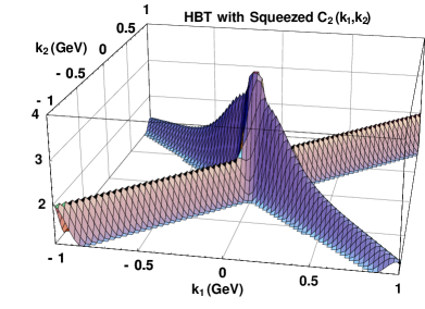
Figure 2: Schematic illustration of the new kind of correlations for mass shifted $\pi^{0}$ pairs, assuming $T=140$ MeV, $\delta t\!=\!0$ $G_{c}\!\sim\!\exp[-q_{12}^{2}R_{G}^{2}/2],G_{s}\!\sim\!\exp[-2K_{12}^{2}R_{G}^{2}]$, with $R_{G}\!=\!2$ fm. The fall of the BBC for increasing values of $|{\bf k}|$ is controlled here by a momentum-dependent mass-shift, $m^{*}_{\pi}\!=\!m_{\pi}[1+\exp(-{\bf k}^{2}/\Lambda_{s}^{2})]$ with $\Lambda_{s}=325$ MeV.

References

• [1] R. Hanbury-Brown and R.Q. Twiss, Phil.Mag. 45 (1954) 663.
• [2] I. G. Bearden et al., Phys. Rev. Lett. 78 (1997) 2080.
• [3] A. Ster, T. Csörgő, and B. Lörstad, in Proc. Quark Matter 99, Nucl. Phys. A (1999)
• [4] M. Asakawa and T. Csörgő, hep-ph/9612331, Heavy Ion Physics 4 (1996) 233.
• [5] A. Makhlin and Yu. Sinyukov, Sov. J. Nucl. Phys. 46 (1987) 354.
• [6] M. Asakawa, T. Csörgő, and M. Gyulassy, nucl-th/9810034.
• [7] W. A. Zajc and B. Lörstad, private communication.