FT-194-1980, August

Abstract

The original preprint was never published, due to various circumstances beyond the author’s control. The initial preprint has been known to a number of people, the results have been used in published literature and the preprint is still been referred to. The present text has been edited somewhat and a number of typos have been corrected; however, no significant changes have been incorporated into the text. No formulas have been added or deleted and the figures have been redrawn. A scanned copy of the original preprint in jpeg format can be found at
$http://www.phys.washington.edu/~{}bulgac/publications.html$

The author thanks F.M. Edwards for helping to edit the text and Yongle Yu for bringing to his attention a number of typos.

Some general features of the spectrum of the Hartree–Fock–Bogoliubov equations are examined. Special attention is paid to the asymptotic behavior of the single quasiparticle wave functions (s.qp.w.fs.), matter density distribution and density of the pair condensate. It is shown that due to the coupling between hole and particle states,the deeply bound hole states acquire a width and have to be treated as continuum states. The proper normalization of the s.qp.w.fs. is discussed.

I Introduction

The Hartree–Fock–Bogoliubov (HFB) approximation was outlined more than twenty years ago [1] for infinite systems and almost immediately was introduced in nuclear physics [2]. In the case of infinite systems the HFB procedure is well studied and the character of the wave–functions (w.f.) is well understood. However, in the case of finite systems (nuclei), things are not so clear. The HFB equations in the case of nuclei are meaningful provided the boundary conditions for the single quasiparticle (s.qp.) w.fs. are correctly formulated in order to describe a genuine finite state. The goal of the present paper is to provide the correct formulation of the HFB approximation in the case of finite systems.

It is well known that pairing correlations always appear whenever a pole (i.e. a bound state) is present in the two-body Green function of the many-body system [3]. In this case, corrections to the single particle (s.p.) Green function of the type

give rise to diagrams of the type

when only the contribution of the pole is taken into account [3]. Here $2\lambda$ stands for the energy of the two–particle bound state and $\varepsilon_{p}$ and $\varepsilon_{h}$ are the particle and hole energies respectively. The process represented by diagram (1) leads to a mixing between particle and hole states and as a result to a smearing of the Fermi surface [3, 4, 5]. This mixing has the special feature that a hole (particle) can transform into a particle (hole), due to the presence of the pair condensate, provided their energies are related by the energy conservation law

$\displaystyle\varepsilon_{p}+\varepsilon_{h}=2\lambda.$

Whenever the energy of the hole state is less than $2\lambda$ the corresponding particle state to which the hole state is coupled lies in continuum. This situation formally resembles the case of an electron in a very strong field [6] or the case of a bound state embedded in continuum [7]. Consequently, a sufficiently deep hole state becomes unstable with respect to decay into a particle state by an interaction with the pair condensate. The same thing happens in the case of a deep hole decaying into a less deeply bound hole, with the excitation of a phonon, which can further decay by particle emission. This process is described by the diagram

where the wavy line represents a phonon.

The physical situation is thus not new. New is the fact that due to the presence of the pair condensate, some hole states acquire a width and therefore the s.qp.w.fs. can no longer be treated as corresponding to bound states, as has hitherto been done, but as continuum states. How to introduce this property of the s.qp.w.fs. into the HFB approximation for finite systems and therefore how to define the boundary conditions correctly is the main goal of the present discussion.

II HFB equations for finite systems

In this section the well–known HFB equations will be derived for the sake of completeness. The emphasis will be on the correct definition of s.qp.w.fs. so as to describe genuine finite systems, i.e. systems with finite matter distribution. The forces between particles will not be specified, except for some general properties, like the finite range.

By analogy with the usual HF approximation, the HFB ground state w.f. $\mid 0\rangle$ is defined as the vacuum for the fermi quasiparticles [1, 2, 4, 5]

$$\alpha_{i}\mid 0\rangle=0\;\;,\quad\langle 0\mid 0\rangle=1,$$ (1)

where

$$\alpha_{i} = \int dx[u_{i}^{*}(x)_{i}\psi(x)+v_{i}(x)\psi^{\dagger}(x)],$$ (3)

$$\alpha_{i}^{\dagger} = \int dx[v_{i}^{*}(x)\psi(x)+u_{i}(x)\psi^{\dagger}(x)],$$ (4)

and $\psi(x)$ and $\psi^{\dagger}(x)$ stand for field operators for annihilation and creation of a particle with space–spin coordinates $x=(\vec{r},\sigma)$, which satisfy the usual anticommutation relations

$$\{\psi(x),\psi^{\dagger}(y)\}=\delta(x-y),$$ (5)

$$\{\psi(x),\psi(y)\}=(\psi^{\dagger}(x),\psi^{\dagger}(y))=0.$$ (6)

By requiring that $\alpha_{i}$ and $\alpha^{\dagger}_{i}$ represent fermion operators, i.e.

$$\{\alpha_{i},\alpha^{\dagger}_{j}\}=\delta_{ij},$$ (7)

$$\{\alpha_{i},\alpha_{j}\}=\{\alpha^{\dagger}_{i},\alpha^{\dagger}_{j}\}=0,$$ (8)

one easily obtains the relations

$$\int[u_{i}^{*}(x)u_{j}(x)+v_{i}(x)v_{j}^{*}(x)]dx=\delta_{ij},$$ (9)

$$\int[u_{i}^{*}(x)v_{j}(x)+v_{i}(x)u_{j}^{*}(x)]dx=0,$$ (10)

$$\sum_{i}u_{i}(x)u_{i}^{*}(y)+v_{i}(x)v_{i}^{*}(y)=\delta(x-y),$$ (11)

$$\sum_{i}u_{i}(x)v_{i}(y)+v_{i}(x)u_{i}(y)=0.$$ (12)

The constraints (5–6) ensure the unitary character of the transformations (3).

The total energy of the many–body system and the mean number of particles are

$\displaystyle{\cal E}=\langle 0\mid\hat{H}\mid 0\rangle$

and

$\displaystyle N=\langle 0\mid\hat{N}\mid 0\rangle,$

where $\hat{H}$ and $\hat{N}=\int dx\psi^{\dagger}(x)\psi(x)$ stand for the hamiltonian and the number operator in the second quantization representation.

The mean values for the energy and for the particle number can be expressed through the densities

$$\rho(x,y)=\langle 0\mid\psi^{+}(y)\psi(x)\mid 0\rangle=\rho^{*}(y,x)=\sum_{i}v_{i}(x)v_{i}^{*}(y),$$ (13)

$$\Phi(x,y)=\langle 0\mid\psi(y)\psi(x)\mid 0\rangle=-\Phi(y,x)=\sum_{i}v_{i}(x)u_{i}(y),$$ (14)

in the following way

$${\cal E}={\rm Tr}(T\rho)+\frac{1}{2}{\rm Tr}(V\rho\rho)_{a}+\frac{1}{2}{\rm Tr}(V\Phi\Phi^{*}),$$ (15)

$${\rm N}={\rm Tr}(\rho),$$ (16)

if only two–body interactions are present. $T$ and $V$ stand for the kinetic energy and the two–body interaction respectively. A shorthand notation was used for the traces in Rels. (9) and (10).

The HFB equations for the two component s.qp.w.fs. $\{v_{i}(x),u_{i}^{*}(x)\}$ are derived from the stationarity condition of the total energy (9) under the subsidiary conditions (10) and (5). These equations are

$$\int h(x,y)v_{i}(y)dy-\lambda v_{i}(x)+\int\Delta(x,y)u_{i}^{*}(y)dy=E_{i}v_{i}(x)$$ (17)

$$\int\Delta^{\dagger}(x,y)v_{i}(y)dy-\int h^{*}(x,y)u_{i}^{*}(y)dy+\lambda u_{i}^{*}(x)=E_{i}u_{i}(x)$$ (18)

where

$\displaystyle\lambda=\frac{\delta{\cal E}}{\delta N}<0$

is the chemical potential, and

$\displaystyle h(x,y)=\frac{\delta{\cal E}}{\delta\rho(x,y)}=h^{*}(y,x)$

and

$\displaystyle\Delta(x,y)=\frac{\delta{\cal E}}{\delta\Phi^{*}(x,y)}=-\Delta(y,x)$

are the s.p. hamiltonian and the pairing field respectively and $E_{i}$ stands for the s.qp. energies.

When performing the summations in Rels. (7) and (8) one must include only those solutions of the nonlinear system (11–12) with $E_{i}<0$, which define the operators $\alpha_{i}^{\dagger}$. The solutions with $E_{i}>0$ correspond to operators $\alpha^{\dagger}_{i}$.

Let us analyse in more detail these equations in the case of a finite system. The problem which arises is the meaning of the normalization condition (5); namely, if the right hand side of Rel. (5) should be a $\delta$–function or a Kronecker symbol, as is usually the case [2, 5, 8, 9], in complete analogy with the HF approximation.

A finite system is characterized by a finite matter distribution and therefore by a finite range of the s.p. field (except in the case of the Coulomb interaction). Naturally, being determined by the matter distribution, the pairing field must also have a finite range (an infinite range of the pairing field can only occur if the system under consideration is unstable with respect to two particle decay.) The problem is determining the mechanism which leads to finite matter distribution when s.qp. states no longer have the character of discrete states, as was discussed in the Introduction.

When pairing is turned off (i.e. $\Delta\equiv 0$) the spectrum of Eqs. (11–12) looks like the one show in Fig. 1. The left hand side corresponds to the spectrum of Eq. (11), while the right hand side corresponds to Eq. (12).

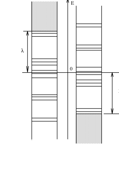
FIG. 1.: The spectra of Eqs. (11–12) when the pairing field is turned off ($\Delta=\equiv 0$). The left hand side corresponds to the spectrum of Eq. (11), while the right hand side corresponds to Eq. (12) . The hatched regions represent the continuum and the lines correspond to discrete states.

Upon turning the pairing on, the two spectra mix and the discrete states with energies outside the interval

$$\lambda<E<-\lambda$$ (19)

will lie in the continuum. Only the states with energy within the interval (13) will preserve the bound state character.

The continuum part of the spectrum for $E<\lambda$ and $E>-\lambda$ can disappear only if the s.p. potential is finite and positive at infinity as in the case of a harmonic oscillator. There is no physical reason for this to be true in the case of finite systems.

A glance at Fig.1. reveals why pairing correlations lead to a significant increase of the level density in the vicinity of the Fermi surface. Pairing appears when the chemical potential has a value within a shell, as illustrated in Fig. 1. In such a case, the total number of hole (the left hand side of Fig. 1) and particle (the right hand side of Fig. 1) states, which is practically equal to the number of s.qp. states with pairing included, is almost double the number of s.p. states in HF approximation.

In order to determine what happens in the case of a bound state with an energy $E$, when pairing is turned on, we shall use perturbation theory. For the sake of simplicity, the nucleus will be assumed to be spherical and the pairing field real $\Delta\equiv\Delta^{*}$. Also, the spin and angular variables are assumed to be already separated from Eqs. (11) and (12) and the corresponding geometrical factors included in the definition of the single particle fields. From Eq. (11) one easily obtains in the vicinity of a bound state the relation

$$v_{E}(r)=\left(\frac{1}{E+\lambda-h}\Delta u_{E}\right)(r)\cong\phi_{0}(r)\frac{\langle\phi_{0}\mid\Delta\mid u_{E}\rangle}{E-E_{0}}=n^{1/2}(E)\phi_{0}(r),$$ (20)

where

$\displaystyle(h-\lambda-E_{0})\phi_{0}=0\;\;,\;\;\langle\phi_{0}\mid\phi_{0}\rangle=1.$

The other component of the single quasi–particle wave function becomes then

$$u_{E}(r)=C(E)u_{0E}(r)-n^{1/2}(E)\left(\frac{1}{-E+\lambda-h}\Delta\phi_{0}\right)(r),$$ (21)

where

$$(h-\lambda+E)u_{0E}=0,\quad\langle u_{0E}\mid u_{0E^{\prime}}\rangle=\delta(E-E^{\prime})$$ (22)

and $C(E)$ is a normalization constant. From Rels. (14) and (15) one obtains

$\displaystyle n^{1/2}(E)=\frac{C(E)\langle\phi_{0}\mid\Delta\mid u_{0E}\rangle}{E-E_{0}+\langle\phi_{0}\mid\Delta\frac{1}{-E+\lambda-h}\Delta\mid\phi_{0}\rangle}.$

In order to determine the normalization constant $C(E)$, we shall use the representation of the Green function through regular and irregular solutions of Eq. (16)

$\displaystyle G(r,r^{\prime},-E+\lambda)=\left(\frac{1}{-E+\lambda-h}\right)(r,r^{\prime})=\frac{2m}{\hbar^{2}}\frac{u_{0E}(r_{<})\chi_{E}(r_{>})}{W(u_{0E},\chi_{E})}$

where $W(u_{0E},\chi_{E})$ stands for the Wronskian

$\displaystyle W(u_{0E},\chi_{E})=-\frac{2m}{\pi\hbar^{2}}.$

The asymptotic behavior for the regular $u_{0E}$ and irregular $\chi_{E}$ solutions is given by

$$u_{0E}(r)\cong\sqrt{\frac{2m}{\hbar^{2}\pi k}}\sin(kr+\delta_{0E}),$$ (23)

$$\chi_{E}(r)\cong\sqrt{\frac{2m}{\hbar^{2}\pi k}}\cos(kr+\delta_{0E}),$$ (24)

where $k^{2}=2m(-E+\lambda)/\hbar^{2}$. The asymptotic behavior of the $u$–component is

$\displaystyle u_{E}(r)\cong\sqrt{\frac{2m}{\hbar^{2}\pi k}}[C(E)\sin(kr+\delta_{0E})+\pi n^{1/2}(E)\langle\phi_{0}\mid\Delta\mid u_{0E}\rangle\cos(kr+\delta_{0E})],$

and therefore

$$C^{2}(E)=\frac{[E-E_{0}+\langle\phi_{0}\mid\Delta\frac{1}{-E+\lambda-h}\Delta\mid\phi_{0}\rangle]^{2}}{[E-E_{0}+<\phi_{0}\mid\Delta\frac{1}{-E+\lambda-h}\Delta\mid\phi_{0}>]^{2}+\pi^{2}\mid<\phi_{0}\mid\Delta\mid u_{0E}>\mid^{4}}.$$ (25)

Consequently, the normalized solutions are

$$v_{E}(r)=n^{1/2}(E)\phi_{0}(r)$$ (26)

$$u_{E}(r)=C(E)u_{0E}(r)-n^{1/2}(E)\left(\frac{1}{-E+\lambda-h}\Delta\phi_{0}\right)(r)\;,$$ (27)

where

$$n(E) = \frac{1}{\pi}\quad\frac{\frac{1}{2}\Gamma(E)}{(E-E_{0}-\delta E)^{2}+\frac{1}{4}\Gamma^{2}(E)}\;,$$ (28)

$$\Gamma(E) = 2\pi|\langle\phi_{0}\mid\Delta\mid u_{0E}\rangle|^{2}=2\pi\frac{\mid\langle\phi_{0}\mid[h,\Delta]\mid u_{0E}\rangle\mid^{2}}{(E+E_{0})^{2}},$$ (29)

$$\delta E = -\langle\phi_{0}\mid\Delta\frac{1}{-E+\lambda-h}\Delta\mid\phi_{0}\rangle$$ (30)

and

$$\int_{\infty}^{\infty}n(E)dE=1.$$ (31)

The matrix elements in the above relations can be calculated without any significant loss of accuracy for $E=E_{0}$.

As one can observe, due to the coupling with the continuum, the bound state spreads over the entire spectrum (see Rel. (21)). Now the quantity $n(E)$ has thus to be interpreted as the occupation number probability density over a unit energy interval.

The solution is formally equivalent to the solution of a coupled channel problem with a bound state embedded in the continuum[7]. It displays a well–defined resonant character with a width $\Gamma(E_{0})$ and a shift $\delta E$. The case of a resonant state can be treated in a similar way.

Far from the resonance energy $E_{0}$, the amplitude of the $u$–component is very small, while the $u$–component is practically equal to the unperturbed solution $u_{0E}$. In the vicinity of the resonance $E_{0}$, the amplitude of the $u$–component increases significantly inside the potential well (see Rels. (18), (20)), while the phase of the $u$–component changes by $\pi$. The phase of the $u$–component is

$\displaystyle\delta_{E}=\delta_{0E}-\arctan\frac{\Gamma(E)}{2(E-E_{0}-\delta E)}$

The solution just described is characterized by the fact that the $v$–component is square integrable, even though the single quasi–particle wave function solution $(v_{E}(x),u^{*}_{E}(x))$ represents a continuum state. The question is: does this feature hold true for the selfconsistent solution of the HFB equations?

The density distribution $\rho$ satisfies Rel. (10) (i.e. the diagonal part of $\rho$ is integrable), while the density of the pair condensate satisfies the condition

$$\int\mid\Phi(x,y)\mid^{2}=Tr[\rho(1-\rho)]<N,$$ (32)

which can be easily derived by means of Rels. (5–6) [1, 4, 5, 8]. Therefore, one can expect that $\rho$ and $\Phi$ both fall down quickly enough outside the system. The density distribution $\rho$ determines the asymptotic behavior of the single particle selfconsistent potential $U$, while the density $\Phi$ defines the pairing potential $\Delta=V\Phi/2$.

The nonlocality of these potentials is governed by the range of the two–body interaction $V$, assumed to be finite.

We shall now show that the following asymptotic behaviors take place

$$U\sim\rho\sim{\cal{O}}\left(\exp\left[2\sqrt{\frac{2m\mid\lambda\mid}{\hbar^{2}}}r\right]\right)$$ (33)

and

$$\Delta\sim\Phi\sim{\cal{O}}\left(\exp\left[\sqrt{2\frac{2m\mid\lambda\mid}{\hbar^{2}}}r\right]\right),$$ (34)

when $\mathchoice{{\hbox{\boldmath$\displaystyle R$}}}{{\hbox{\boldmath$\textstyle R$}}}{{\hbox{\boldmath$\scriptstyle R$}}}{{\hbox{\boldmath$\scriptscriptstyle R$}}}=(\mathchoice{{\hbox{\boldmath$\displaystyle r$}}}{{\hbox{\boldmath$\textstyle r$}}}{{\hbox{\boldmath$\scriptstyle r$}}}{{\hbox{\boldmath$\scriptscriptstyle r$}}}+\mathchoice{{\hbox{\boldmath$\displaystyle r$}}}{{\hbox{\boldmath$\textstyle r$}}}{{\hbox{\boldmath$\scriptstyle r$}}}{{\hbox{\boldmath$\scriptscriptstyle r$}}}^{\prime})/2$ tends to infinity and $\mathchoice{{\hbox{\boldmath$\displaystyle s$}}}{{\hbox{\boldmath$\textstyle s$}}}{{\hbox{\boldmath$\scriptstyle s$}}}{{\hbox{\boldmath$\scriptscriptstyle s$}}}=\mathchoice{{\hbox{\boldmath$\displaystyle r$}}}{{\hbox{\boldmath$\textstyle r$}}}{{\hbox{\boldmath$\scriptstyle r$}}}{{\hbox{\boldmath$\scriptscriptstyle r$}}}-\mathchoice{{\hbox{\boldmath$\displaystyle r$}}}{{\hbox{\boldmath$\textstyle r$}}}{{\hbox{\boldmath$\scriptstyle r$}}}{{\hbox{\boldmath$\scriptscriptstyle r$}}}^{\prime}$ remains finite (practically of the order of the range of $V$). (In the above Rels. (23–24) the symbol ${\cal{O}}$ means that the quantities on the left hand side behave like the corresponding arguments of the ${\cal{O}}$–function.) As one can observe, the pairing field $\Delta$ has a longer tail than the s.p. selfconsistent field $U$.

Using Rels. (23) and (24) one can show, using HFB Eqs. (11–12), that the $v$– and $u$–components behave asymptotically as

$$v(r)\sim\exp\left(-\sqrt{\frac{2m}{\hbar^{2}}\mid E+\lambda\mid}r\right),$$ (35)

$$u(r)\sim\exp\left(-\sqrt{\frac{2m}{\hbar^{2}}\mid E-\lambda\mid}r\right),$$ (36)

if

$$\lambda<E<0,$$ (37)

and

$$v(r)\sim\exp\left(-\sqrt{\frac{2m}{\hbar^{2}}\mid 2\lambda\mid}r\right),$$ (38)

$$u(r)\sim{\cal{O}}(1),$$ (39)

if

$$E<\lambda.$$ (40)

Outside the potential well, for energies in the interval (27), the two Eqs. (11–12) decouple and the corresponding asymptotic behavior of the $v$– and $u$–components of the single quasi–particle wave function is determined by the “energies” $\lambda+E$ and $\lambda-E$, respectively. For energies in the interval (30,) the asymptotic behavior of the $v$–component is governed by the inhomogeneous part of the Eq. (11) (i.e. by the term $\Delta u^{*}$), which cannot be neglected in this case, as was possible for energies in the interval (27). On the other hand, the term $\Delta^{\dagger}v$ falls down exponentially and does not influence the asymptotic behavior of the $u$–component.

The asymptotic behavior of the $u$–component is fully determined by the “energy” $-E+\lambda$, which is positive in the interval (30).

Now, if one takes into account the definitions of densities $\rho$ and $\Phi$ (Rels. (7) and (8) respectively), one can easily notice that the asymptotic behavior of the $v$– and $u$–components (see Rels. (25–30)) completely agrees with the asymptotic behaviors (23) and (24). This means that the corresponding asymptotic behaviors are selfconsistent. It is physically natural to expect that the asymptotic behavior of the density $\rho$ is controlled by the chemical potential $\lambda$, i.e. by the energy of the least bound particle. The density of the pair condensate $\Phi$ can be interpreted as the wave function of a bound state of two interacting particles in an external field with energy $2\lambda$. Using HFB Eqs. (11) and (12) and the definition (8), one can show that the density $\Phi$ satisfies the equation [1]

$$(h(1)+h(2)+v(1,2)-2\lambda)\Phi(1,2)=$$ (41)

other terms negligible outside the system .

From this equation it follows that at large distances $\Phi$ behaves as

$\displaystyle\exp\left(-\alpha r_{1}-\beta r_{2}\right),$

where

$\displaystyle-(\alpha^{2}+\beta^{2})=\frac{2m}{\hbar^{2}}2\lambda,$

which also agrees with Rel. (24).

Strictly speaking, this asymptote is correct only outside the range of $V$. If,however, one takes into account the fact that a system of two identical nucleons does not have bound states, the asymptote is valid everywhere outside the s.p. potential well.

Summing up, in the normalization conditions (5) for the single quasi-particle wave functions, the right hand side has to be interpreted as a Kronecker symbol if $\lambda<E<-\lambda$ and as a Dirac $\delta$–function if $\mid E\mid>\mid\lambda\mid$ (as it is well known [1, 2, 3, 4, 5, 8] the system (11–12) has the property that if $\{v_{i},u^{*}_{i},E_{i}\}$ is a solution, then $\{u_{i},v^{*}_{i},-E_{i}\}$ is a solution as well). Furthermore, for $E<0$ the $v$–component of the single quasi–particle wave function is always square integrable and its norm has to be interpreted as the occupation number probability. On the other hand, the relation

$\displaystyle 1-n_{i}=1-\int\mid v_{i}(x)\mid^{2}dx=\int\mid u_{i}(x)\mid^{2}dx$

is valid only for $\lambda<E<-\lambda$. If the energy $E$ is outside this interval, the integral $\int|v_{i}(x)|^{2}dx$ should be interpreted as an occupation number probability density per unit energy interval.

III Some simple examples

This section is devoted to some simple examples of HFB equations, which although somewhat unrealistic, lead to a better understanding of various issues arising while solving Eqs. (11–12).

A Constant pairing approximation $\Delta\equiv$ constant

This approximation is also known as the BCS approximation [10]. The s.qp.w.f. in this case is

$$v(r) = n^{1/2}_{BCS}\phi(r),$$ (42)

$$u(r) = \sqrt{1-n_{BCS}}\phi(r),$$ (43)

where

$$(h-\epsilon)\phi=0,\quad n_{BCS}=\frac{1}{2}\left(1-\frac{\epsilon-\lambda}{\sqrt{\epsilon-\lambda)^{2}+\Delta^{2}}}\right)$$ (44)

and

$\displaystyle E=-\sqrt{(\epsilon-\lambda)^{2}+\Delta^{2}}.$

Usually, the pairing field $\Delta\equiv$ const is taken to be different from zero in a limited energy interval around the Fermi surface. However, there is no recipe to determine this energy band in a unique way. It is obvious that the density $\rho$ cannot be integrable if solutions belonging to the continuum part of the spectrum of the Eq. (32) are included (i.e. when the pairing field is nonvanishing for such states). Furthermore, if one considers that $\Delta$ is acting for all energies, then the density $\Phi$ is

$$\Phi(x,y) = \sum_{i}\phi_{i}(x)\phi^{*}_{i}(y)\frac{\Delta}{2\sqrt{(\varepsilon_{i}-\lambda)^{2}+\Delta^{2}}},$$ (45)

$$= \frac{\Delta}{2}\sum_{i}\phi_{i}(x)\phi^{*}_{i}(y)\left[\frac{1}{\sqrt{(\varepsilon_{i}-\lambda)^{2}+\Delta^{2}}}-\frac{1}{\varepsilon_{i}-\lambda}\right]-\frac{\Delta}{2}G(x,y,\lambda),$$ (46)

where $G(x,y,\lambda)$ stands for the single particle Green function of the Eq. (32). As is well known, the Green function diverges like $\mid\mathchoice{{\hbox{\boldmath$\displaystyle r$}}}{{\hbox{\boldmath$\textstyle r$}}}{{\hbox{\boldmath$\scriptstyle r$}}}{{\hbox{\boldmath$\scriptscriptstyle r$}}}-\mathchoice{{\hbox{\boldmath$\displaystyle r$}}}{{\hbox{\boldmath$\textstyle r$}}}{{\hbox{\boldmath$\scriptstyle r$}}}{{\hbox{\boldmath$\scriptscriptstyle r$}}}^{\prime}\mid^{-1}$ when $\mathchoice{{\hbox{\boldmath$\displaystyle r$}}}{{\hbox{\boldmath$\textstyle r$}}}{{\hbox{\boldmath$\scriptstyle r$}}}{{\hbox{\boldmath$\scriptscriptstyle r$}}}\rightarrow\mathchoice{{\hbox{\boldmath$\displaystyle r$}}}{{\hbox{\boldmath$\textstyle r$}}}{{\hbox{\boldmath$\scriptstyle r$}}}{{\hbox{\boldmath$\scriptscriptstyle r$}}}^{\prime}$. Therefore, a finite density $\Phi$ cannot be defined in this case because of this divergence. One notices that the divergence is not logarithmic, as is usually stated in textbooks [3, 10]. A local pairing field corresponds to a zero range two–body interaction. Then, as one can easily show by using Eq. (31), the density $\Phi$ will always be singular for coinciding arguments. For the entire HFB procedure to be meaningful, the two–body interaction, which is responsible for pairing, must have a finite range.

B Square well single particle potential and square well pairing potential

We assume that

$$U(r) = U_{0}\theta(R-r),\quad U_{0}<0,$$ (47)

$$\Delta(r) = \Delta_{0}\theta(R-r),$$ (48)

and look for solutions of Eqs. (11–12) with zero orbital momentum $l=0$.

For $r<R$ the solution reads

$$v_{in}(r) = C_{+}\sin k_{+}r+C_{-}\sin k_{-}r,$$ (49)

$$u_{in}(r) = \beta_{+}C_{+}\sin k_{+}r+\beta_{-}C_{-}\sin k_{-}r,$$ (50)

where

$$\beta_{\pm}=\frac{E\mp\sqrt{E^{2}-\Delta^{2}_{0}}}{\Delta_{0}},\quad\beta_{+}\beta_{-}=1$$ (51)

and $C_{\pm}$ stand for some constants, which have to be determined from matching the interior with the exterior solutions and normalization.

For $r>R$

$$v_{out}(r)=v_{0}\exp(-k_{0}r),\quad{\rm if}\quad\frac{\hbar^{2}}{2m}k^{2}_{0}=-(E+\lambda)>0,$$ (52)

$$u_{out}(r)=u_{0}\exp(-ik_{0}^{\prime}r)\quad{\rm if}\quad\frac{\hbar^{2}}{2m}k^{\prime 2}_{0}=-(-E+\lambda)>0$$ (53)

or

$\displaystyle u_{out}(r)=u_{1}\sin k^{\prime}_{0}r+u_{2}\cos k^{\prime}_{0}r$

if

$\displaystyle\frac{\hbar^{2}}{2m}k^{\prime 2}_{0}=-E+\lambda>0$

where $v_{0},u_{0},u_{1}$ and $u_{2}$ have to be determined from matching and normalization.

If $\lambda<E<-\lambda$, the spectrum is discrete and the energies have to be determined from the matching condition

$\displaystyle\frac{\beta_{+}(k_{-}\cos k_{-}R+k_{0}\sin k_{-}R)(k_{+}\cos k_{+}R+k^{\prime}_{0}\sin k_{+}R)}{\beta_{-}(k_{-}\cos k_{-}R+k^{\prime}_{0}\sin k_{-}R)(k_{+}\cos k_{+}R+k_{0}\sin k_{+}R)}=1.$

If $E<\lambda$ , then one deals with a state lying in continuum. In contrast to the case of constant pairing, one now has $[h,\Delta]\neq 0$ and sufficiently deeply bound hole states acquire width.

Inside the potential well, the two components of the s.qp.w.f. form a superposition of two s.p.w.f. with energies equal approximately to $E+\lambda+U_{0}$ and $-E+\lambda+U_{0}$, respectively (as a rule $\Delta_{0}$ is very small and can be neglected in the determination of $k_{\pm}$).

In the vicinity of a hole state (the left hand side of Fig. 1) $C_{+}$ has a zero and one can show that

$\displaystyle\frac{v_{in}(r)}{u_{in}(r)}\cong\beta_{+}\cong\frac{2E}{\Delta_{0}}\cong\sqrt{\frac{n_{BCS}}{1-n_{BCS}}},\quad n_{BCS}\cong 1,$

similar to the BCS approximation. This relation holds only inside the potential well and it is not valid outside it. Far from the resonance this ratio becomes

$\displaystyle\frac{u_{in}(r)}{v_{in}(r)}\cong\beta_{+}\cong\frac{2E}{\Delta_{0}}\cong\sqrt{\frac{1-n_{BCS}}{n_{BCS}}},\quad n_{BCS}\ll 1.$

Unlike the BCS approximation, the radial behaviors of the $v$– and $u$–components are no longer identical.

In this case, the density $\rho$ has the correct asymptotic behavior, but due to the local character of the pairing potential, the density $\Phi$ has the same divergence as in the case of BCS approximation. .

C Surface pairing $\Delta=\Delta_{0}\delta(r-R)$

This is another approximation which has been used in nuclear physics. The solution of Eqs. (11–12) is now

$$v(r)=\Delta_{0}G(r,R,E+\lambda)u(R),$$ (54)

$$u(r)=\kappa u_{0}(r)-\Delta^{2}_{0}G(r,R,-E+\lambda)G(R,R,E+\lambda)u(R),$$ (55)

where

$\displaystyle u(r)=\frac{\kappa u_{0}(R)}{1+\Delta^{2}_{0}G(R,R,-E+\lambda)G(R,R,E+\lambda)},$

$\kappa$ is a normalization constant and $u_{0}$ is given by the equation

$\displaystyle(h-\lambda+E)u_{0}=0$

($u_{0}$ has to be included only for $E<\lambda$)

The density $\rho$ has a correct asymptotic behavior, but the same problems arise with the density $\Phi$ as above. The density of the pair condensate $\Phi$ is singular for $\mathchoice{{\hbox{\boldmath$\displaystyle r$}}}{{\hbox{\boldmath$\textstyle r$}}}{{\hbox{\boldmath$\scriptstyle r$}}}{{\hbox{\boldmath$\scriptscriptstyle r$}}}=\mathchoice{{\hbox{\boldmath$\displaystyle r$}}}{{\hbox{\boldmath$\textstyle r$}}}{{\hbox{\boldmath$\scriptstyle r$}}}{{\hbox{\boldmath$\scriptscriptstyle r$}}}^{\prime}$ (see Eq. (31)).

Even though the examples discussed here have little in common with the real selfconsistent solution of Eqs. (11–12), in our opinion however, they lead to a deeper understanding of the structure of the HFB equations in the case of finite systems. Especially instructive in this sense is the role played by the nonlocality of the pairing field and consequently by the range of the two–body forces.

IV Conclusion

We have examined the HFB approximation in the case of finite systems, when the two–body interaction between particles has a finite range. Special attention was paid to the asymptotic behavior of the s.qp.w.fs. It was shown that the s.qp. states located in spectrum sufficiently far from the Fermi surface have the character of continuum states. E.g. the deep hole states acquire a width corresponding to the decay into a particle state and the pair condensate. This width has to be interpreted as a contribution to the imaginary part of the s.p. optical potential.

Even though most of the s.qp.w.fs. lie in continuum, the matter distribution is nevertheless finite. The same holds true for the density of the pair condensate, which is finite as well.

These features of the general solutions of the HFB equations have to be included in any HFB calculations. To what extent the available HFB results [8, 9] correspond to the real solution, is still an issue which needs further studies.

REFERENCES

- [1] N.N. Bogoliubov, Usp. .Fiz. Nauk 67, 549 (1959) (transl. Soviet Phys. Usp. 2, 236 (1959)).
- [2] S.T. Belyaev, Mat. Fys. Medd. Dan. Vid. Selsk. 31, 11 (1959).
- [3] A.B. Migdal, Theory of Finite Fermi Systems, J.Wiley, N.Y. 1967.
- [4] J.G. Valatin, in Lectures in Theoretical Physics IV, eds. W.E. Brittin, B.W. Downs, J. Downs, Interscience Pub., J. Wiley and Sons, N.Y., London, 1962.
- [5] M. Baranger, in 1962 Cargese Lectures in Theoretical Physics, W.A. Benjamin, Inc., N.Y, Amsterdam, London, 1969.
- [6] A.B. Migdal, Fermions and Bosons in Strong Fields, Nauka, Moscow, 1978.
- [7] C. Mahaux, H.A. Weidenmüller, Shell-Model Approach to Nuclear Reactions, North–Holland Pub. Comp., Amsterdam, London, 1969.
- [8] H.J. Mang, Phys. Rep. C 18, 325 (1975).
- [9] D. Gogny, in Nuclear Self-Consistent Fields, eds. G. Ripka, M. Porneuf, North-Holland Pub. Comp., Amsterdam, Oxford Inc., N.Y, 1975, p. 333.
- [10] J. Bardeen, L.N. Cooper, J.R. Schrieffer, Phys. Rev. 108, 1175 (1957).