Theory of doorway states for one-nucleon transfer reactions

A b s t r a c t

The doorway states under consideration are eigenstates of the hamiltonian which is the sum of the kinetic energy and the infinite energy limit of the single-particle mass operator. Only Hartree diagrams with the free-space nucleon–nucleon forces contribute to this limit, and therefore the observed doorway state energies carry an important information about both the nuclear structure and the free-space nucleon-nucleon interaction.

1 Introduction

The experimental data on the quasielastic knockout reactions $(p,2p)$, ($p,pn$), $(e,e^{\prime}p)$ etc. leading to the strongly bound hole states of complex nuclei carry an important information about both the nuclear structure and the free-space nucleon-nucleon forces. Of course such information is contained in all nuclear data, but these ones are distinguished by the fact that the above information is obtained by simple means thus being highly reliable. The reasons are as follows.

1. As shown by M.Baranger [1] the doorway states for the one-nucleon transfer reactions are eigenstates of nucleon in the static nuclear field, see Sect.2, thus being solutions of the problem of particle motion in the central potential well. This is one of the most simple problems of quantum mechanics.

2. As a consequence of contemporary ideas about the $NN$ interaction mechanism, see Sect.3, the only contribution to the static field of nucleus is provided by the Hartree diagrams with the free-space nucleon-nucleon forces: the two-particle, Fig.1a, three-particle, Fig.1b, four-particle, Fig.1c, etc.

 

Figure 1: Hartree diagrams for the static field of nucleus.

3. The two-particle contribution of Fig.1a is the convolution of the free–space two–particle $NN$ interaction with the nucleon density distribution in nucleus, and therefore it can be determined from experiment. Indeed, the two–particle forces are determined by the properties of deuteron and elastic $NN$ scattering phase shifts below the pion production threshold, whereas the nucleon density distributions are deduced from the combined analysis of the electron-nucleus [2] and proton-nucleus elastic scattering data [3].

The information about the many-particle contributions to the static nuclear field (hence, about the free-space many-particle $NN$ forces) can be obtained by comparing the observed doorway state energies with the calculations including the two-particle contribution only. In this way we found that the free-space many-particle interaction includes at least the three-particle repulsion and four-particle attraction, see Sect.4.

2 The Baranger theorem

Evolution of the state arising from a sudden creation of particle or hole in the ground state of nucleus $A$ is described by the single-particle propagator [4]

$$S(x,x^{\prime};\tau)\ =\ -i\langle A_{0}|T\psi(x,\tau)\psi^{+}(x^{\prime},0)|A_{0}\rangle\ =$$

$$= i\theta(-\tau)\sum_{j}\Psi_{j}(x)\Psi^{+}_{j}(x^{\prime})e^{-iE_{j}\tau}-i\theta(\tau)\sum_{k}\Psi_{k}(x)\Psi^{+}_{k}(x^{\prime})e^{-iE_{k}\tau}$$ (1)

with

$$\Psi_{j}(x)=\langle(A-1)_{j}|\psi(x)|A_{0}\rangle\ , E_{j}={\cal E}_{0}(A)-{\cal E}_{j}(A-1)$$

$$\Psi_{k}(x)=\langle A_{0}|\psi(x)|(A+1)_{k}\rangle\ , E_{k}={\cal E}_{k}(A+1)-{\cal E}_{0}(A)\ .$$ (2)

So the propagator describes the evolution of the hole (particle) state at negative (positive) $\tau$ values. According to Eq.(2) the excitation energy region for the $A-1$ nucleus is

$$-\infty\ <\ E_{j}\ \leq\ {\cal E}_{0}(A)-{\cal E}_{g}(A-1)$$ (3)

(${\cal E}_{g}(A-1)$ and ${\cal E}_{0}(A)$ are the ground-state energies of $A-1$ and $A$ nuclei), whereas that for the $A+1$ nucleus is

$${\cal E}_{g}(A+1)-{\cal E}_{0}(A)\ \leq\ E_{k}\ <\ \infty\ .$$ (4)

Such energy scale is convenient for us because the two regions do not overlap in stable nuclei.

The Fourier transform of the propagator

$$G(x,x^{\prime};\varepsilon)\ =\int\limits^{+\infty}_{-\infty}S(x,x^{\prime};\tau)e^{i\varepsilon\tau}d\tau\ =$$

$$= \sum_{j}\frac{\Psi_{j}(x)\Psi^{+}_{j}(x^{\prime})}{\varepsilon-E_{j}-i\delta}+\sum_{k}\frac{\Psi_{k}(x)\Psi^{+}_{k}(x^{\prime})}{\varepsilon-E_{k}+i\delta}\ ,$$ (5)

(which is referred to as the single-particle Green function) obeys the Dyson equation

$$\varepsilon G(x,x^{\prime};\varepsilon)\ =\ \delta(x-x^{\prime})+\widehat{k}_{x}G(x,x^{\prime};\varepsilon)+\int M(x,x_{1};\varepsilon)G(x_{1},x^{\prime};\varepsilon)dx_{1}\ ,$$ (6)

$\widehat{k}_{x}$ is the kinetic energy and $M(x,x^{\prime};\varepsilon)$ is the mass operator. The latter has the following general form

$$M(x,x^{\prime};\varepsilon)\ =\ U(x,x^{\prime})+\sum(x,x^{\prime};\varepsilon)\ ,$$ (7)

where the energy-independent part $U(x,x^{\prime})$ is the static field of nucleus, and the energy-dependent one $\sum(x,x^{\prime};\varepsilon)$ is responsible for all kinds of the correlation effects (Pauli, particle-particle, particle-hole, ground-state, long-rangle, short-range etc.). It has the following high-energy asymptotics [5, 6]

$$\sum_{\varepsilon\to\infty}(x,x^{\prime};\varepsilon)\ =\ \frac{\Pi(x,x^{\prime})}{\varepsilon}\ +\ \cdots$$ (8)

(the dots in the rhs denote the higher-power terms in respect of $\varepsilon^{-1}$). As a result the static nuclear field is the infinite energy limit of the mass operator,

$$U(x,x^{\prime})\ =\ \lim\limits_{\varepsilon\to\infty}M(x,x^{\prime};\varepsilon)$$ (9)

the decomposition (7) thus being unambiguous.

Now let us introduce the single-particle Hamiltonian

$${\cal H}_{sp}(x,x^{\prime})\ =\ \widehat{k}_{x}\delta(x-x^{\prime})+U(x,x^{\prime})$$ (10)

and its eigenstates

$$\varepsilon_{\lambda}\psi_{\lambda}(x)\ =\ \int{\cal H}_{sp}(x,x^{\prime})\psi_{\lambda}(x^{\prime})dx^{\prime}\ ,$$ (11)

which are those of nucleon in the static field of nucleus. They are not directly observed because they are described by only a part of the total nuclear Hamiltonian. Their physical meaning is however understood on the basis of the Heisenberg relation according to which the infinite $\varepsilon$ value is equivalent to the infinitely short time interval $\tau$. Hence, the eigenstates of ${\cal H}_{sp}$, Eq.(10), describe the very beginning of the evolution process under consideration thus being the doorway states for the one-nucleon transfer reactions.

To demonstrate this more explicitly let us use the high-energy asymptotics of the Green function (5):

$$G(x,x^{\prime};\varepsilon)_{\varepsilon\to\infty}\ =\ \frac{I_{0}(x,x^{\prime})}{\varepsilon}+\frac{I_{1}(x,x^{\prime})}{\varepsilon^{2}}+\frac{I_{2}(x,x^{\prime})}{\varepsilon^{3}}\ +\ \cdots\ ,$$ (12)

where

$$I_{0}(x,x^{\prime})\ =\sum_{j}\Psi_{j}(x)\Psi^{+}_{j}(x^{\prime})+\sum_{k}\Psi_{k}(x)\Psi^{+}_{k}(x^{\prime})$$ (13)

$$I_{1}(x,x^{\prime})\ =\ \sum_{j}E_{j}\Psi_{j}(x)\Psi^{+}_{j}(x^{\prime})+\sum_{k}E_{k}\Psi_{k}(x)\Psi^{+}_{k}(x^{\prime})$$ (14)

$$I_{2}(x,x^{\prime})\ =\sum_{j}E^{2}_{j}\Psi_{j}(x)\Psi^{+}_{j}(x^{\prime})+\sum_{k}E^{2}_{k}\Psi_{k}(x)\Psi^{+}_{k}(x^{\prime})\ .$$ (15)

As follows from the spectral representation of the propagator, Eq.(1),

$$I_{0}(x,x^{\prime})\ =\ i\bigg{(}S(x,x^{\prime};+0)-S(x,x^{\prime};-0)\bigg{)}$$

$$I_{1}(x,x^{\prime})\ =\ -\bigg{(}\dot{S}(x,x^{\prime};+0)-\dot{S}(x,x^{\prime};-0)\bigg{)}$$

$$I_{2}(x,x^{\prime})\ =\ -i\bigg{(}\ddot{S}(x,x^{\prime};+0)-\ddot{S}(x,x^{\prime};-0)\bigg{)}$$

the above sums thus describing the beginning of the evolution process $\left(\!\dot{S}\!=\frac{\partial S}{\partial\tau}\right)\!,$ $\left(\ddot{S}=\frac{\partial^{2}S}{\partial\tau^{2}}\right)$. Using the definition (10) and the asymptotics (8) the Dyson equation (6) may be written in the form

$$\varepsilon G(x,x^{\prime};\varepsilon)=\delta(x-x^{\prime})+\int\left({\cal H}_{sp}(x,x_{1})+\frac{\Pi(x,x_{1})}{\varepsilon}+\cdots\right)G(x_{1},x^{\prime};\varepsilon)dx_{1}\ .$$ (16)

Putting Eq.(12) into Eq.(16) and equating the coefficients at the same powers of $\varepsilon^{-1}$ we get

$$\sum_{j}\Psi_{j}(x)\Psi^{+}_{j}(x^{\prime})+\sum_{k}\Psi_{k}(x)\Psi^{+}_{k}(x^{\prime})\ =\ \delta(x-x^{\prime})$$

$$\sum_{j}E_{j}\Psi_{j}(x)\Psi^{+}_{j}(x^{\prime})+\sum_{k}E_{k}\Psi_{k}(x)\Psi^{+}_{k}(x^{\prime})\ =\ {\cal H}_{sp}(x,x^{\prime})$$

$$\sum_{j}E^{2}_{j}\Psi_{j}(x)\Psi^{+}_{j}(x^{\prime})+\sum_{k}E^{2}_{k}\Psi_{k}(x)\Psi^{+}_{k}(x^{\prime})\ =\ {\cal H}_{sp}^{2}(x,x^{\prime})+\Pi(x,x^{\prime})\ .$$

As follows from Eqs. (14a) and (14b)

$${\cal H}_{sp}(x,x^{\prime})\ =\ -\bigg{(}\dot{S}(x,x^{\prime};+0)-\dot{S}(x,x^{\prime};-0)\bigg{)}.$$ (17)

So the evolution of the hole (particle) state begins with the formation of the nucleon eigenstates in the static field of nucleus, the Baranger theorem thus being proved.

Now let us discuss the determination of the doorway state energies $\varepsilon_{\lambda}$, Eq.(11), from the experimental data. The weights of the doorway component in the actual nuclear states are

$$s^{(\lambda)}_{j,k}\ =\ \left|\int\psi^{+}_{\lambda}(x)\Psi_{j,k}(x)dx\right|^{2}\ .$$ (18)

Multiplying Eqs. (13b)–(15b) by $\psi^{+}_{\lambda}(x)\psi_{\lambda}(x^{\prime})$ and integrating over $x$ and $x^{\prime}$ ($x$ denotes the totality of space and spin variables) we get

$$\sum_{j}s^{(\lambda)}_{j}+\sum_{k}s^{(\lambda)}_{k}\ =\ 1$$

$$\sum_{j}E_{j}s^{(\lambda)}_{j}+\sum_{k}E_{k}s^{(\lambda)}_{k}\ =\ \varepsilon_{\lambda}$$

$$\sum_{j}E^{2}_{j}s^{(\lambda)}_{j}+\sum_{k}E^{2}_{k}s^{(\lambda)}_{k}\ =\ \varepsilon^{2}_{\lambda}+\sigma^{2}_{\lambda}$$

$$\sigma^{2}_{\lambda}\ =\int\psi^{+}_{\lambda}(x)\Pi(x,x^{\prime})\psi_{\lambda}(x^{\prime})dxdx^{\prime}\ .$$ (19)

It is remarkable that in contrast to the widths of the Landau–Migdal quasiparticles [5] the dispersion $\sigma_{\lambda}$, Eq.(19), depends upon the wave function $\psi_{\lambda}(x)$ rather than the energy $\varepsilon_{\lambda}$, thus being roughly the same for all doorway states. In such situation it is reasonable to identify $\sigma$ with the largest observed width value. The latter is the widths of the peaks in the cross sections of quasi-elastic knockout reactions $(p,2p)$ and $(p,pn)$ [7, 8] leading to the $1s_{1/2}$ hole states. According to the above references it is about 20 MeV in all nuclei.

As seen from Eq.(14c) the doorway state energies $\varepsilon_{\lambda}$ are expressed through the energies and $s$-factors of the actual nuclear states. In general case the latter ones belong to both the $A-1$ and $A+1$ nuclei, and therefore the $s$-factors from two different reactions, pick up and stripping, are required. The absolute values of the $s$-factors are, however, measured with a rather low accuracy because of both the experimental and theoretical ambiguities. For this reason the energies of weakly bound states with $|\varepsilon_{\lambda}|<\sigma$ are yet unknown (one should bear in mind that the low-lying states of $A\mp 1$ nuclei are Landau–Migdal quasiparticles [5] rather than the states of nucleon in static nuclear field).

The situation is more favourable for the states with $|\varepsilon_{\lambda}|>\sigma$. In this case, see Eqs. (3) and (4), the actual nuclear states, over which the doorway ones are distributed, belong mainly to either the $A-1$ nucleus or the $A+1$ one, only one term in the lhs (the first for hole states and the second for particle ones) of Eqs.(13c)–(15c) thus being active. This is just the case for the strongly bound hole states which are excited in the quasielastic knockout reactions $(p,2p)$ and $(p,pn)$   [7, 8] For this reason the average energies of the peaks in the cross sections may be identified with the doorway state energies within the experimental accuracy of 2–3 MeV. We use the facts that the cross section of the quasielastic knockout reaction leading to the fixed nuclear state is proportional to the $s$-factor of this state, and the absolute values of the $s$-factors are unnecessary when all states, over which the doorway one is distributed, belong to the same nucleus (in this case the relative values are sufficient).

The experimental data of Refs.[7, 8], which are used in the present work, are not free of the following possible ambiguity: the energy of the knocked-out nucleon is only about 100 MeV in the experiments. This may be insufficient to neglect the final–state inelastic interactions leading to an additional excitation of the final nucleus. As a result of such excitations the average energies of the peaks may be shifted from the doorway ones because the reaction mechanism is not a pure quasielastic knockout in this case. For a greater confidence the additional quasielastic knockout experiments $(p,p^{\prime}N)$ or $(e,e^{\prime}N)$ are desired, in which the energy of the knock-out nucleon would be of order of 0.5–1 GeV. We hope that our work will stimulate such experiments.

3 The static field of nucleus

Consider the high-energy asymptotics of the Feynman diagrams constituting the mass operator. Let us begin with those of first order with respect to the free–space $NN$ interaction. The Hartree diagrams of Fig.1 are obviously energy-independent. But this is not the case for the corresponding Fock diagrams resulting from the two-particle, Fig.2a, three-particle, Fig.2b, four-particle forces, Fig.2c, etc.

 

Figure 2: First-order exchange contributions to the mass operator.

Indeed, according to the contemporary ideas the $NN$ interaction proceeds via the exchange by either mesons in the Yukawa-like models (OBE [9], Paris [10], Bonn [11], OSBEP [12]) or quarks and gluons in more sophisticated ones. In any case the interaction includes both the momentum and the energy transfer. As a result of the latter the Fock diagrams have the $\varepsilon^{-1}$ asymptotics. Let us demonstrate this for the diagram of Fig.2a,

$$M_{F}(x,x^{\prime};\varepsilon)\ =\ \int\frac{id\omega d^{3}{\bf q}}{(2\pi)^{4}}\ e^{i{\bf q}({\bf r}-{\bf r}^{\prime})}v(q,\omega)G(x,x^{\prime};\varepsilon+\omega)\ ,$$ (20)

using the Bonn $B$ potential [11] for the two-particle $NN$ forces. It is the sum of the terms

$$v_{i}(q,\omega)\ =\ g^{2}_{i}\left(\frac{\Lambda^{2}_{i}-\mu^{2}_{i}}{\Lambda^{2}_{i}+q^{2}-\omega^{2}}\right)^{2\alpha}\frac{1}{\mu^{2}_{i}+q^{2}-\omega^{2}}\ ,\quad i=\pi,\eta,\rho,\omega,\sigma 1,\sigma 0,\delta$$ (21)

in the four-momentum space, the form of the meson-nucleon vertices and the sign being specified by the Lorentz symmetry of the mesons. Both the sign and the Lorentz structure are disregarded here because they are irrelevant for the energy dependence. Confining ourselves by the monopole formfactor, $\alpha=1$, we get

$$M_{F}(x,x^{\prime};\varepsilon)\ =\ g^{2}\int\frac{d^{3}{\bf q}}{(2\pi)^{3}}e^{i{\bf q}({\bf r}-{\bf r}^{\prime})}\left\{\frac{1}{2\omega_{\mu}(q)}\quad\times\right.$$

$$\times \left[\sum_{j}\frac{\Psi_{j}(x)\Psi^{+}_{j}(x^{\prime})}{\varepsilon-E_{j}+\omega_{\mu}(q)}+\sum_{k}\frac{\Psi_{k}(x)\Psi^{+}_{k}(x^{\prime})}{\varepsilon-E_{k}-\omega_{\mu}(q)}\right]-\left(1-(\Lambda^{2}-\mu^{2})\frac{\partial}{\partial\Lambda^{2}}\right)$$

$$\times \left.\frac{1}{2\omega_{\Lambda}(q)}\left[\sum_{j}\frac{\Psi_{j}(x)\Psi^{+}_{j}(x^{\prime})}{\varepsilon-E_{j}+\omega_{\Lambda}(q)}+\sum_{k}\frac{\Psi_{k}(x)\Psi^{+}_{k}(x^{\prime})}{\varepsilon-E_{k}-\omega_{\Lambda}(q)}\right]\right\}$$

$$\omega_{\mu}(q)\ =\ \sqrt{\mu^{2}+q^{2}}\ ,\quad\omega_{\Lambda}(q)\ =\ \sqrt{\Lambda^{2}+q^{2}}\ .$$

In the $\varepsilon\to\infty$ limit this gives

$$M_{F}(x,x^{\prime};\varepsilon)\ =\ \frac{g^{2}}{4\pi^{2}}\frac{\delta(x-x^{\prime})}{\varepsilon}\int q^{2}\left[\omega^{-1}_{\mu}(q)-\omega^{-1}_{\Lambda}(q)-\frac{\Lambda^{2}-\mu^{2}}{2}\omega^{-3}_{\Lambda}(q)\right]dq\ .$$ (23)

 

Figure 3: Some second-order diagrams for the mass operator.

The second-order diagrams of Fig.3 as well as the higher-order ones contain the propagators of intermediate states, and therefore they all have at least the $\varepsilon^{-1}$ asymptotics. So the only contribution to the nuclear static field, Eq.(9), is provided by the Hartree diagrams.

The two-particle contribution to the static field of nucleus, Fig.1a, is calculated with two different models for the free-space two-particle $NN$ interaction, both being of clear physical meaning and containing small number of adjustable parameters. The first, the Bonn [11], is the sum of the OBE potentials with the vertex formfactors, Eq.(21). The parameters are adjusted to reproduce the results of the full form of the Bonn potential which has only one adjustable parameter: see Ref.[13] for details. In the second, the OSBEP [12], mesons are treated as objects of nonlinear theory. The mesons are the same as those in the Bonn $B$, but the form of the momentum space potentials is different. It is (we have taken into account that there is no energy transfer in the Hartree diagrams, i.e. $\omega=0$)

$$v_{i}(q) = g^{2}_{i}\sum^{\infty}_{n=0}\frac{(2pn+1)^{2pn-2}(1+2(1-p)n)^{2}(S+1)^{n}\alpha^{2n}_{\pi}\mu^{2pn}_{\pi}}{\left\{1+(4(p+1)\alpha_{\pi})^{-\frac{2}{p}}(S+1)^{-\frac{1}{p}}\frac{q^{2}+(2pn+1)^{2}\mu^{2}_{i}}{4\mu^{2}_{\pi}(2pn+1)^{2}}\right\}^{(S+1)(2pn+1)}}$$ (24)

$$\times\ \quad\frac{1}{q^{2}+(2pn+1)^{2}\mu^{2}_{i}}\ ,$$

where $p=1/2$ for scalar mesons and $p=1$ for pseudoscalar and vector ones, $S$ is the spin of the meson, and the sum over $n$ is practically converging at $n=4$  [12].

Both these approaches permit one to check the status of the Walecka model [14] by calculating the values of the vector and scalar fields in nuclear matter. For the case of charge-symmetric matter

$$V\ =\ v_{\omega}(0)\rho\ ,\quad S\ =\ -\left(\frac{3}{4}\ v_{\sigma 1}(0)+\frac{1}{4}\ v_{\sigma 0}(0)\right)\rho_{s}\ ,$$ (25)

where the scalar density $\rho_{s}$ is

$$\rho_{s}\ =\ \rho-\frac{2\tau}{(2m+S-V)^{2}}\ ,\quad\tau\ =\ \frac{3}{5}\ k^{2}_{F}\rho\ ,$$ (26)

$k_{F}$ is the Fermi momentum and $m$ is the free nucleon mass. Using the conventional equilibrium value of the nuclear matter density, $\rho=0.17\$fm^-3, and the parameters of Table 5 of Ref.[11] and Table 1 of Ref.[12] we get

$$V=+284\mbox{ MeV },\quad S=-367\mbox{ MeV}$$ (27)

for the Bonn $B$ potential and

$$V=+322\mbox{ MeV },\quad S=-404\mbox{ MeV }$$ (28)

for the OSBEP, both being close to those provided by the Dirac phenomenology [15]. So the contemporary $NN$ interaction potentials lead to nuclear relativity, the latter thus being really existing phenomenon rather than the suggestion of J.D. Walecka.

For this reason the doorway state wave functions $\psi_{\lambda}(x)$ should be treated as Dirac bispinors obeying the Dirac equation with

$${\cal H}_{sp}\ =\ -i\gamma_{0}\mbox{\boldmath$\gamma\nabla$}+i\Phi(r)\mbox{\boldmath$\gamma$}\ \frac{\bf r}{r}+(\gamma_{0}-1)m+V(r)+\gamma_{0}S(r)\ .$$ (29)

The scalar and vector fields of finite nuclei consist of the isoscalar and isovector parts, the vector field also including the Coulomb potential

$$S(r)=S_{0}(r)-\tau_{3}S_{1}(r),\ \tau_{3}=\left\{{-1,\ n\atop+1,\ p}\right|,\ V(r)=V_{\omega}(r)-\tau_{3}V_{\rho}(r)+\frac{1+\tau_{3}}{2}C(r),$$

$$S_{0}(r)\ =\ -\int\left(\frac{3}{4}\ v_{\sigma 1}(q)+\frac{1}{4}\ v_{\sigma 0}(q)\right)F_{s}(q)\ e^{i{\bf qr}}\frac{d^{3}\bf q}{(2\pi)^{3}}\ ,$$

$$S_{1}(r)\ =\ -\int\left(v_{\delta}(q)+\frac{1}{4}v_{\sigma 1}(q)-\frac{1}{4}v_{\sigma 0}(q)\right)F^{-}_{s}(q)e^{i\bf qr}\frac{d^{3}\bf r}{(2\pi)^{3}}$$ (30)

$$V_{\omega}(r)\ \int v_{\omega}(q)F(q)e^{i\bf qr}\frac{d^{3}\bf q}{(2\pi)^{3}}\ ,\quad V_{\rho}(r)\ =\int v_{\rho}(q)F^{-}(q)e^{i\bf qr}\frac{d^{3}\bf q}{(2\pi)^{3}}\ ,$$

$$C(r)\ =\ e^{2}\int\frac{\rho_{ch}(r^{\prime})}{|{\bf r}-{\bf r}^{\prime}|}\ d^{3}{\bf r}^{\prime}\ ;\ \quad\Phi(r)\ =\ \tau_{3}\frac{\kappa}{2m}\ \frac{dV_{\rho}}{dr}\ ,$$

where

$$F_{s}(q)=\int\rho_{s}(r)e^{-\bf qr}d^{3}{\bf r},\quad F^{-}_{s}(q)=\int\rho^{-}_{s}(r)e^{-i\bf qr}d^{3}{\bf r}$$

$$F(q)=\int\rho(r)e^{-i\bf qr}d^{3}{\bf r},\;F^{-}(q)=\int\left(\rho^{-}(r)+\frac{\kappa}{2mr^{2}}\frac{d}{dr}(r^{2}w^{-}(r))\right)e^{-i\bf qr}d^{3}{\bf r}$$

$$\rho(r)=\rho_{n}(r)+\rho_{p}(r),\;\rho^{-}(r)=\rho_{n}(r)-\rho_{p}(r),\;\rho_{s}(r)=\rho_{sn}(r)+\rho_{sp}(r)\ ,$$

$$\rho^{-}_{s}(r)=\rho_{sn}(r)-\rho_{sp}(r)\ ,\quad w^{-}(r)=w_{n}(r)-w_{p}(r)\ .$$ (31)

The scalar densities and the quantities $w(r)$ are

$$\rho_{s}(r) = \rho(r)-\frac{2(\tau(r)+\Phi(r)\rho^{\prime}(r)+\Phi^{2}(r)\rho(r))}{(2m+S(r)-V(r))^{2}}$$ (32)

$$w(r) = \frac{\rho^{\prime}(r)+2\Phi(r)\rho(r)}{2m+S(r)-V(r)}\ .$$ (33)

They are calculated separately for neutrons and protons. The quantity $\tau(r)$ is calculated in the local density approximation using Eq.(26). The isovector quantity $\Phi(r)$, Eqs.(29) and (30), arises from the tensor $\rho NN$ coupling, $\kappa=f_{\rho}/g_{\rho}$ is the tensor-to-vector coupling ratio.

So the two-particle contributions may be determined from experiment by using a definite model for the two-particle $NN$ interaction. Little is known, however, about the many-particle $NN$ forces. In such conditions it is reasonable to look for the many-particle contribution as a power series expansion over the nucleon density distribution:

$$U_{m}(r)\ =\ S_{m}(r)+V_{m}(r)\ =\ a_{3}\rho^{2}(r)+a_{4}\rho^{3}(r)+\ \cdots$$ (34)

the $\rho^{2}(\rho^{3})$ term resulting from three- (four)-particle forces etc. To elucidate the physical meaning of the coefficients let us consider a general form of the three-particle term:

$$U_{3}(r)\ =\ \int f_{3}\left(|{\bf r}-{\bf r}_{1}|,|{\bf r}-{\bf r}_{2}|\right)\rho(r_{1})\rho(r_{2})d^{3}{\bf r}_{1}d^{3}{\bf r}_{2}\ .$$ (35)

In the homogeneous nuclear matter this gives

$$U_{3}\ =\ \rho^{2}\int f_{3}\left(|{\bf r}\cdot{\bf r}_{1}|,|{\bf r}-{\bf r}_{2}|\right)d^{3}{\bf r}_{1}d^{3}{\bf r}_{2}\ ,$$ (36)

and therefore

$$a_{3}\ =\ \int f_{3}(\eta,\xi)d^{3}\mbox{\boldmath$\xi$}d^{3}\mbox{\boldmath$\eta$}\ .$$ (37)

In the same way

$$a_{4}\ =\ \int f_{4}(\xi,\eta,\zeta)d^{3}\mbox{\boldmath$\xi$}d^{3}\mbox{\boldmath$\eta$}d^{3}\mbox{\boldmath$\zeta$}\ .$$ (38)

These volume integrals are the only parameters which do not require any specific model for the many-particle $NN$ forces. Such model is, however, necessary to take into account the finite range of the forces. We did not try to do this since (a) the problem of many-particle $NN$ interaction mechanism is beyond the scope of our work and (b) the additional adjustable parameters describing the finite range cannot be safely determined because of the insufficient accuracy of the available experimental data.

The same reason forced us to introduce as little free parameters as possible and use all permissible simplifications. In particular, the many-particle terms are assumed to be equally distributed between the scalar and vector fields:

$$S_{m}(r)\ =\ V_{m}(r)\ =\ \frac{1}{2}\ U_{m}(r)\ .$$ (39)

4 Results

The observed and calculated spectra of the doorway state energies in ⁴⁰Ca, ⁹⁰Zr and ²⁰⁸Pb nuclei are plotted in Figs. 4 and 5.

 

 

 

Figure 4: Spectra of doorway state energies with the Bonn B potential for the two-particle forces.

The calculations are performed with two different two-particle potentials: the Bonn $B$, Fig.4, and the OSBEP, Fig.5.

 

 

 

Figure 5: The same with the OSBEP.

The results for the two-particle forces only are labelled as ”pair”. As seen from the figures the ”pair” spectra are compressed compared to the observed ones, the lowest $1s_{1/2}$ states being significantly underbound. This means that the potential well resulting from the two-particle forces only is too wide but insufficient deep, and so the actual well must be deeper and narrower as illustrated by Fig.6.

 

Figure 6: Isoscalar part of the static field in ⁹⁰Zr. The dashed and full curves are for the ”pair” and actual wells respectively. The calculations are performed with the Bonn B two-particle forces and original nucleon density distributions of Ref. [3].

Hence, the many-particle contribution (as discussed above this is the only reason for the difference between the actual and ”pair” wells) consists of the attractive and repulsive parts, the radius of the former being less than that of the latter. The most simple form obeying this condition is provided by the sum of first two terms of the expansion (34) with $a_{3}>0$ and $a_{4}<0$. In other words, the free-space many-particle $NN$ interaction includes at least the three-particle repulsion and the four-particle attraction (of course the presence of higher many-particle forces is not excluded).

Accounting for the fact that the many-particle forces contribute to both the isoscalar and isovector parts of the static nuclear field the quantity $U_{m}(r)$ is chosen in the form

$$U_{m}(r) = a_{3}\rho^{2}(r)+a_{4}\rho^{3}(r)-\tau_{3}\left[a^{-}_{3}\rho(r)+a^{-}_{4}\rho^{2}(r)\right]\rho^{-}(r)$$

$$\rho(r) = \rho_{n}(r)+\rho_{p}(r)\ ,\quad\rho^{-}(r)\ =\ \rho_{n}(r)-\rho_{p}(r)\ .$$ (40)

The finite size of nucleon is taken into account in the free-space $NN$ forces, and therefore the static field of nucleus is expressed through the point nucleon densities. The proton ones $\rho_{p}(r)$ are obtained from the charge density distributions of Ref.[2] by a usual deconvolution procedure. They are shown in Fig. 7a. The point neutron densities $\rho_{n}(r)$ are obtained from the folded densities of Ref.[3] in the same way.

 

 

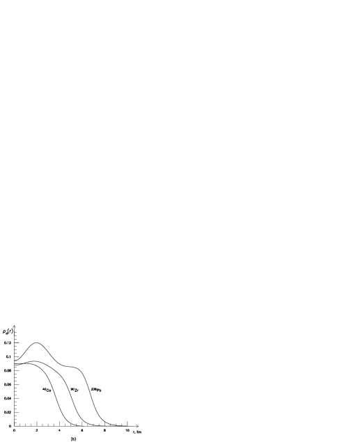
Figure 7: Density distributions of protons (a) and neutrons (b) in ⁴⁰Ca, ⁹⁰Zr and ²⁰⁸Pb nuclei.

The data of Ref. [2] are based on high precision measurements of elastic electron-nucleus scattering thus providing the proton density distributions in the whole nuclear region. The situation for the neutron densities is different since the elastic 1 GeV proton-nucleus scattering underlying the data of Ref. [3] is sensitive mainly to the surface region of nucleus because of the absorption. For this reason the neutron density distributions $\rho_{n}(r)$ may differ from the Woods–Saxon–like ones of Ref. [3] in nuclear interior (as seen from Fig. 7a the proton densities are indeed different from the Woods–Saxon-like ones). The latter is just the region to which the doorway state energies are sensitive, and therefore they may be used to specify the Ref. [3] data for the neutron densities. We looked for the latter ones in the form

$$\rho_{n}(r)\ =\ \rho_{0}\bigg{[}W_{A}(r)+\alpha W_{A}(0)\varphi_{4}(\beta r)\bigg{]}\ ,$$ (41)

where $W_{A}(r)$ are the deconvoluted neutron densities of Ref. [3] and $\varphi_{4}(x)$ is the fourth Hermite function. The neutron density parameters $\alpha,\beta$ and the strength ones $a_{3},a_{4},a^{-}_{3},a^{-}_{4}$ are determined from the best fit for both the doorway state energies and the elastic 1 GeV proton-nucleus scattering, the latter being calculated within the Glauber theory [16].

Table 1: Neutron density parameters

	Bonn $B$		OSBEP
	$\alpha$	$\beta$	$\alpha$	$\beta$
40Ca	$-0.0295$	0.5314	$-0.0255$	0.5230
90Zr	$-0.0758$	0.5551	$-0.0646$	0.5442
208Pb	$-0.2645$	0.5445	$-0.2667$	0.5389

The density parameters are shown in Table 1. They are different for the two choices of the two-particle forces, but the difference is rather small. For this reason neither the resulting neutron density distributions, Fig. 7b, nor the 1 GeV proton–nucleus elastic scattering cross sections, Fig.8, are distinguishable in the figures. We also calculated the proton–nucleus cross sections with the original results of Ref.[3] for the density distributions.

 

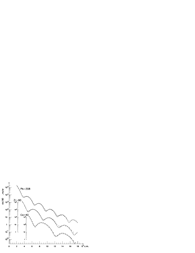
Figure 8: 1 GeV proton-nucleus elastic scattering cross sections. The dashed and full curves are calculated with the original neutron density distributions of Ref. [3] and the specified ones respectively.

As seen from Fig.8 the agreement with experiment is equally good for both the specified densities, Eq.(41), and the original ones. The many–particle strength parameters are

$$a_{3}=16.9296\mbox{ fm}^{5}\ , a_{4}=-107.6744\mbox{ fm}^{8}\ ,$$

$$a^{-}_{3}=25.5873\mbox{ fm}^{5}\ , a^{-}_{4}=-128.5134\mbox{ fm}^{8}$$ (42)

for the Bonn $B$ two-particle forces and

$$a_{3}=17.0011\mbox{ fm}^{5}\ , a_{4}=-110.3747\mbox{ fm}^{8}\ ,$$

$$a^{-}_{3}=26.9036\mbox{ fm}^{5}\ , a^{-}_{4}=-130.1210\mbox{ fm}^{8}$$ (43)

for the OSBEP ones. As seen from Eqs. (42) and (43) the strength parameters of the free-space many-particle forces are almost the same for the two cases. This is not surprising because both the Bonn $B$ and the OSBEP potentials provide an equally good description of the two-nucleon data, see the discussion in the Introduction.

The results including both the contribution from the many-particle forces and the specified neutron densities are labelled as ”full” in Figs. 4 and 5. The ”full” doorway state energies agree with the observed ones (which are labelled as ”exp”) within the experimental error of 3 MeV. The exception is provided by the $2s_{1/2}$ states in ²⁰⁸Pb: in this case the discrepancy is about 5 MeV. The reason is not clear yet, but the discrepancy does not exceed two experimental errors.

To estimate the relative importance of the two-particle and many-particle contributions to the static field of nucleus let us perform the calculations for nuclear matter, see Sect.3. First consider the isoscalar part. The two-particle contribution is

$$U_{2}=V_{2}+S_{2}=\hbar c\left[v_{\omega}(0)\rho-\left(\frac{3}{4}v_{\sigma 1}(0)+\frac{1}{4}v_{\sigma 0}(0)\right)\rho_{s}\right]=\left\{{-83\mbox{ MeV},\ \mbox{ Bonn }B\atop-82\mbox{ MeV},\ \mbox{ OSBEP },}\right.$$ (44)

whereas those from three-particle and four-particle forces are

$$U_{3} = \hbar ca_{3}\rho^{2}=\left\{{96.5\mbox{ MeV,~{}~{}~{} Bonn }B\atop 97\mbox{ MeV,~{}~{}~{} OSBEP}}\right.$$

$$U_{4} = \hbar ca_{4}\rho^{3}=\left\{{-104\mbox{ MeV,~{}~{} Bonn }B\atop-107\mbox{ MeV,~{}~{} OSBEP}}\right.$$ (45)

the many-particle contributions thus being as large as the two-particle one.

The isovector part may be estimated by putting $\rho^{-}=\frac{N-Z}{A}\rho$ and $\rho^{-}_{s}=\frac{N-Z}{A}\rho_{s}$. The two-particle contribution is (see Sect.3)

$$U^{-}_{2} = \hbar c\left[v_{\rho}(0)\rho^{-}-\left(v_{\delta}(0)+\frac{1}{4}v_{\sigma 1}(0)-\frac{1}{4}v_{\sigma 0}(0)\right)\rho^{-}_{s}\right]\ =$$ (46)

$$= {6\frac{N-Z}{A}\mbox{ MeV,~{}~{}~{} Bonn }B\atop 0.15\frac{N-Z}{A}\mbox{ MeV,~{} OSBEP}}$$

the many-particle one being

$$U^{-}_{m}=\hbar c\left(a^{-}_{3}\rho+a^{-}_{4}\rho^{2}\right)=\left\{\begin{array}[]{ll}\displaystyle(146-125=21)\frac{N-Z}{A}\mbox{ MeV,}&\mbox{ Bonn }B\\ \displaystyle(153-126=27)\frac{N-Z}{A}\mbox{ MeV,}&\mbox{ OSBEP }.\end{array}\right.$$ (47)

So the many-particle forces provide the dominant part of the isovector nuclear potential. The reason is due to the fact that the two-particle contribution arises from the exchange by isovector mesons $\rho$ and $\delta$ which are weakly coupled to nucleon, see Table 5 of Ref.[11] and Table 1 of Ref.[12].

5 Summary

The above results give rise to the following general conclusions:

1. Our results for the many-particle forces are quite competitive with those from the few-nucleon systems [17]. Indeed, the properties of the latter ones (binding energies, sizes, formfactors etc.) are expressed through the interaction in all orders of the perturbation theory, and therefore the solution of a rather complicated quantum mechanical problem is necessary to get the information on the many-particle forces. In contrast to the few-nucleon systems the doorway states for the one-nucleon transfer reactions in complex nuclei are solutions of a much more simple problem for one nucleon in central field. In addition the static nuclear field is expressed through the $NN$ forces in first order of the perturbation theory, the results thus being very visual, see Figs. 1 and 6. The information from the doorway states is, however, restricted because it concerns only spin-independent terms of the many-particle forces (the spin-dependent ones do not contribute to the Hartree diagrams). Nevertheless it is a useful addition to that from the few-nucleon systems.

Two important points should be mentioned in this connection. (i) Only three-particle forces (in addition to the two-particle ones) are included in all available calculations for the few-nucleon systems. Our results clearly show that this is insufficient. (ii) Calculating the nuclear correlation effects (binding energies and rms radii of finite nuclei, equation of state of nuclear matter, etc.), with the free-space $NN$ interaction there is no reason to neglect the many-particle forces because they are as strong as the two-particle ones, compare Eqs. (44) and (45).

2. The effective three-particle and four-particle forces are also repulsive and attractive respectively in the recent calculations within the relativistic mean-field approximation [18, 19], see the Appendix. Such forces include implicity the correlation effects which are not taken into account explicitly within this framework. For this reason the above signs of the forces might be treated as the artifact of the approximation. But our results for the free-space many-particle forces show that this is not the artifact.

Appendix A Appendix

The potential energy of the $\sigma$ mesons is [18, 19]

$$U(\sigma)\ =\ \frac{\mu^{2}}{2}\ \sigma^{2}+\frac{\lambda_{3}}{3}\ \sigma^{3}+\frac{\lambda_{4}}{4}\ \sigma^{4}$$ (A.1)

with $\lambda_{3}<0$ and $\lambda_{4}<0$, the scalar field $S=g\sigma$ thus obeying the equation

$$(\Delta-\mu^{2})S\ =\ g^{2}_{\sigma}\rho_{s}+\frac{\lambda_{3}}{g}\ S^{2}+\frac{\lambda_{4}}{g^{2}}\ S^{3}\ .$$ (A.2)

Let us use the following iteration procedure

$$(\Delta-\mu^{2})S_{n}\ =\ g^{2}_{\sigma}\rho_{s}+\frac{\lambda_{3}}{g}S^{2}_{n-1}+\frac{\lambda_{4}}{g^{2}}S^{3}_{n-1}$$ (A.3)

with

$$(\Delta-\mu^{2})S_{0}\ =\ g^{2}_{\sigma}\rho_{s}$$ (A.4)

for the initial iteration. The result is

$$S(r) = -g^{2}\int y(|{\bf r}-{\bf r}_{1}|)\rho^{(r)}_{s}(r_{1})d^{3}{\bf r}_{1}\quad+$$

$$+ \int f_{3}(|{\bf r}-{\bf r}_{1}|,|{\bf r}-{\bf r}_{2}|)\rho_{s}(r_{1})\rho_{s}(r_{2})d{\bf r}_{1}d{\bf r}_{2}\ +$$

$$+ \int f_{4}(|{\bf r}-{\bf r}_{1}|,|{\bf r}-{\bf r}_{2}|,|{\bf r}-{\bf r}_{3}|)\rho_{s}(r_{1})\rho_{s}(r_{2})\rho_{s}(r_{3})d^{3}{\bf r}_{1}d^{3}{\bf r}_{2}d^{3}{\bf r}_{3}\ +\ \cdots\ ,$$

where

$$y(|{\bf r}-{\bf r}^{\prime}|)\ =\ \frac{\exp(-\mu|{\bf r}-{\bf r}^{\prime}|)}{4\pi|{\bf r}-{\bf r}^{\prime}|}$$

$$f_{3}(|{\bf r}-{\bf r}_{1}|,|{\bf r}-{\bf r}_{2}|)\ =\ -\lambda_{3}g^{3}\int y(|{\bf r}-{\bf r}^{\prime}|)y(|{\bf r}_{1}-{\bf r}^{\prime}|)y(|{\bf r}_{2}-{\bf r}^{\prime}|)d^{3}{\bf r}^{\prime}$$

$$f_{4}(|{\bf r}-{\bf r}_{1}|,|{\bf r}-{\bf r}_{2}|,|{\bf r}-{\bf r}_{3}|)\quad=$$

$$= \lambda_{4}g^{4}\int y(|{\bf r}-{\bf r}^{\prime}|)y(|{\bf r}_{1}-{\bf r}^{\prime}|)y(|{\bf r}_{2}-{\bf r}^{\prime}|)y(|{\bf r}_{3}-{\bf r}^{\prime}|)d^{3}r^{\prime}\ -$$

$$- 2\lambda^{2}_{3}g^{4}\int y(|{\bf r}-{\bf r}^{\prime}|)y(|{\bf r}_{1}-{\bf r}^{\prime}|)y(|{\bf r}^{\prime}-{\bf r}^{\prime\prime}|)y(|{\bf r}_{2}-{\bf r}^{\prime\prime}|)y(|{\bf r}_{3}-{\bf r}^{\prime\prime}|)d^{3}{\bf r}^{\prime}d^{3}{\bf r}^{\prime\prime}.$$

The dots in the rhs of Eq.(A.5) represent the higher-power terms in respect of $\rho_{s}$ resulting from the higher many-particle forces. As seen from (A.7) the three-particle force is repulsive because of the sign of $\lambda_{3}$ ($g>0$ in Refs.[18, 19]). The four–particle one, Eq.(A.8), consists of two terms. The first is of first order with respect to the $\lambda_{4}$ term of (A.1). It is attractive because of the sign of $\lambda_{4}$. The second is of second order with respect to the $\lambda_{3}$ term. It is attractive irrespective of the sign of $\lambda_{3}$.

The volume integrals of the forces (A.7) and (A.8), Eqs. (37) and (38), are

$$a_{3}\ =\ -g^{3}\lambda_{3}\mu^{-6},\quad a_{4}\ =\ g^{4}(\lambda_{4}-2\lambda^{2}_{3}\mu^{-2})\mu^{-8}\ .$$ (A.9)

The least values of these quantities correspond to the NL-SH parameter set of Ref.[18], Table 2 of this reference. They are

$$a_{3}\ =\ 21.9\mbox{ fm}^{5}\ ,\quad a_{4}\ =\ -136.5\mbox{ fm}^{8}\ ,$$ (A.10)

thus being rather close to the free-space values, Eqs. (42) and (43).

References

• [1] M. Baranger, Nucl.Phys. A149 (1970) 225.
• [2] H. de Vries et al. At. Data and Nucl. Data Tables 36 (1987) 495.
• [3] G.D. Alkhazov et al. Nucl.Phys. A381 (1982) 430.
• [4] A.A. Abrikosov, L.P. Gor’kov and I.E.Β Dzyaloshinski ”Methods of quantum field theory in statistical physics” M, 1962.
• [5] A.B. Migdal ”Finite Fermi-system theory and properties of atomic nuclei” M. 1983.
• [6] S.G. Kadmenski and P.A. Lukyanovich, J.Nucl.Phys. 49 (1989) 1295.
• [7] S.S. Volkov et al., J.Nucl.Phys. 53 (1990) 1339.
• [8] A.A. Vorobyov et al., J.Nucl.Phys. 58 (1995) 1923.
• [9] K. Erkelenz, Phys.Reports 13 (1974) 191.
• [10] M. Lacombe, Phys.Rev. C21 (1980) 861.
• [11] R. Machleidt, K. Holinde and Ch.Β Elster, Phys.Reports 149 (1987) 1.
• [12] L. JΓ€de and H.V. von Geramb, Phys.Rev. C57 (1998) 496.
• [13] R. Machleidt, Adv. in Nucl.Phys. 19 (1989) 189.
• [14] J.D. Walecka, Ann. of Phys. (NY) 83 (1974) 491.
• [15] S.J. Wallace, Comments on Nucl. and Part.Phys. 13 (1984) 27.
• [16] R.J. Glauber, ”Lectures in theoretical physics”, ed. W.E.Β Brittin et al., vol.1 (NY 1959).
• [17] R. Schiavilla, V.R. Pandharipande and R.B.Β Wiringa, Nucl.Phys. A449 (1986) 219.
• [18] G.A. Lalazissis, J. KΓΆnig and P.Β Ring, Phys.Rev. C55 (1997) 540.
• [19] M.L. Cescato and P. Ring, Phys.Rev. C57 (1998) 134.