Multiple pion production from an oriented chiral condensate

Abstract

We consider an “oriented” chiral condensate produced in the squeezed states of the effective field theory with time- and space-dependent pion mass parameter. We discuss the general properties of the solution, identifying condensate modes and determining the resulting pion distributions. The implementation of the dynamics in the form of sudden perturbation allows us to look for exact solutions. In the region of condensation, the dramatic increase in pion production and charge fluctuations are demonstrated.

I Introduction

Pions have always played an important role in heavy ion reactions. With their relatively strong coupling to nuclei and very small mass, pions can be produced in large quantities and can carry important detectable information about the state of nuclear matter during the reaction. Large fluctuations in the ratio of charged to neutral pions have been observed in cosmic ray experiments [1] and have recently been a subject of many discussions. The major interest in this direction is motivated by an almost a decade old idea [2, 3, 4] that at high enough energies the pion-sigma ground state symmetry breaking condensate can be destroyed. In the latter process of sudden cooling there is a chance of the formation of disoriented chiral domains, given that the terms responsible for the explicit breaking of chiral symmetry are small. The formation of this disoriented chiral condensate (DCC) is presumably responsible for the observed discrepancy in the ratio of pion species. Further enthusiasm about these ideas is generated by the fact that it may be possible to achieve an environment capable of producing disoriented chiral domains in relativistic heavy ion collisions. In that case the large fluctuations in pion types can be a signal of a DCC.

There exist a number of theoretical works investigating the production and development of DCCs in heavy ion collisions. The assumption of a random equiprobable orientation of the pionic isovector leads [3] to the probability of observing a fraction of neutral pions $f\equiv N_{\pi^{0}}/(N_{\pi^{+}}+N_{\pi^{-}}+N_{\pi^{0}})$ being

$${\cal P}(f)={1\over 2\sqrt{f}}\,.$$ (1)

This result is consistent with the slowly varying classical pionic field as a solution of the non-linear $\sigma$-model [5]. It can also be obtained as a limiting large $N$ distribution in the coherent single-mode pion production by an isoscalar operator [6, 7, 8]

$$\left({\vec{a}}\,^{\dagger}\cdot{\vec{a}}\,^{\dagger}\right)^{N/2}\,=\,\left(a^{\dagger}_{x}a^{\dagger}_{x}+a^{\dagger}_{y}a^{\dagger}_{y}+a^{\dagger}_{z}a^{\dagger}_{z}\right)^{N/2}\,.$$

The formation and the nature of domain structures is an important question in itself [9, 10]. In the case of many small domains or in the absence of a DCC, one would expect a Gaussian distribution $P(f)\,,$ following from the central limit theorem. More complicated methods of quantum and classical field theory applied to this problem with different assumptions of formation, evolution [11, 12] and dissociation of DCCs [13, 14] lead to different results. Pionic mode mixing and final state interaction may also greatly change the observed forms of these probability distributions [8, 5, 15].

Most of the existing theoretical works consider pion production from DCC domains formed in the dynamical process of symmetry restoration and later sudden relaxation into a non-symmetric vacuum which is some times called quench [16]. The word “disoriented” also describes the theoretical foundation of the DCC approach which is based on introducing an effective disoriented current-type term in the Lagrangian. The advantage of this formalism is in the simplicity of the solution, as a current-type interaction can always be solved with a coherent state formalism [17]. In contrast to that the linear sigma model, a well-established effective theory based on chiral symmetry, naturally leads to a quadratic pion field term in the Lagrangian. The goal of the present work is to consider an “oriented” chiral condensate with a chirally symmetric Lagrangian that to the lowest order is quadratic in the pion field. Throughout all this paper we are going to deal with the wave equation for pions in the form

$${\partial^{2}\vec{\pi}\over\partial t^{2}}-\nabla^{2}\vec{\pi}+m_{\rm eff}^{2}({\bf x},t)\,\vec{\pi}=0\,.$$ (2)

This is the equation of motion deduced from a quadratic Lagrangian. Equation (2) contains an effective mass $m_{\rm eff}({\bf x},t)$ which is due to a mean field from non-pionic degrees of freedom. This term produces a parametric excitation of the pionic field, and, if $m^{2}_{\rm eff}<0$, may lead to amplification of low momentum modes and the formation of a chiral condensate. The chiral condensate in this picture is “oriented”; as opposed to the usual picture of a DCC. The scalar mean field (effective mass) introduced here does not break the symmetry properties of pion fields in any way. The quantum problems formulated by equations of the form (2) address a variety of physical issues, and can be encountered in different areas of physics. In general, such non-stationary quantum problems cannot be solved exactly. Even studies with approximate methods like perturbation theory, impulse approximations, adiabatic expansions and many others often require sophisticated approaches. We will address those rare occasions when exact solutions may be obtained. The significance of the analytical solution should not be underestimated. The exact results could exhibit the unperturbative features of the solutions, like phase transitions and condensates, as well as point the way to a good approximate theory.

The paper is structured as follows. We start with a short introduction to the linear sigma model and show that effectively it leads to Eq. (2) for a pion field. In the next section we discuss an exact solution of Eq. (2). First, we show that from the classical solution a quantum solution can be built exactly. Then, based on the general form of the evolution matrix, we obtain and discuss possible forms of the multiplicity distribution. The bulk of the paper is concentrated in Sec. IV. where we further analyze the properties of the solutions to Eq. (2). By considering a simpler model of space-independent but variable-in-time effective mass we clearly define the exponentially growing “condensate” momentum modes. Depending on the number and strength of the condensate modes we obtain different distributions for a particle number and distributions over pion species. We emphasize the limits when Eq. (1) is recovered or when ${\cal P}(f)$ becomes Gaussian. In the following part of Sec. IV we consider a full field equation with a time- and space-dependent mass parameter and address the exactly solvable case of a mass parameter abruptly changing and returning to normal. We show that in this picture the condensate modes are still identifiable and they still have a characteristic momentum distribution. Final summary and conclusions are given in Sec. V.

II The Linear sigma model

Below we give a short review of the linear sigma model, point out the origin of Eq. (2) in the context of pion fields and deliberate the possible form of the effective mass term. We assume the usual linear sigma model Lagrangian of the pion and sigma fields [18]

$${\cal L}_{L.S.}={1\over 2}\left(\partial_{\mu}{\vec{\pi}}\right)\cdot\left(\partial^{\mu}{\vec{\pi}}\right)+{1\over 2}\left(\partial_{\mu}\sigma\right)\,\left(\partial^{\mu}\sigma\right)-{\lambda\over 4}\left(({\vec{\pi}}^{2}+\sigma^{2})-v_{0}^{2}\right)^{2}+\epsilon\sigma\,,$$ (3)

where explicit symmetry breaking is introduced by the parameter $\epsilon$. The sigma field has a non-zero vacuum expectation value $f_{\pi}$ that is set by the Goldberger-Treiman relation and is related to the above mentioned symmetry breaking parameter as

$$v_{0}^{2}=f_{\pi}^{2}-{\epsilon\over\lambda f_{\pi}}\,.$$

The Lagrangian of Eq. (3) produces the following masses of the pion and sigma mesons

$$m_{\pi}^{2}={\epsilon\over f_{\pi}}\,,\qquad m_{\sigma}^{2}=2\lambda f_{\pi}^{2}+{\epsilon\over f_{\pi}}\,.$$

Equations of motion for each isospin component of the pion field $\pi_{\tau}$ have the form

$${\partial^{2}\pi_{\tau}\over\partial t^{2}}-\nabla^{2}\pi_{\tau}+\lambda\left(({\vec{\pi}}^{2}+\sigma^{2})-v_{0}^{2}\right)\pi_{\tau}=0\,.$$ (4)

In the mean field approximation non-pionic degrees of freedom, like the sigma field, are approximated by their expectation value. Then the dynamics of the pionic field can be viewed as a field equation of type (2), with a time- and space-dependent mass parameter

$$m_{\rm eff}^{2}({\bf x},t)=\lambda\left(\langle{\vec{\pi}}^{2}+\sigma^{2}\rangle-v_{0}^{2}\right)\,.$$

As in the application to the chiral condensates, we would like to solve Eq. (4) in the formalism of quantum field theory with reasonable expectation values $\langle{\vec{\pi}}^{2}+\sigma^{2}\rangle$. We do not solve the problem self-consistently because $m_{\rm eff}({\bf x},t)\,,$ being generated by other degrees of freedom, is placed in by hand as a mean field. Before and long after the reaction the fields are in their ground state so that $\langle\pi_{\tau}\rangle=0$ and $\langle\sigma\rangle=f_{\pi}$ , which is equivalent to

$$m^{2}_{\rm eff}({\bf x},t=-\infty)=m^{2}_{\rm eff}({\bf x},t=+\infty)=m^{2}_{\pi}\,.$$

During the reaction, the behavior of the effective mass is unknown, and in our case would be an input to the model. When chiral symmetry is restored the expectation of the $\sigma$ field tends to zero, while the effective squared pion mass is positive. A sudden return of the effective potential to its vacuum form (quenching) can strand the $\sigma$ mean field near zero with a large negative value of the effective pion mass squared, which in the extreme limit would reach $m_{\rm eff}^{2}=-\lambda v_{0}^{2}\approx-m_{\sigma}^{2}/2\,.$ A negative value of $m_{\rm eff}^{2}$ would lead to an exponential growth of the low momentum pion modes and long range correlations, i.e. the creation of a chiral condensate [19].

III From classical to quantum solutions

The generic form of the Lagrangian density of the field $\psi$ that has field terms up to the second order in its potential energy part is

$${\cal L}={1\over 2}\left(\partial_{\mu}{\psi}\right)\,\left(\partial^{\mu}{\psi}\right)-J({\bf x},t)\,\psi-{1\over 2}m^{2}({\bf x},t)\,\psi^{2}\,.$$ (5)

To clarify the approach, we consider here a bosonic isoscalar field $\psi\,.$ This does not limit the consideration and will be generalized later. It is known that the linear terms $J({\bf x},t)$, often called a current or force, can always be removed from consideration [20]. The time-dependent current term is responsible for the creation of coherent states with a Poissonian distribution of particles. Intensive studies of a DCC produced by linear-type coupling of the pions to the disoriented mean field have been performed [15]. Unfortunately, many problems cannot be easily reduced to this linear approximation. As mentioned in the Introduction, for the chiral condensate this would require the Introduction of a symmetry breaking isovector current ${\vec{J}}({\bf x},t)$, whereas introducing a scalar effective mass (a quadratic term in the Lagrangian) preserves intrinsic symmetries.

There is one important feature of the problem with a quadratic perturbation in the Lagrangian. The equations of motion for the field, like Eq. (2), are linear for the Lagrangian (5); therefore they are identical for the classical fields and the corresponding operators in the Heisenberg picture. Thus, an exact classical solution is related to the solution to the quantized version of the problem. The step from classical to quantum treatment will be considered next.

A Parametric excitation of a harmonic oscillator

The parametric excitation of a quantal harmonic oscillator has been extensively considered in the literature starting from refs. [21, 22, 23]. This corresponds to our problem in the case of no spatial dependence of the effective mass. The presence of translational symmetry in this case leads to the conservation of linear momentum. The quantum number of momentum, $k$, can be used to label the normal modes. Each mode is just a simple oscillator with the time-dependent frequency. The simple Fourier transformation from $x$ to $k$ transforms the Hamiltonian, that corresponds to the Lagrangian in Eq. (5), into a sum over modes (for simplicity we keep one-dimensional notations)

$$H={1\over 2}\int\,dx\,\left(\dot{\psi}(x,t)^{2}+\nabla^{2}\psi(x,t)+m^{2}_{\rm eff}(t)\psi^{2}(x,t)\right)={1\over 2}\sum_{k}\left(\dot{\psi_{k}}^{2}+k^{2}\,\psi_{k}^{2}+m^{2}_{\rm eff}(t)\psi_{k}^{2}\,\right).$$ (6)

With this reduction we arrive at the problem of the independent development of a large number of quantum oscillators. With the notation $\omega^{2}_{k}(t)=m^{2}_{\rm eff}(t)+k^{2}\,,$ we have a classical equation of motion for each mode $k$

$$\ddot{\psi_{k}}+\omega^{2}_{k}(t)\psi_{k}=0\,.$$ (7)

After the quantization, the $\psi_{k}$ and the corresponding momenta become operators. Assuming a particular normal mode $k$ below we omit this subscript.

Even for the problem of a simple oscillator, the relation between the classical and quantum solution is quite subtle; not to mention that classically Eq. (7) is analogous to a standard problem in quantum mechanics of scattering from a potential $-\omega^{2}$ that is known to have only a limited number of cases with exact analytical solutions.

Classically, the $S$-matrix would be defined if we assume that a solution of Eq. (7) with the asymptotics in the remote past corresponding to the frequency $\omega_{-}\,,$

$$\psi(t)=e^{-i\,\omega_{-}t}\,\quad{\rm at}\quad t\rightarrow-\infty\,,$$ (8)

has evolved with time to a final general form of the solution with the frequency $\omega_{+}\,,$

$$\psi(t)=\,\sqrt{\omega_{-}\over\omega_{+}}\left(u\,e^{-i\,\omega_{+}t}\,+\,v^{*}\,e^{+i\,\omega_{+}t}\right)\,\quad{\rm at}\quad t\rightarrow+\infty\,.$$ (9)

It is clear that the complex conjugate to Eq. (8) will develop into a corresponding complex conjugate version of Eq. (9). Furthermore, the unitarity, i.e. conservation of probability applied to Eq. (7), results in a restriction posed on $u$ and $v$

$$|u|^{2}\,-\,|v|^{2}\,=\,1\,.$$ (10)

In order to analyze the quantum version of the problem we use the language of secondary quantization, introducing creation and annihilation operators for a single harmonic oscillator. The time dependence of a quantized field coordinate $\psi(t)$ in the Heisenberg representation as $t\,\rightarrow\,-\infty$ is

$$\psi(t)\,=\,{1\over\sqrt{2\omega_{-}}}\left(a\,e^{-i\,\omega_{-}t}\,+\,a^{\dagger}\,e^{i\,\omega_{-}t}\right)\,,$$ (11)

where the operators $a$ and $a^{\dagger}$ do not depend on time and define the “in” state of the system. We will define the “out” state using operators $b$ and $b^{\dagger}$ as

$$\psi(t)\,=\,{1\over\sqrt{2\omega_{+}}}\left(b\,e^{-i\,\omega_{+}t}\,+\,b^{\dagger}\,e^{i\,\omega_{+}t}\right)\,\quad{\rm at}\quad t\,\rightarrow\,+\infty\,.$$ (12)

Being supported by the fact that the field $\psi(t)$, even in its quantum form, satisfies Eq. (7), and with our assumptions about the classical solution (8, 9) we can relate operators $a$ and $a^{\dagger}$ with $b$ and $b^{\dagger}\,,$

$$b\,=\,\left(u\,a+v\,a^{\dagger}\right)\,,\quad b^{\dagger}\,=\,\left(u^{*}\,a^{\dagger}+v^{*}\,a\right)\,,$$ (13)

with the same parameters $u$ and $v$ as in the classical solution. As seen (13) the “in” and “out” states are related by a Bogoliubov transformation. The condition that the commutation relation

$$[b,b^{\dagger}]\,=\,(|u|^{2}-|v|^{2})\,[a,a^{\dagger}]\,=\,1$$

is preserved coincides with Eq. (10) .

It is possible to build an $S$-matrix corresponding to the transformation in Eq. (13), however the solution is very technical, and of limited use. We can use Eq. (13) directly to answer simple but relevant questions. The probability amplitude to have $n$ final quanta if there was vacuum in the initial state is given by

$$C_{n}\,=\,_{a}\langle n|S|0\rangle_{a}\,=\,_{a}\langle n|0\rangle_{b}\,,$$

where the $S$-matrix is a transition matrix from the “in” state to the “out” state. Then

$$|0\rangle_{b}\,=\,\sum_{n=0}^{\infty}\,C_{n}|n\rangle_{a}\,,$$

and recursion relation for the coefficients $C_{n}$

$$C_{n+2}=-{v\over u}\,\sqrt{n+1\over n+2}\,C_{n}\,$$ (14)

may be found from the definition of the vacuum and Eq. (13):

$$b|0\rangle_{b}\,=\,\sum_{n=0}^{\infty}C_{n}\,\left(u\,\sqrt{n}\,|n-1\rangle_{a}+v\,\sqrt{n+1}\,|n+1\rangle_{a}\right)\,=\,0\,.$$

Finally, normalized to unity, the transition probability from a vacuum to a state with $2n$ bosons is expressed by

$$|C_{2n}|^{2}\,\equiv\,P(2n)\,=\,{(2n)!\over 2^{2n}\,(n!)^{2}}\,\rho^{n}\,\sqrt{1-\rho}\,,$$ (15)

where the parameter $\rho=|v/u|^{2}$ represents the reflection probability for Eq. (7) if it is viewed as a Schrödinger equation for scattering at zero energy off a potential $-\omega^{2}\,.$ Conservation of probability, Eq. (10), limits the values of $\rho$ to the region $\rho\in[0,1)\,.$ The distribution of particles produced from vacuum Eq. (15) peaks at zero and the average number of particles produced is

$$\overline{n}\,=\,\sum_{n=0}^{\infty}\,2n\,P(2n)\,=\,{\rho\over 1-\rho}\,.$$ (16)

It is seen from the above expression that the number of particles diverges as $\rho$ approaches one. This will be a region of interest in our later studies of chiral condensates.

A rigorous and detailed discussion of all the features in the transition from classical solutions of Eq. (7) to a problem of a quantum oscillator with a time-dependent frequency can be found in [21, 22, 23]. The corresponding Schrödinger equation for the wave function of the quantum oscillator is ($\hbar=1$)

$$i\,{\partial\Phi(x,t)\over\partial t}\,=\,-\,{1\over 2}\,{\partial^{2}\Phi(x,t)\over\partial x^{2}}+{1\over 2}\,\omega^{2}(t)\,x^{2}\,\Phi(x,t)\,,$$ (17)

where coordinate $x$ originates from the field “coordinate” $\psi$, Eq. (7). Let some function $\psi(t)$ be a solution to classical Eq. (7) with $\omega(t=-\infty)=\omega_{-}$ and $\omega(t=+\infty)=\omega_{+}$. This function $\psi(t)$ can be written in terms of the real part $r(t)$ and phase $\gamma(t)$ so that $\psi(t)=\,r(t)\,e^{i\gamma(t)}\,.$ With a direct substitution it can be shown that

$$\Phi(x,t)={1\over\sqrt{r(t)}}\,\exp{\left(i{\dot{r}x^{2}\over 2r}\right)}\,\chi(y,\tau)$$ (18)

is a solution to the quantum equation (17). Here a rescaled length $y$ and time $\tau$ are introduced as $y=x/r(t)\,,$ $\tau=\gamma(t)/\omega_{-}$. The function $\chi(x,t)$ is a standard solution of the Schrödinger equation for the oscillator with a constant frequency $\omega_{-}\,,$

$$i\,{\partial\chi(y,\tau)\over\partial\tau}\,=\,-\,{1\over 2}\,{\partial^{2}\chi(y,\tau)\over\partial y^{2}}+{1\over 2}\,\omega_{-}\,y^{2}\,\chi(y,\tau)\,.$$ (19)

The initial conditions for the solution $\chi(y,\tau)$ should be set at $t\rightarrow-\infty$ by the known conditions on $\Phi(x,t)\,.$ Equation (15) can be generalized utilizing this more general technique. It can be shown that the probability for a transition from the state with $m$ quanta into the final state of $n$ quanta is given by

$$\,{\min(m,n)!\over\max(m,n)!}\sqrt{1-\rho}\left|P_{(m+n)/2}^{|m-n|/2}(\sqrt{1-\rho})\right|^{2}\,,$$ (20)

where $P_{\nu}^{\mu}$ are the associated Legendre polynomials and $n$ and $m$ have to be of the same parity. The established bridge between classical and quantum solutions is a remarkable achievement, but unfortunately analysis of Eq. (18) does not present a pleasant task.

B Infinite number of mixed modes

1 General canonical transformation

The situation becomes more complicated if we return to the general field equation given by the Lagrangian density of Eq. (5), and assume that the modes cannot be separated. We keep assuming $J(x,t)=0$ which is relevant to our particular problem but in general this factor can be included back in the discussion without much complication. The problem of the system of coupled oscillators has been discussed in great detail in [24]. The transformation analogous to Eq. (13) now takes an $N$-dimensional symplectic form, where $N$ is the number of coupled modes [25],

$$b_{k}\,=\,\sum_{k^{\prime}=1}^{N}\,\left(u_{k\,k^{\prime}}\,a_{k^{\prime}}+v_{k\,k^{\prime}}\,a_{k^{\prime}}^{\dagger}\right)\,,\quad b_{k}^{\dagger}\,=\,\sum_{k^{\prime}=1}^{N}\,\left(u_{k\,k^{\prime}}^{*}\,a_{k^{\prime}}^{\dagger}+v_{k\,k^{\prime}}^{*}\,a_{k^{\prime}}\right)\,,$$ (21)

It is convenient to regard the operators $a_{k}$ as components of an $N$-dimensional vector, and the numbers $u_{k\,k^{\prime}}$ and $v_{k\,k^{\prime}}$ as $N\times N$ matrices. Eq. (21) in matrix notation takes the form

$$b\,=S^{-1}\,a\,S\,=\,u\,a\,+\,v\,a^{\dagger}\,,\quad b^{\dagger}\,=\,S^{-1}\,a^{\dagger}\,S\,=\,u^{*}\,a^{\dagger}\,+\,v^{*}\,a\,.$$ (22)

Using the properties of the matrices $u$ and $v$ shown below, it is straightforward to check that the inverse transformation is given by

$$a\,=S\,b\,S^{-1}\,=\,u^{\dagger}\,b\,-\,v^{T}\,b^{\dagger}\,,\quad a^{\dagger}\,=\,S\,b^{\dagger}\,S^{-1}\,=\,u^{T}\,b^{\dagger}\,-\,v^{\dagger}\,b\,,$$ (23)

where $u^{*}$, $u^{\dagger}$ and $u^{T}$ have their usual meanings of complex conjugate, hermitian conjugate and transpose matrices, respectively. Further, we will also use an inversion denoted as $u^{-1}\,.$ Similarly to the one-mode example of Eq. (10), matrices $u$ and $v$ are subject to conditions that arise from the fact that the commutation relations have to be preserved. It follows from Eq. (22) that

$$u\,u^{\dagger}\,-\,v\,v^{\dagger}\,=\,1\,,\quad u\,v^{T}\,-\,v\,u^{T}=0\,,$$ (24)

and from the inverse transformation, Eq. (23)

$$u^{\dagger}\,u\,-\,v^{T}\,v^{*}\,=\,1\,,\quad u^{\dagger}\,v\,-\,v^{T}\,u^{*}=0\,.$$ (25)

2 Transitions between coherent states

In the case of many mixed modes it is still possible to obtain recursion relations similar to the single-mode situation of Eq. (14) but they become difficult to analyze. Next we will discuss the approach found in [24] with a different technique that uses the transitions between coherent states. We define a single-mode coherent state $|\alpha\rangle$ in the usual way as

$$|\alpha\rangle\,=\,e^{-|\alpha|^{2}/2}\,\sum_{n=0}^{\infty}\,{\alpha^{n}\over\sqrt{n!}}|n\rangle\,.$$ (26)

In mathematics sums as in Eq. (26) are often called generating functions. It is convenient to introduce states with a different normalization [26] as

$$||\alpha\rangle\,=\,e^{|\alpha|^{2}/2}\,|\alpha\rangle\,=\,e^{\alpha\,a^{\dagger}}\,|0\rangle\,.$$ (27)

When applied to the states (27), the creation operation is equivalent to the derivative,

$$a^{\dagger}\,||\alpha\rangle\,=\,{\partial\over\partial\alpha}\,||\alpha\rangle\,.$$ (28)

We continue to use the notation $|\mathchoice{{\hbox{\boldmath$\displaystyle\alpha$}}}{{\hbox{\boldmath$\textstyle\alpha$}}}{{\hbox{\boldmath$\scriptstyle\alpha$}}}{{\hbox{\boldmath$\scriptscriptstyle\alpha$}}}\rangle$ for a multidimensional coherent state, which should be interpreted as a product of the single-mode states. $\textstyle\alpha$ is a vector and the derivative ${\partial/\partial\mathchoice{{\hbox{\boldmath$\displaystyle\alpha$}}}{{\hbox{\boldmath$\textstyle\alpha$}}}{{\hbox{\boldmath$\scriptstyle\alpha$}}}{{\hbox{\boldmath$\scriptscriptstyle\alpha$}}}}$ is understood as a gradient in $N$-dimensional space of modes. We are interested in finding the matrix elements of the evolution matrix $S$ that implements the unitary transformation between initial and final states of the system. The evolution of the initial state is quite complicated and unless $v=0$ the coherent state does not stay coherent as in general it evolves into a so-called “squeezed” state [27, 28]. Nevertheless it is possible to obtain an analytic expression for the matrix elements of the evolution operator $S$ between coherent states. To proceed in this direction we will consider the action of the matrix $S$ on the creation and annihilation operators given by Eqs. (22, 23), that actually serve here as the definition of the evolution matrix. By acting on the complex conjugate form of the first equation in Eq. (22) with $\langle\mathchoice{{\hbox{\boldmath$\displaystyle\beta$}}}{{\hbox{\boldmath$\textstyle\beta$}}}{{\hbox{\boldmath$\scriptstyle\beta$}}}{{\hbox{\boldmath$\scriptscriptstyle\beta$}}}\,||S$ from the left and with $||\,\mathchoice{{\hbox{\boldmath$\displaystyle\alpha$}}}{{\hbox{\boldmath$\textstyle\alpha$}}}{{\hbox{\boldmath$\scriptstyle\alpha$}}}{{\hbox{\boldmath$\scriptscriptstyle\alpha$}}}\,\rangle$ from the right, and utilizing Eq. (28) we arrive at the following differential equation

$$\left(\mathchoice{{\hbox{\boldmath$\displaystyle\beta$}}}{{\hbox{\boldmath$\textstyle\beta$}}}{{\hbox{\boldmath$\scriptstyle\beta$}}}{{\hbox{\boldmath$\scriptscriptstyle\beta$}}}^{*}\,-\,u^{*}\,{\partial\over\partial\mathchoice{{\hbox{\boldmath$\displaystyle\alpha$}}}{{\hbox{\boldmath$\textstyle\alpha$}}}{{\hbox{\boldmath$\scriptstyle\alpha$}}}{{\hbox{\boldmath$\scriptscriptstyle\alpha$}}}}\,-\,v^{*}\,\mathchoice{{\hbox{\boldmath$\displaystyle\alpha$}}}{{\hbox{\boldmath$\textstyle\alpha$}}}{{\hbox{\boldmath$\scriptstyle\alpha$}}}{{\hbox{\boldmath$\scriptscriptstyle\alpha$}}}\,\right)\langle\mathchoice{{\hbox{\boldmath$\displaystyle\beta$}}}{{\hbox{\boldmath$\textstyle\beta$}}}{{\hbox{\boldmath$\scriptstyle\beta$}}}{{\hbox{\boldmath$\scriptscriptstyle\beta$}}}||S||\mathchoice{{\hbox{\boldmath$\displaystyle\alpha$}}}{{\hbox{\boldmath$\textstyle\alpha$}}}{{\hbox{\boldmath$\scriptstyle\alpha$}}}{{\hbox{\boldmath$\scriptscriptstyle\alpha$}}}\rangle\,=\,0\,.$$ (29)

In a similar manner from the first equation of Eq. (23) we obtain

$$\left(\mathchoice{{\hbox{\boldmath$\displaystyle\alpha$}}}{{\hbox{\boldmath$\textstyle\alpha$}}}{{\hbox{\boldmath$\scriptstyle\alpha$}}}{{\hbox{\boldmath$\scriptscriptstyle\alpha$}}}\,-\,u^{\dagger}\,{\partial\over\partial\mathchoice{{\hbox{\boldmath$\displaystyle\beta$}}}{{\hbox{\boldmath$\textstyle\beta$}}}{{\hbox{\boldmath$\scriptstyle\beta$}}}{{\hbox{\boldmath$\scriptscriptstyle\beta$}}}^{*}}\,+\,v^{T}\,\mathchoice{{\hbox{\boldmath$\displaystyle\beta$}}}{{\hbox{\boldmath$\textstyle\beta$}}}{{\hbox{\boldmath$\scriptstyle\beta$}}}{{\hbox{\boldmath$\scriptscriptstyle\beta$}}}^{*}\,\right)\langle\mathchoice{{\hbox{\boldmath$\displaystyle\beta$}}}{{\hbox{\boldmath$\textstyle\beta$}}}{{\hbox{\boldmath$\scriptstyle\beta$}}}{{\hbox{\boldmath$\scriptscriptstyle\beta$}}}||S||\mathchoice{{\hbox{\boldmath$\displaystyle\alpha$}}}{{\hbox{\boldmath$\textstyle\alpha$}}}{{\hbox{\boldmath$\scriptstyle\alpha$}}}{{\hbox{\boldmath$\scriptscriptstyle\alpha$}}}\rangle\,=\,0\,.$$ (30)

The solution to the differential equations (29,30) determines the transition amplitude up to a normalization constant $C(u,v)$:

$$\langle\mathchoice{{\hbox{\boldmath$\displaystyle\beta$}}}{{\hbox{\boldmath$\textstyle\beta$}}}{{\hbox{\boldmath$\scriptstyle\beta$}}}{{\hbox{\boldmath$\scriptscriptstyle\beta$}}}||S||\mathchoice{{\hbox{\boldmath$\displaystyle\alpha$}}}{{\hbox{\boldmath$\textstyle\alpha$}}}{{\hbox{\boldmath$\scriptstyle\alpha$}}}{{\hbox{\boldmath$\scriptscriptstyle\alpha$}}}\rangle\,=\,C(u,v)\,\exp\left(\mathchoice{{\hbox{\boldmath$\displaystyle\beta$}}}{{\hbox{\boldmath$\textstyle\beta$}}}{{\hbox{\boldmath$\scriptstyle\beta$}}}{{\hbox{\boldmath$\scriptscriptstyle\beta$}}}^{\dagger}\,(u^{\dagger})^{-1}\,\mathchoice{{\hbox{\boldmath$\displaystyle\alpha$}}}{{\hbox{\boldmath$\textstyle\alpha$}}}{{\hbox{\boldmath$\scriptstyle\alpha$}}}{{\hbox{\boldmath$\scriptscriptstyle\alpha$}}}\,+\,{1\over 2}\,\mathchoice{{\hbox{\boldmath$\displaystyle\beta$}}}{{\hbox{\boldmath$\textstyle\beta$}}}{{\hbox{\boldmath$\scriptstyle\beta$}}}{{\hbox{\boldmath$\scriptscriptstyle\beta$}}}^{\dagger}\,v\,(u^{*})^{-1}\,\mathchoice{{\hbox{\boldmath$\displaystyle\beta$}}}{{\hbox{\boldmath$\textstyle\beta$}}}{{\hbox{\boldmath$\scriptstyle\beta$}}}{{\hbox{\boldmath$\scriptscriptstyle\beta$}}}^{*}\,-\,{1\over 2}\,\mathchoice{{\hbox{\boldmath$\displaystyle\alpha$}}}{{\hbox{\boldmath$\textstyle\alpha$}}}{{\hbox{\boldmath$\scriptstyle\alpha$}}}{{\hbox{\boldmath$\scriptscriptstyle\alpha$}}}^{T}\,(u^{*})^{-1}\,v^{*}\,\mathchoice{{\hbox{\boldmath$\displaystyle\alpha$}}}{{\hbox{\boldmath$\textstyle\alpha$}}}{{\hbox{\boldmath$\scriptstyle\alpha$}}}{{\hbox{\boldmath$\scriptscriptstyle\alpha$}}}\,\right)\,.$$ (31)

This solution can be checked directly by substitution into Eqs. (29,30) and utilizing the observation which follows from Eqs. (24, 25) that matrices $v\,(u^{*})^{-1}$ and $(u^{*})^{-1}\,v^{*}$ are both symmetric. The normalization constant may be obtained using the completeness of coherent states [25],

$$C(u,v)=\left(\det(uu^{\dagger})\right)^{-1/4}\,.$$ (32)

The evolution matrix given in the form of Eq. (31) can be transformed via a Taylor expansion in the particle number basis using the definitions in Eqs. (26, 27)

$$\langle\mathchoice{{\hbox{\boldmath$\displaystyle\beta$}}}{{\hbox{\boldmath$\textstyle\beta$}}}{{\hbox{\boldmath$\scriptstyle\beta$}}}{{\hbox{\boldmath$\scriptscriptstyle\beta$}}}||S||\mathchoice{{\hbox{\boldmath$\displaystyle\alpha$}}}{{\hbox{\boldmath$\textstyle\alpha$}}}{{\hbox{\boldmath$\scriptstyle\alpha$}}}{{\hbox{\boldmath$\scriptscriptstyle\alpha$}}}\rangle\,=\,\sum_{\{n_{k}\}\,\{n^{\prime}_{l}\}}\,\langle{n_{k}}|S|{n^{\prime}_{l}}\rangle\,\prod_{k}^{N}\,{{\beta_{k}^{*}}^{n_{k}}\over\sqrt{{n_{k}}!}}\,\prod_{l}^{N}\,{\alpha_{l}^{n^{\prime}_{l}}\over\sqrt{n^{\prime}_{l}}!}\,.$$ (33)

In general it is quite complicated to give a finite expression for the coefficients of the Taylor series arising from the multi-variable Gaussian. Expansions of two-variable Gaussians are known to be of the form of Legendre polynomials which give rise to Eq. (20). Nevertheless, the algorithm for the expansion is straightforward, first the exponent should be expanded in terms of its argument and then each term can be expanded into a final sum with a generalized binomial expansion.

By considering a transition from the vacuum state we set all terms with $\textstyle\alpha$ to zero in Eq. (31). In this case everything is completely determined by the matrix $v\,(u^{*})^{-1}\,.$ For the question of multiplicity distributions in the one-mode case, we note that the relative phase between $u$ and $v$ was of no importance, a single parameter $\rho$ determined everything. We will further see that a similar picture holds in the general case, and only one matrix $vv^{\dagger}$ is needed to find the particle distributions. With the help of Eqs. (24, 25) it can be seen that the matrices $uu^{\dagger}$ and $vv^{\dagger}$ can be diagonalized simultaneously and the eigenvalues of $vv^{\dagger}(uu^{\dagger})^{(-1)}=v\,(u^{*})^{-1}(v\,(u^{*})^{-1})^{\dagger}$ form a set of parameters $\rho$ different for each mode.

3 Multiplicity distributions

Despite the complicated form of a general expression (31) one may calculate the moments of multiplicity distributions in a straightforward manner. Let the initial state $|i\rangle$ be characterized by a diagonal density matrix $\hat{n}^{\circ}$, a set of numbers of quanta $\{n^{\circ}_{k}\}$ in each mode $k$ on the diagonal. The average number of quanta in a final state $|f\rangle$ is determined by

$$\overline{n}_{k}\,=\,\langle f|a^{\dagger}_{k}\,a_{k}|f\rangle\,=\,\langle i|b^{\dagger}_{k}\,b_{k}|i\rangle\,.$$

With the above assumptions and Eqs. (22, 23), the density matrix $\hat{n}$ of a final state is

$$\hat{n}\,=\,u\hat{n^{\circ}}u^{\dagger}+v\hat{n^{\circ}}v^{\dagger}+vv^{\dagger}\,.$$ (34)

Throughout the rest of the work we will concentrate on the situation of a particular interest when particles are created from the vacuum and the first two terms in Eq. (34) are identically zero. The average total number of particles in this case may be expressed in a simple matrix form

$$\overline{n}_{\rm total}\,=\,\sum_{k}\,n_{k}\,=\,{\rm Tr}(v^{\dagger}v)\,,$$ (35)

which is consistent with Eq. (16). Higher moments of the particle distributions can be calculated in the same manner. Unfortunately, the calculation of an arbitrary moment requires path integration techniques while using Wick’s theorem in the normal ordering of operators. Low order moments can be directly calculated, for example

$$\overline{n^{2}}_{\rm total}\,=\,\overline{n}_{\rm total}^{2}\,+\,2\overline{n}_{\rm total}\,+\,2\,{\rm Tr}\left((vv^{\dagger}\,)^{2}\right)\,,$$ (36)

$$\overline{n^{3}}_{\rm total}\,=\overline{n}_{\rm total}^{3}+6\overline{n}_{\rm total}^{2}+4\overline{n}_{\rm total}+6\overline{n}_{\rm total}\,{\rm Tr}\left((vv^{\dagger}\,)^{2}\right)\,+12{\rm Tr}\left((vv^{\dagger}\,)^{2}\right)+8{\rm Tr}\left((vv^{\dagger}\,)^{3}\right)\,.$$ (37)

Equation (36) can be identified as a super-Poissonian distribution of particle pairs. It follows from the above expressions that particle production is determined by the matrix $vv^{\dagger}$ which is related in a simple way to $uu^{\dagger}\,,$ Eq. (10). As was mentioned before, the hermitian matrix $vv^{\dagger}$ can always be diagonalized with diagonal elements being average numbers of particles $\overline{n_{q}}$ in each eigenmode $q$. This diagonalization allows us to view particle production as a production from independent modes. A connection can be established to the one-oscillator case, previously considered, by defining a set of parameters $\rho$ as $\rho_{q}=\overline{n_{q}}/(1+\overline{n_{q}})\,,$ that are the eigenvalues of $vv^{\dagger}uu^{\dagger}\,.$ Considering the number of particles produced in each eigenmode we can restrict ourselves by the modes with $\rho_{q}\rightarrow 1\,,$ that dominate the particle production. We will later refer to these modes as condensate modes. In the following section, it will be shown that the distinct physical feature of these modes is that they produce an exponentially large number of particles.

Next we consider a number of condensate modes with equal parameters $\rho_{q}$. For one mode the answer is in Eq. (15). For the case with several condensate modes one needs to know the distribution for the total sum of the particles, which is given by the convolution of the corresponding probabilities. As for the Fourier transformation, a convolution of several distributions results in a product of their generating functions. The generating function for the distribution (15) is

$$\tilde{P}(y)\,=\,\sum_{n=0}^{\infty}\,P(2n)\,y^{n}\,=\,{\sqrt{1-\rho}\over\sqrt{1-\rho y}}\,.$$

We obtain total probabilities of particle production for any combination of species or any number of modes convoluted together, as a Fourier expansion of a product of corresponding generating functions. Suppose we are looking for a distribution $P_{l}(2n)$that gives a probability to observe $2n$ particles appearing in $l$ single-mode distributions (15). The Taylor expansion of $(1-\rho y)^{-l/2}$ gives

$$P_{l}(2n)\,=\,{(l+2(n-1))!!\over 2^{n}\,n!\,(l-2)!!}\,\rho^{n}\,(1-\rho)^{l/2}\,,$$ (38)

where the double factorial should be understood appropriately for odd and even $l\,.$

According to the central limit theorem, only the distributions corresponding to a small number of condensate modes have a shape that is very different from a Gaussian, see Figure 1 below. If parameters $\{\rho_{q}\}$ for the condensate modes are very different then only the important modes that produce many particles can be isolated reducing the problem back to the case of several almost degenerate modes. The method of generating functions is also convenient in discussions of distributions over species. For example, the distribution for the total number of pions, regardless of the isospin projection, can be obtained as a distribution of the sum of three species, via convolution. Alternatively, one can think of the total condensate modes for pions as just a sum of numbers of condensate modes for all species.

As an example we apply Eq. (38) for one mode and three pion species. The probability of having $2n$ neutral pions is

$$P^{0}(2n)\,=\,P_{1}(2n)\,=\,{(2n)!\over 2^{2n}\,(n!)^{2}}\,(1-\rho)^{1/2}\,\rho^{n}\,,$$ (39)

the probability for observing $2n$ charged pions is

$$P^{+}(n)\,=\,P^{-}(n)\,=\,P^{\rm charged}(2n)\,\,=\,P_{2}(2n)\,=\,(1-\rho)\rho^{n}\,,$$ (40)

and finally the probability of having total $2n$ pions is

$$P^{\rm tot}(2n)\,=P_{3}(2n)\,=\,{(2n+1)!\over 2^{2n}\,(n!)^{2}}\,(1-\rho)^{3/2}\,\rho^{n}\,.$$ (41)

We note the convolution of three distributions in Eq. (39) that give rise to Eq. (41) produces a peaked curve with maximum at particle number

$$n_{\rm max}\,=\,{3\rho-2\over 1-\rho}\,.$$

The probability distributions (39, 40, 41) are shown in Fig. 1 with solid line, long dashed line and short dashed line, respectively. The figure displays a critical situation when parameter $\rho$ is 0.999. This corresponds closely to the first mode in the example of a square perturbation considered in the next section.

FIG. 1.: The particle number distribution for neutral pions (solid line), charged pions (long dashes), and for all pions (short dashed line). All curves are normalized to unity; note that the total number of pions and number of neutral pions both are always even, while any integer number of charged pions appearing in pairs is allowed. The parameter $\rho=0.999\,.$

Now we can return to original questions: What is the probability to observe a certain fraction of neutral pions given a total number of pions detected? Is it possible to use this distribution for the detection of chiral condensate? In the one-mode approximation, given a total number of pions produced $2n_{t}\,,$ the normalized probability of observing $2n$ neutral particles is

$${\cal P}\left(f={n\over n_{t}}\right)\,=\,{P^{0}(2n)\,P^{\rm charged}(2n_{t}-2n)\over P^{\rm tot}(2n_{t})}\,=\,{(2n)!\over(2n_{t})!}\,\left({n_{t}!\over n!}\right)^{2}\,2^{2n_{t}-n}\,.$$ (42)

Finally, if both $n$ and $n_{t}$ are large, which is a good approximation in almost all regions, Stirling’s formula may be used, and one finds

$${\cal P}(f)\,=\,{1\over(2n_{t}+1)\sqrt{f}}\,,$$ (43)

which coincides with Eq. (1) if the normalization over $n_{t}+1$ discrete points between zero and one is switched to the integral over $f\in[0,1]$.

Unfortunately, this result does not hold for all situations when several modes are participating together. The single-mode result (43) may be invalid when the largest eigenvalue of the matrix $vv^{\dagger}$ is exactly or almost degenerate. Physically, this may be due to some symmetry for example. One- and two-mode cases have their probability peaked at zero, this is no longer true for the convolution of three or more modes, Fig. 1. Eq. (38) can be applied to give a result for any number of modes $j$ participating in the condensate, assuming they all have equal strength $\rho\,.$ The distribution of neutral pions is given by

$${\cal P}_{j}\left(f={n\over n_{t}}\right)\,=\,{P_{j}(2n)\,P_{2j}(2n_{t}-2n)\over P_{3j}(2n_{t})}\,.$$ (44)

With a Stirling’s formula and the assumption $n\gg j\,,$ Eq. (44) can be simplified to

$${\cal P}_{j}(f)\,=\,{(3j/2-1)!\over(j/2-1)!\,(j-1)!}\,f^{j/2-1}\,(1-f)^{j-1}\,.$$ (45)

For comparison, the probability distributions for one, two, and three modes in the condensate are shown in Fig. 2.

FIG. 2.: The probability ${\cal P}(f)$ that a given neutral pion fraction $f$ is observed. The three curves display cases of one condensate mode (solid line), two energy-degenerate modes (dotted line), and three modes (dashed line).

The distributions of Eq. (45) have maxima, average and widths as follows

$$f_{\rm max}\,=\,{j-3\over 3j-4}\,,\,\,\,\overline{f}=1/3\,,\,\,\,\overline{f^{2}}-\overline{f}^{2}\,=\,{4\over 27j+18}\,,$$

where the first equation can be applied with the restriction $j>2\,.$ It follows from the central limit theorem that for a large number of modes one should expect a Gaussian distribution that tends to a $\delta$-function. Thus, as the number of modes in the condensate grows, there is a fast transition from a $1/\sqrt{f}$ type behavior to a sharp peak at $f=1/3\,.$

4 Dynamics of matrices $u$ and $v$

As some final remarks about the link between classical and quantum solutions to the wave equation arising from the Lagrangian in Eq. (5), we would like to discuss the technical question of constructing matrices $u$ and $v\,.$ Unfortunately, Eq. (2) has no general analytic solution even classically. The Green’s function formalism reduces the problem to a Fredholm type integral equation. The exact solution can be obtained only in special cases, for a separable kernel [20], or in the sudden perturbation limit to be considered in the next section. However, numerical studies of Eq. (2) seem to offer a great chance of success.

It would be good to obtain equations for $u$ and $v$ that are still exact but written in the form convenient for numerical work. Let us quantize the field at every intermediate stage with bare particles [20] so that

$$\psi(x,t)=\sum_{k}\,{1\over\sqrt{2\,\omega_{k}\,L}}\left(b_{k}(t)\,e^{i\,k\,x\,-\,i\omega_{k}\,t}\,+\,b_{k}^{\dagger}(t)\,e^{-i\,k\,x\,+\,i\omega_{k}\,t}\right)\,,$$ (46)

where $b_{k}(t)$ is now a time-dependent annihilation operator. Eq. (46) is written in an interaction representation, the explicit time dependence of the free field is given by the exponents, whereas creation and annihilation operators absorb the remaining nontrivial time dependence. In Eq. (46) the variable $\omega_{k}\,=\left(\,k^{2}\,+\,m^{2}_{\it eff}(t\rightarrow-\infty)\right)^{1/2}$ is the initial time-independent frequency, thus there is no problem if at any point in time the effective mass goes through zero. As time goes to infinity $\psi(x,t)$ becomes the final “out” state, with operators $b$ and $b^{\dagger}$ defined as before. For one-dimensional case $L$ is the quantization length. For further simplicity we to denote

$$m^{2}_{\it eff}(x,t)\,=\,m^{2}_{\it eff}(t\rightarrow-\infty)\,+\,\Pi(x,t)\,,$$ (47)

this allows the separation of the interaction Hamiltonian. The perturbed Hamiltonian from Eq. (6) expressed in terms of $b(t)$ and $b^{\dagger}(t)$ is

$$H^{\it int}(t)=\sum_{k\,k^{\prime}}\,\left(\Omega_{k\,k^{\prime}}(t)\left(b_{k}^{\dagger}(t)\,b_{k^{\prime}}(t)+{\delta_{k\,k^{\prime}}\over 2}\right)\,+\,{1\over 2}\,\Lambda_{k\,k^{\prime}}(t)\,b_{k}^{\dagger}(t)b_{k^{\prime}}^{\dagger}(t)+{1\over 2}\,\Lambda_{k\,k^{\prime}}^{*}(t)\,b_{k}(t)b_{k^{\prime}}(t)\,\right)\,,$$ (48)

where the matrices $\Omega$ and $\Lambda$ are determined as follows:

$$\Omega_{k\,k^{\prime}}(t)\,=\,{1\over 2L\sqrt{\omega_{k}\omega_{k^{\prime}}}}\,\Re\left(\Pi(k-k^{\prime},\,t)e^{i(\omega_{k^{\prime}}-\omega_{k})t}\right)\,,\,\,\Lambda_{k\,k^{\prime}}(t)\,=\,{\Pi(-k^{\prime}-k,\,t)\over 2L\sqrt{\omega_{k}\omega_{k^{\prime}}}}\,e^{i(\omega_{k^{\prime}}+\omega_{k})t}\,.$$ (49)

In the above expression $\Pi(k,t)$ is a Fourier image of $\Pi(x,t)\,,$ determined as

$$\Pi(k,t)\,=\,\Pi^{*}(-k,t)\,=\,\int\,\Pi(x,t)\,e^{i\,k\,x}\,dx\,,$$

and $\Re$ denotes a real part of the expression. Utilizing the Hamiltonian equation of motion in the interaction picture

$$i\,{d\over dt}\,b(t)\,=\,[b(t),H^{\it int.}(t)]\,=\,\Omega\,b(t)\,+\,\Lambda\,b^{\dagger}(t)$$

it is possible to show that if $b(t)$ is defined through the initial operators $a$ and $a^{\dagger}$ as

$$b(t)\,=\,u(t)\,a\,+\,v(t)\,a^{\dagger}\,,$$ (50)

where $u$ and $v$ must satisfy the matrix equations

$$i\,{d\over dt}\,u(t)\,=\,\Omega(t)\,u(t)\,+\,\Lambda(t)v^{*}(t)\,,$$ (51)

$$i\,{d\over dt}\,v(t)\,=\,\Omega(t)\,v(t)\,+\,\Lambda(t)u^{*}(t)\,.$$ (52)

At infinitely large times when the perturbation $\Pi$ goes to zero, the right hand sides of Eqs. (51, 52) vanish and $u$ and $v$ become time-independent. In order to obtain matrices $u$ and $v$ for Eq. (22) one has to solve the above equations with initial conditions $u=1$ and $v=0\,.$

IV Application to chiral condensate

A Separable modes, space-independent effective mass

To illustrate the machinery developed in the previous section we start with simple cases when the classical solution is known analytically. The first example is the space-independent field $\Pi({\bf x},t)\equiv\Pi(t)\,,$ see Eq. (47), i.e. the situation when the perturbation is uniform in a box to which the entire pion field is confined. The wave vector $\bf{k}$ is a good quantum number. Particles get produced independently in each mode labeled with $\bf{k}$, and production is determined by the classical reflection probability $\rho_{\bf k}\,=\,|v_{\bf k}|^{2}/|u_{\bf k}|^{2}\,,$ Eq. (15). The distribution of particles for a single mode, Eq. (15), is a decaying function that has a maximum at zero. Its behavior can be approximated with Stirling’s formula as

$$P(2n)\,\sim\,{\rho^{n}\over\sqrt{n}}\,,$$

where $P(2n)$ denotes the probability of creating $2n$ particles from the vacuum. The distribution in Eq. (15) for a value of $\rho=0.999$ is shown in Fig. 1 as a solid line; some additional discussion is given below. The average number of particles produced in Eq. (16) is generally quite small unless we are in the condensate region when $\rho\rightarrow 1\,.$ With the assumption of independent modes Eq. (4) reduces to

$$-{d^{2}\pi_{\tau}/dt^{2}}-\Pi(t)\pi_{\tau}=(m_{\pi}^{2}+k^{2})\pi_{\tau}\,.$$ (53)

Eq. (53) is written in a form of the Schrödinger equation for scattering from a potential barrier of height $-\Pi$ at “energy” $m_{\pi}^{2}+k^{2}\,.$ The parameter $\rho$ we are looking for, which links classical and quantum pictures, is the reflection coefficient for this scattering process.

Let the effective pion mass change and then return back to normal in a step function manner. This corresponds to the scattering off a rectangular potential barrier. The situation when the tunneling is involved, is relevant to the case of a low momentum mode being amplified as the index of reflection is rapidly increasing. We assume that the perturbation $\Pi(t)$ has a non-zero value $\Pi$ only for the time interval $t\in[0,T]\,.$ The reflection probability for this scattering potential is

$$\rho_{\bf k}\,=\,{|v_{\bf k}|^{2}\over 1+|v_{\bf k}|^{2}}\,,$$

and the average number $\overline{n}_{\bf k}$ of particles created in the mode ${\bf k}\,$ is given by

$$\overline{n}_{\bf k}\,=\,|v_{\bf k}|^{2}\,=\,{\Pi^{2}\over 4\,(m_{\pi}^{2}\,+\,{\bf k}^{2})\,|m_{\pi}^{2}\,+\,{\bf k}^{2}\,+\,\Pi|}\,\left|\,\sin\left(T\sqrt{m_{\pi}^{2}\,+\,{\bf k}^{2}\,+\,\Pi}\right)\right|^{2}\,,$$ (54)

Another form of the perturbation $\Pi(t)$ for which an exact analytical solution exists is the Eckart potential [29]

$$\Pi(t)\,=\,{\Pi\over\cosh^{2}(t/T)}\,,$$

where $\Pi=\Pi(0)$ is the minimum value of $\Pi(t)$ and $T$ is the time scale of perturbation. The resulting form of the reflection probability is

$$\rho_{\bf k}\,=\,\left|{1+\cos\left(\pi\,\sqrt{4\,\Pi\,T^{2}\,+\,1}\right)\over\cosh\left(2\,\pi\,T\,\sqrt{m_{\pi}^{2}\,+\,{\bf k}^{2}}\right)\,+\,\cos\left(\pi\,\sqrt{4\,\Pi\,T^{2}\,+\,1}\right)}\right|$$

Both forms of the perturbation $\Pi(t)$ with parameters that we use below for our numerical estimates are plotted in Fig. 3, right side shows the Eckart potential, rectangular barrier is on the left.

FIG. 3.: Eckart ($|\Pi|=1$ (GeV)², $T=0.5$ fm/c) and rectangular ($|\Pi|=1$ (GeV)², $T=1$ fm/c) perturbations are shown on the right and left panels, respectively.

Fig. 4 shows the average number of particles produced in the two models described above. For our estimate we made the following choice of parameters. The effective mass drops to the value of $m^{2}_{\rm eff}\,=\,-m_{\sigma}^{2}/2$, correspondingly the parameter $\Pi$ is chosen at $-1\,\,{\rm GeV}^{2}$ for both models. The time scale, given by parameter $T$, is 1 fm/c and 0.5 fm/c for the square barrier and the Eckart potential, respectively. It is important to notice that even though the graph is plotted over a continuous variable $k\,,$ our finite size spatial box allows only discrete values of momentum in each direction. With the expected interaction region size of 2 fm, the lowest momentum in a cubic well of size $L$ is $|{\bf k}|\approx\sqrt{3}\,\pi/L$, numerically this is about 540 MeV. According to Fig. 4, both models predict around several hundreds of particles. The next higher-lying modes, have significantly smaller numbers of particles. The picture presented shows that one can only hope to have very few modes that actually form the condensate, as the number of particles falls drastically for higher momenta. This is consistent with the argument that in order to get a noticeable condensate one should have energy of the mode dipping below zero. The square barrier model provides a simple estimate for the number of particles produced if the mode just touches zero,

$$\overline{n}\,=\,-{\Pi T^{2}\over 4}\,\approx\,{m_{\sigma}^{2}T^{2}\over 8}\,\approx 6\,,$$

where the sigma mass $m_{\sigma}$ is taken 1.4 GeV and the interaction time $T$ is around 1 fm/c .

FIG. 4.: The average number of particles produced in the mode ${\bf k}$ as a function of $k$ for square potential (solid line) and Eckart potential (dashed line). The parameters of the perturbation are chosen so that $\Pi\,=\,1\,\,{\rm GeV}^{2}$ for both models, and $T$ is 0.5 fm/c and 1.0 fm/c for Eckart and square potentials, respectively.

For more complicated perturbations it is possible to use the WKB approximation in order to determine the reflection coefficient of classical Eq. (7) for tunneling. With the notation

$$\xi\,=\,2\,\exp\left(\int_{-\infty}^{\infty}|\omega(t)|\,\Theta\left(-\omega^{2}(t)\right)\,dt\right)\,,$$

where the Heaviside theta-function limits the integration to the region of negative $\omega^{2}(t)\,,$ we have the average number of particles given in the semiclassical limit of $\xi\gg 1$ by

$$\overline{n}\,={\xi^{2}\over 4}\,.$$ (55)

Concerning the total particle distribution one has to add all particles from all modes and consider the distribution as a superposition. Based on the results of the above examples and Sec. 2 we can conclude the following. About a thousand neutral pions with momentum 540 MeV/c are produced by the lowest mode and are distributed according to $P_{1}(2n)$, Eq. (38). The distribution over species is ${\cal P}_{1}\sim 1/\sqrt{f}\,,$ Eq. (45). This is the single-mode result described by Eqs. (39, 40, 41) and shown in Fig. 1. Geometry is crucial here, as it determines the energies and degeneracies of other modes that may or may not compete with the lowest mode(s). Higher momentum modes in the box do not “condense” if, in the scattering picture, their energy is higher than the barrier and reflection is negligible. These modes, even jointly, may on average produce just several particles. The case of the non-condensate particle production will be considered with a better model in the next subsection.

These simple examples are still far from realistic. One of the major failures is that pions from the square box are not real pions and therefore all excitations that we obtain need to be projected onto final pion states given by the plane waves of the entire space. This projection will produce momentum spread for particles, that will carry the characteristics of each condensate mode. Nevertheless, these models produced reasonable results and what is more important they have identified the physics of the process.

B Time- and space-dependent perturbation

1 General solution for a step-like temporal perturbation

Here we will solve the perturbed Klein-Gordon equation for the pions in a more realistic case, where the effective pion mass is both space- and time-dependent,

$${\partial^{2}\pi\over\partial t^{2}}-\nabla^{2}\pi+\left(m_{\pi}^{2}\,+\,\Pi({\bf x},t)\right)\pi=0\,.$$ (56)

Despite the fact that this dependence is put into the model by hand, the resulting features can be quite general. In order to keep our solutions analytic we choose the perturbation $\Pi({\bf x},t)$ as a step function in time

$$\Pi({\bf x},t)\,=\,\left\{\begin{array}[]{ll}\Pi({\bf x})&{\rm for}\quad t\in[0,T]\\ 0&{\rm otherwise}\end{array}\right.\,.$$

This choice will allow us to solve Eq. (56) classically and to construct matrices $u$ and $v$ that control the evolution of a plane wave. For most of the discussion the form of $\Pi({\bf x})$ is left as general, but in the last part for the numerical results we take it as a spherical square well.

The wave function $\pi({\bf x},t)$ can be found in each of the time regions, and the solutions should be smoothly matched keeping $\pi({\bf x},t)$ and the derivative $\partial\pi({\bf x},t)/\partial t$ continuous. Introducing a separation of variables as $\pi({\bf x},t)\,={\cal X}({\bf x})\,{\cal T}(t)$ we obtain equations of motion for ${\cal X}$ and ${\cal T}$ in all three time regions. In the perturbed region $t\in[0,T]\,,$ Eq. (56) becomes

$$-\nabla^{2}{\cal X}({\bf x})\,+\,\Pi({\bf x})\,{\cal X}({\bf x})\,=\,{\cal E}\,{\cal X}({\bf x})\,,$$ (57)

$${\partial^{2}{\cal T}(t)\over\partial t^{2}}\,+\,W^{2}\,{\cal T}(t)\,=\,0\,,$$ (58)

where the dispersion relation is

$$W^{2}=m_{\pi}^{2}\,+\,{\cal E}\,.$$ (59)

The unperturbed form of the free space wave equations at $t<0$ or $t>T$ is

$$-\nabla^{2}{\cal X}^{\circ}({\bf x})\,=\,|{\bf k}|^{2}\,{\cal X}^{\circ}({\bf x})\,,$$ (60)

$${\partial^{2}{\cal T}^{\circ}(t)\over\partial t^{2}}\,+\,\omega_{\bf k}^{2}\,{\cal T}^{\circ}(t)\,=\,0\,,$$ (61)

with the usual relation

$$\omega_{\bf k}^{2}=m_{\pi}^{2}\,+\,|{\bf k}|^{2}\,.$$

Eq. (60) has simple plane wave eigensolutions that we denote as $|{\bf k}\rangle$ with positive eigenvalues $|{\bf k}|^{2}\,$. The perturbed Eq. (57) with negative $\Pi$ may have negative energy bound states as well as the usual continuum states with positive energies, see Fig. 5. For such a bound state, $W^{2}\,,$ Eq. (59), becomes negative and $W=i\Omega$ is imaginary.

FIG. 5.: The schematic representation of the perturbation $\Pi(x)$, with one condensate bound state.

We denote the eigenstates of Eq. (57) as $|\kappa)$ and corresponding energy as ${\cal E}(\kappa)\,.$ Here $\kappa$ is a set of quantum numbers labeling the eigenstates. We also assume that both $|{\bf k}\rangle$ and $|\kappa)$ are properly normalized and form complete sets,

$$\langle{\bf k}|{\bf k}^{\prime}\rangle\,=\,\delta_{{\bf k},\,{\bf k}^{\prime}}\,,\quad(\kappa|\kappa^{\prime})\,=\,\delta_{\kappa,\,\kappa^{\prime}}\,,\quad 1\,=\,\sum_{\bf k}\,|{\bf k}\rangle\,\langle{\bf k}|=\sum_{\kappa}\,|{\kappa})\,({\kappa}|\,.$$

To determine the Bogoliubov transformation matrices $u$ and $v$ we consider the evolution of the wave function

$$|\pi(t)\rangle\,=\,e^{-i\omega_{\bf k}t}\,|{\bf k}\rangle\,,\quad{\rm for}\,\,t<0\,,$$

through an intermediate stage $t\in[0,T]$

$$|\pi(t)\rangle\,=\,\sum_{\kappa}\,\left(a_{{\bf k}\,\kappa}\,e^{-iW_{\kappa}t}\,+\,b_{{\bf k}\,\kappa}\,e^{iW_{\kappa}t}\right)\,|\kappa)\,,$$

into a final state

$$|\pi(t)\rangle\,=\,\sum_{{\bf k}^{\prime}}\,\sqrt{\omega_{\bf k}\over\omega_{{\bf k}^{\prime}}}\,\left(u_{{\bf k}\,{\bf k}^{\prime}}\,e^{-i\omega_{{\bf k}^{\prime}}t}\,+\,v_{{\bf k}\,{\bf k}^{\prime}}\,e^{i\omega_{{\bf k}^{\prime}}t}\right)\,|{\bf k}^{\prime}\rangle\,.$$

Continuity of the wave function and its derivative with respect to time allows the determination of unknown coefficients $a_{{\bf k}\,\kappa}$ and $b_{{\bf k}\,\kappa}$ as well as the matrix elements of interest $v_{{\bf k}\,{\bf k}^{\prime}}$ and $u_{{\bf k}\,{\bf k}^{\prime}}\,.$ The result is, both for real and imaginary $W_{\kappa}\,,$

$$u_{{\bf k}\,{\bf k}^{\prime}}\,=\,\sqrt{\omega_{{\bf k}^{\prime}}\over\omega_{\bf k}}\,{e^{i\omega_{{\bf k}^{\prime}}T}\over 2}\,\sum_{\kappa}\,\langle{\bf k}^{\prime}|\kappa)(\kappa|{\bf k}\rangle\times$$ (62)

$$\left[\left(1+{\omega_{\bf k}\over\omega_{{\bf k}^{\prime}}}\right)\,\cos\left(W_{\kappa}\,T\right)\,-\,i\left({\omega_{\bf k}\over W_{\kappa}}+{W_{\kappa}\over\omega_{{\bf k}^{\prime}}}\right)\sin\left(W_{\kappa}\,T\right)\right]\,,$$ (63)

and

$$v_{{\bf k}\,{\bf k}^{\prime}}\,=\,\sqrt{\omega_{{\bf k}^{\prime}}\over\omega_{\bf k}}\,{e^{-i\omega_{{\bf k}^{\prime}}T}\over 2}\,\sum_{\kappa}\,\langle{\bf k}^{\prime}|\kappa)(\kappa|{\bf k}\rangle\times$$ (64)

$$\left[\left(1-{\omega_{\bf k}\over\omega_{{\bf k}^{\prime}}}\right)\,\cos\left(W_{\kappa}\,T\right)\,-\,i\left({\omega_{\bf k}\over W_{\kappa}}-{W_{\kappa}\over\omega_{{\bf k}^{\prime}}}\right)\sin\left(W_{\kappa}\,T\right)\right]\,.$$ (65)

In order to see whether the condensate was formed we first address the question of the number of produced pions. Possible bound states in the solutions of Eq. (57) should be carefully treated. As seen below, bound states in Eq. (57) with the energy ${\cal E}$ below $-m_{\pi}^{2}$ produce an exponential growth of the particle number with time which is our starting criterion for the search of the condensate. The average number of particles may be then expressed using Eq. (35) as

$$\overline{n}=\sum_{{\bf k}\,,\,{\bf k}^{\prime}}\,|v_{{\bf k}\,{\bf k}^{\prime}}|^{2}={1\over 4}\sum_{\kappa\,,\,\kappa^{\prime}}\,\left\{A_{\kappa\,\kappa^{\prime}}\,\cos\left(W_{\kappa}T\right)\cos\left(W_{\kappa^{\prime}}T\right)+B_{\kappa\,\kappa^{\prime}}\,\sin\left(W_{\kappa}T\right)\sin\left(W^{*}_{\kappa^{\prime}}T\right)\right\}\,,$$ (66)

$$A_{\kappa\,\kappa^{\prime}}=2\left(I^{(-1)}_{\kappa\,\,\kappa^{\prime}}I^{(1)}_{\kappa\,\,\kappa^{\prime}}\,-\,\delta_{\kappa\,\,\kappa^{\prime}}\right)\,,$$

$$B_{\kappa\,\kappa^{\prime}}=\left({{I^{(1)}_{\kappa\,\,\kappa^{\prime}}}^{2}\over W_{\kappa}W^{*}_{\kappa^{\prime}}}-\left({W_{\kappa}\over W^{*}_{\kappa^{\prime}}}+{W^{*}_{\kappa^{\prime}}\over W_{\kappa}}\right)\delta_{\kappa\,\,\kappa^{\prime}}+{I^{(-1)}_{\kappa\,\,\kappa^{\prime}}}^{2}W_{\kappa}W^{*}_{\kappa^{\prime}}\right)\,,$$

where we assumed that the states are chosen in such a way that the amplitudes $\langle{\bf k}|\kappa)$ are real, and we introduced the notations

$$I^{(1)}_{\kappa\,\,\kappa^{\prime}}=I^{(1)}_{\kappa^{\prime}\,\,\kappa}\,=\,\sum_{{\bf k}}\,(\kappa|{\bf k}\rangle\omega_{\bf k}\langle{\bf k}|\kappa^{\prime})\,,$$

and

$$I^{(-1)}_{\kappa\,\,\kappa^{\prime}}=I^{(-1)}_{\kappa^{\prime}\,\,\kappa}\,=\,\sum_{{\bf k}}\,(\kappa|{\bf k}\rangle{1\over\omega_{\bf k}}\langle{\bf k}|\kappa^{\prime})\,.$$

Depending on a particular level, $W$ may be real or imaginary if in Eq. (59) the energy ${\cal E}$ is greater or less than $m_{\pi}^{2}\,;$ nevertheless Eq. (66) works for both cases.

In practice it is convenient to express the overlap of $\langle{\bf k}|\kappa)$ using Eqs. (57, 60) for the states $|\kappa)$ and $|{\bf k}\rangle\,.$ Multiplying Eq. (57) by ${\cal X}^{\circ}$ and Eq. (60) by ${\cal X}$ and subtracting results we obtain

$$({\cal E}-{\bf k}^{2}){\cal X}\,{\cal X}^{\circ}\,=\Pi({\bf x}){\cal X}\,{\cal X}^{\circ}\,+\,\nabla({\cal X}\nabla{\cal X}^{\circ}-{\cal X}^{\circ}\nabla{\cal X})\,.$$ (67)

Integration of Eq. (67) over all space produces a useful result

$$\langle{\bf k}|\kappa)={1\over{\cal E}-{\bf k}^{2}}\,\int d^{3}x\,\Pi({\bf x}){\cal X}\,{\cal X}^{\circ}\,.$$ (68)

For the continuous spectrum, this expression contains an additional term with $\delta({\cal E}-{\bf k}^{2})\,.$

Due to large oscillations of the trigonometric factors in Eqs. (65) and (66), one should expect considerable particle production only in situations with imaginary $W\,.$ This observation makes it natural to separate the sum in Eq. (66) into several contributions depending on the intermediate state $|\kappa)\,.$ There are exponentially rising terms that involve transitions through the states with imaginary $W$; it is important that the bound states are discrete and their number is finite. Another contribution is of all intermediate states that lie in the continuum. This second contribution is always present for any perturbation even with no bound states. With a non-zero pion mass there maybe a number of discrete states that have real $W$ but these states have negligible contributions compared to the states from the continuum. In the remaining part of this subsection we will mainly draw attention to the first two cases which we call “condensate” and “non-condensate” pion production.

2 Condensate pion production.

In the following picture we assume that there is one state $|\kappa_{0})$ with negative energy so that $W_{\kappa_{0}}=i\Omega\,,$ and in the summation in Eq. (65) the term that involves this condensate state $|\kappa_{0})$ is dominant. Thus, the distribution of particles and all other properties are the same as in the single-mode example, i.e. as for the parametrically excited single oscillator. According to Eqs. (35), (36), (37) and (24), the traces of $vv^{\dagger}$ and other higher powers of this matrix completely determine all moments of the particle distribution and thus the distribution itself. Therefore, it is sufficient to consider the eigenvalues of a hermitian matrix $vv^{\dagger}$.

Under the assumption that only one term in the sum in Eq. (65) is important, we can express the matrix element of $vv^{\dagger}$ as

$$\{vv^{\dagger}\}_{{\bf k},\,{\bf k}^{\prime}}=a{1\over\sqrt{\omega_{\bf k}\,\omega_{{\bf k}^{\prime}}}}+b\,\sqrt{\omega_{\bf k}\,\omega_{{\bf k}^{\prime}}}+c\,\sqrt{\omega_{\bf k}\over\omega_{{\bf k}^{\prime}}}+c^{*}\,\sqrt{\omega_{{\bf k}^{\prime}}\over\omega_{\bf k}}\,,$$ (69)

where the introduced coefficients are

$$a={1\over 4}\left(I^{(1)}\cosh^{2}(\Omega T)+\Omega^{2}I^{(-1)}\sinh^{2}(\Omega T)\right)\,,$$ (70)

$$b={1\over 4}\left(I^{(-1)}\cosh^{2}(\Omega T)+I^{(1)}\sinh^{2}(\Omega T)/\Omega^{2}\right)\,,$$ (71)

$$c={1\over 4}\left(i\left[I^{(1)}/\Omega+I^{(-1)}\Omega\right]-1\right)\,,$$ (72)

and

$$I^{(-1)}\,=\,\sum_{\bf k}\,|\langle{\bf k}|\kappa_{0})|^{2}{1\over\omega_{\bf k}}\,,\quad I^{(1)}\,=\,\sum_{\bf k}\,|\langle{\bf k}|\kappa_{0})|^{2}\omega_{\bf k}\,.$$

We wrote an element of the matrix $vv^{\dagger}$ in the form of Eq. (69) in order to show that it consists of only four factorizable terms. In accordance with a general theory of factorizable kernels, the only non-zero eigenvalues of matrix $vv^{\dagger}$ are the eigenvalues of the following $4\times 4$ matrix

$$\left(\begin{array}[]{cccc}aI^{(-1)}&b&c&bI^{(-1)}\cr a&bI^{(1)}&cI^{(1)}&c^{*}\cr aI^{(-1)}&b&c&bI^{(-1)}\cr a&bI^{(1)}&cI^{(1)}&c^{*}\cr\end{array}\right)\quad.$$ (73)

Having the second two rows the same as the first two in the matrix (73) reduces the actual number of non-zero eigenvalues to two, and the secular equation for the eigenvalues $\lambda$

$$\lambda^{2}-\lambda\,{\rm Tr}(vv^{\dagger})+{1\over 16}(I^{(1)}\,I^{(-1)}-1)^{2}=0\,.$$ (74)

The trace of the matrix $vv^{\dagger}$ in this expression is the same as the average number of particles produced by one condensate state $|\kappa_{0})\,,$

$$\overline{n}={\rm Tr}(vv^{\dagger})=\,{\cosh^{2}(\Omega\,T)\over 2}\,\left(I^{(-1)}\,I^{(1)}\right)+\,{\sinh^{2}(\Omega\,T)\over 4}\,\left({I^{(-1)}}^{2}\ \Omega^{2}\,+\,{{I^{(1)}}^{2}\over\Omega^{2}}\right)-{1\over 2}\,.$$ (75)

The result (75) can be also obtained directly from Eq. (66).

In the limit of $\exp(2\Omega T)\gg 1$, Eq. (75) becomes

$$\overline{n}\,=\,{e^{2\Omega T}\over 16}\,\left(I^{(-1)}\Omega\,+\,{I^{(1)}\over\Omega}\right)^{2}\,.$$ (76)

This approximation is relevant to our problem as we wish to determine the exponentially growing condensate modes and therefore we choose a physical environment for which this is true. The limitation $\exp(2\Omega T)\gg 1$ is then a criteria for the environment of chiral condensate. As seen from Eq. (74), in the same limit one eigenvalue of matrix $vv^{\dagger}$ becomes exponentially large and the other one goes to zero. This is important because with only one nonzero eigenvalue we recover the single-mode situation, discussed in the previous sections which leads to the distribution of particles of the form of Eq. (39) and a $1/\sqrt{f}$ form for the distribution over the pion species.

As a concluding statement we stress here that in principle just making the approximation $\exp(2\Omega\,T)\gg 1$ allows us to take one term in the sum of Eqs. (63, 65) from the very beginning, and the same approximation was used again in the end to purify the single mode. Therefore the condition $\exp(2\Omega\,T)\gg 1$ must be a clear indication of a condensate in the bound mode with relative energy $\Omega\,.$ If there are several bound condensate states with close energies $\Omega$ we would again recover the system of several modes that was discussed before.

3 Non-condensate pion production

To make the picture complete we have to estimate the number of particles that are produced from all the modes not involved in the condensate. The low-lying negative energy states that have energies above the pion mass do not make a considerable contribution. They may be estimated by the same method that was used for a condensate states just having oscillating exponents instead of exponential growth in Eq. (76),

$$\overline{n}\,\sim\,{1\over 16}\,\left(I^{(-1)}\Omega\,+\,{I^{(1)}\over\Omega}\right)^{2}\,.$$ (77)

This source does not produce many pions, as will be seen from the numerical example in the next section.

The contribution to the number of particles from the continuum presents a greater interest. First, as the number of states is infinite, unlike the previous case of bound states, we may have a significant contribution. Secondly, it is an important practical question because the continuum states always produce pions even if the condensate is absent. It follows from Sec. III that the charge distribution of pions from many modes of almost equal strength is Gaussian. To perform a particle number estimate we again address Eq. (75). It is reasonable to assume that oscillating terms corresponding to different arguments $W_{\kappa}$ and $W_{\kappa^{\prime}}$ average out to zero and the contributing terms are those that are in phase, corresponding to the same $\kappa\,.$ For these terms we take $\sin^{2}(WT)\approx\cos^{2}(WT)\approx 1/2\,.$ Applying these approximations to Eq. (75) we obtain

$$\overline{n}=\,{1\over 2}\,\sum_{\kappa\,,\,{\bf k}}\,|\langle{\bf k}|\kappa)|^{2}{\left(\omega_{\bf k}-W_{\kappa}\right)^{2}\over\omega_{\bf k}\,W_{\kappa}}\,.$$ (78)

As seen from the structure of this equation, the arbitrary $\delta$-contribution in Eq. (68) does not influence the result for $\overline{n}\,.$

C Spatial spherical square well

The spherical square well potential of a finite depth is the simplest spatial perturbation $\Pi({\bf x})$ that has an analytical solution. We assume that

$$\Pi({\bf x})\,=\,\left\{\begin{array}[]{ll}-V&{\rm for}\quad|{\bf x}|<R\\ 0&{\rm otherwise}\end{array}\right.\,.$$

The rotational symmetry makes angular momentum a good quantum number, and the remaining radial dependence can be expressed in terms of spherical Bessel functions. Due to the largest exponential enhancement the deepest level is expected to produce most of the contribution. Thus, we concentrate our attention on an $s$-wave bound ground state that will be a dominant condensate state in the process. By the virtue of symmetry, all pions produced from this state will have a spherically symmetrical $s$-wave spatial distribution. Instead of plane waves it is convenient to quantize spherical waves in a large sphere of radius $L\,.$ This leads to the substitution of the former basis $|{\bf k}\rangle$ by $|k,l,m\rangle$ where $k=|{\bf k}|$ and $l$ and $m$ are the orbital momentum and its projection, respectively. Needed overlaps between perturbed and non-perturbed states can be computed using the one-dimensional version of Eq. (68) where the right hand side is obtained by integrating Eq. (67) from zero up to the size $R$ giving

$$\langle{\bf k}|\kappa)=\left.{V\over{\cal E}-{\bf k}^{2}}\,{({\cal X}(r)\,\partial/\partial\,r{\cal X}^{\circ}(r)-{\cal X}^{\circ}(r)\,\partial/\partial\,r{\cal X}(r))\over{\cal E}-k^{2}+V}\,\,\right|_{r=R}\,.$$ (79)

In particular, for a bound (${\cal E}<0$) s-state $|\kappa_{0})$ Eq. ( 79) gives

$$(\kappa_{0}|k,0,0\rangle={2\alpha^{2}\over\sqrt{L}}\,{\alpha\cot(\alpha R)\,\sin(kR)-k\cos(kR)\over\sin(\alpha R)\left(k^{2}-\alpha^{2}\right)\left(k^{2}+\alpha^{2}\cot^{2}(\alpha R)\right)}\,\sqrt{{\alpha\over\alpha R-\tan(\alpha R)}}$$ (80)

where $\alpha=\sqrt{V-|{\cal E}|}\,.$ This overlap is normalized to one as a sum over all momenta $k=\pi n/L\,,$ where $n$ is a nonnegative integer. Converting this sum into an integral over all positive $k$ will remove the quantization radius $L$. The eigenenergies for $s$-states are given by the equation

$$\alpha\cot(\alpha R)+\sqrt{{\cal E}}=0\,.$$

Within these results the matrices $v$ and $u$ can be evaluated via Eqs. (63, 65) and all the theory described above can be applied in a straightforward way.

As a realistic physical picture, we take the depth of the spherical well $V=1$ GeV², radius $R=1$ fm, and a lifetime of the condensate $T=1$ fm/c. Then the lowest level is at a depth of ${\cal E}=$(858 MeV)² which corresponds to $\Omega=\sqrt{|{\cal E}|-m_{\pi}^{2}}=847$ MeV. These assumptions are probably exaggerated as the average number of pions of one particular type in this case is $\overline{n}\approx 2500\,.$

Figure 6 displays the behavior of the dimensionless variables $I^{(-1)}\Omega$, $I^{(1)}/\Omega$ and their sum $I^{(-1)}\Omega+I^{(1)}/\Omega$ shown in dashed, dotted and solid lines, respectively, as a function of the potential depth, left panel, and the potential size, right panel. The singularity of $I^{(1)}/\Omega$ at threshold corresponds to $\Omega$ approaching zero and does not have any physical significance because the approximation $\exp(\Omega T)\gg 1$ does no longer hold. In general both plots are dominated by the behavior of $\Omega$ for the chosen parameters whereas the integrals $I^{(-1)}$ and $I^{(1)}$ are weakly influenced by the form of $\Pi({\bf x})$.

FIG. 6.: The behavior of the dimensionless variables $I^{(-1)}\Omega$, $I^{(1)}/\Omega$ and $I^{(-1)}\Omega+I^{(1)}/\Omega$ is shown in dashed, dotted and solid lines, respectively, as a function of the potential depth $\sqrt{V}$, left panel, and potential size $R$, right panel. A fixed size of 1 fm was used for the left panel and a fixed depth $\sqrt{V}=$1 GeV was used for the plot in the right panel.

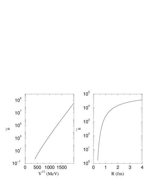
FIG. 7.: The average number of particles produced as a function of the depth of the potential field $\sqrt{V}$ is shown in the left panel, the size $R$ was fixed at 1 fm. The right panel shows the number of particles produced as a function of size $R$ given a fixed depth $V=1$ GeV${}^{2}\,.$ The time length of the perturbation is set at $T=$1 fm/c.

Fig. 7 shows the average number of particles as a function of the well size, right panel, and depth of the perturbation, left panel. The average number of particles grows approximately exponentially with the potential depth (Fig. 7, left panel). This is simply related to the fact that in a deep well the ground state energy grows almost linearly with the depth having $\Omega\approx\sqrt{V}$. By making the potential wider the ground state approaches the bottom of the well, limiting $\Omega$ to a constant. This restrains the growth of particles shown on the right panel of Fig. 7. One should bear in mind that the conditions considered are quite extreme and were used here to emphasize the character of the condensate. Practically the time scale may be shorter and perturbation weaker, leading to a more pre-condensate picture with much fewer pions. The total energy available in a heavy ion reaction may provide a guideline to what the perturbation $\Pi$ is and the realistic number of mesons produced are.

As a final part of this analysis we consider non-condensate pion production, which may be the main mechanism in most practical situations. Eq. (78) with the additional help of Eq. (79) results in the following form for $s$-wave pions from the continuum

$$\overline{n}={2V^{2}\over\pi^{2}}\,\int_{0}^{\infty}d\kappa\,\int_{0}^{\infty}dk{\left(k\sin(\alpha R)\,\cos(kR)-\alpha\,\cos(\alpha R)\sin(kR)\right)^{2}\over(\alpha^{2}-k^{2})^{2}\omega_{k}W_{\kappa}\left(\omega_{k}+W_{\kappa}\right)^{2}}\,,$$ (81)

where parameter $\alpha$ is defined as $\alpha=\sqrt{\kappa^{2}+V}$, $W_{\kappa}=\sqrt{\kappa^{2}+m_{\pi}^{2}}\,,$ and $\omega_{k}=\sqrt{k^{2}+m_{\pi}^{2}}$ are the total energies of the corresponding modes. As expected, the number of particles produced with no condensate involved is quite small. The left panel in Fig. 8 shows the average number of non-condensate pions as a function of the potential depth for different spatial sizes $R=$0.5, 1, 2 fm. The right panel of the same figure displays the dependence on the size $R$ for various values of $V\,.$ The important conclusion here is that the number of non-condensate pions ranges from a few up to maybe a dozen for extreme cases. This number is completely negligible in the presence of a strong condensate that produces hundreds of mesons. However, present experiments may just barely reach the point of the phase transition, and therefore the fraction of non-condensate pions is considerable, if not dominant. Moreover, other (conventional) mechanisms of pion production have to be taken into account.

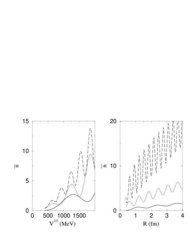
FIG. 8.: The left side shows the average number of pions of a particular type as a function of $V\,,$ the depth of the perturbation. Curves displayed as solid, dotted and dashed lines correspond to the values of the radius $R$ of 0.5, 1, and 2 fm, respectively. Plotted on the right hand side is the number of pions versus the radius $R$ for values of $\sqrt{V}$ of 0.5, 1 and 2 GeV as solid, dotted and dashed lines, respectively.

V Summary and conclusions

Our prime objective in this work was to study a mechanism of pion production in heavy ion collisions related to the creation of a chiral condensate and to explore how pion distributions can signal the presence of a condensate. We studied meson production by imposing a pion dispersion relation specific to the medium, i.e. with a space- and time-dependent effective mass.

In general, the problem of parametric excitation of the field quanta presents an interesting question as it is encountered in many branches of physics from condensed matter to high energy physics. The problem also exhibits a vast variety of solutions ranging from adiabatic to phase transitions and condensates.

We have conducted an extensive study of quantum field equations of a general form of Eq. (2). In our picture the parametric excitation of the field quanta is carried out by the externally given space- and time-dependent mass term. This term in the Lagrangian is quadratic in the field, and the states produced are often called “squeezed” [27, 28, 30, 31]. Some analogy can be drawn here from well studied linear current type terms that produce coherent states. However, the essential difference between coherent and squeezed states arises due to the fact that the latter correspond to the pairwise generation of quanta. In the case of pseudoscalar pions, this means that charge, isospin and parity are exactly preserved. We have emphasized the fact that the quantum solution can be built from the classical solution, and this important link was established via a canonical Bogoliubov transformation.

With our interest lying in the direction of chiral condensate we focused our attention on the potential of Eq. (2) to form a condensate with fast particle production and large correlations when the effective mass goes through zero. Along with a general formalism that can be used for numerical studies we have analytically solved the problem when the effective mass experiences sudden abrupt changes. Consideration of this particular temporal perturbation allowed us to clearly separate the exponentially rising collective pion condensate modes for any given spatial form of the perturbation in the effective mass. This produced conditions where the condensate and its signatures can be seen.

We have identified two basic channels of pion production. The first involves only a few discrete condensate modes and a large associated pion population. The second leads to the production of far fewer (non-condensate) particles with a broad phase space distribution. Mathematically these channels can be identified as production of mesons from bound and continuum states of a Schrödinger equation with a potential of the form of the perturbation itself, see Fig. 5. The bound states of negative energy are responsible for the characteristic features of the condensate.

Numerically, the number of non-condensed pions ranges from a few up to a dozen, and as expected is not very sensitive to the choice of the spatial and temporal form of the perturbation in the effective mass. In contrast, the condensate modes have an exponential sensitivity to the input parameters. As the abrupt changes in the effective pion mass grow in strength, a critical point is reached with the appearance of the condensate mode. The population of this mode increases dramatically from zero to thousands with a further slight change in the mass parameter. Due to this hyper-sensitivity of the number of condensed pions to the perturbation it is practically impossible to predict the effect quantitatively without specifying precisely the scenario of the process.

However, our results predict the number of non-condensate pions, thereby imposing a lower limit on the statistics needed to unambiguously detect the chiral condensate. Furthermore, we have shown that the condensate pions have a specific momentum distribution due to their common collective condensate mode. We have also shown that although the distribution over species starts from the famous $1/\sqrt{f}$ form for one mode it quickly becomes Gaussian with the appearance of successive modes. Therefore the presence of several modes complicates the detection of a chiral condensate. The number of modes present increases with energy. In addition, the mass parameter can be strongly perturbed in more than one region, each increasing the number of modes. Tunneling and chaotic dynamics in the resulting multi-well potential might lead to another class of interesting problems.

This work can be extended in several directions. With the formalism presented here, large numerical studies of the effective pionic field in a hot medium can be conducted involving realistic and even self-consistent forms of the perturbation given by the $\sigma$ field. Constraints on the perturbation of the mass parameter should be related more rigorously to observables. Further analysis of our results applied to phase transitions, zero mass particle production, energy transfer and many other field theory problems would definitely be fruitful. We feel that this work may provide a step forward in the study and classification of field theories with parametric excitations and possibly clarify the nature of the produced squeezed states.

REFERENCES

- [1] C. M. G. Lattes, Y. Fujimoto, and S. Hasegawa, Phys. Rep. 65 , 151 (1980).
- [2] A. A. Anselm, Phys. Lett. B 217, 169 (1989).
- [3] A. A. Anselm, JETP Lett. 59, 503 (1994).
- [4] J. D. Bjorken, K. L. Kowalski, and C. C. Taylor, SLAC Report No. SLAC-PUB-6109, 1992 (unpublished).
- [5] A. A. Anselm and M. G. Ryskin, Z. Phys. A 358, 353 (1997).
- [6] K. L. Kowalski, and C. C. Taylor, Case Western Reserve University Report No. CWRUTH-92-6, 1992 (unpublished).
- [7] S. Pratt and V. Zelevinsky, Phys. Rev. Lett. 72, 816 (1994).
- [8] Z. Huang and M. Suzuki, Phys. Rev. D 53, 891 (1996).
- [9] Z. Huang, I. Sarcevic, and R. Thews, Phys. Rev. D 54, 750 (1996).
- [10] J. Randrup and R. Thews, Phys. Rev. D 56, 4392 (1997).
- [11] Y. Kluger, F. Cooper, E. Mottola, J.P. Paz, and A. Kovner, Nucl. Phys. A 590, 581c (1995).
- [12] F. Cooper, Y. Kluger, E. Mottola, and J. P. Paz, Phys. Rev. D 51, 2377 (1995).
- [13] M. A. Lampert and J. F. Dawson, Phys. Rev. D 54, 2213 (1996).
- [14] M. Asakawa, Z. Huang, and X. Wang, Phys. Rev. Lett. 74, 3126 (1995).
- [15] G. Amelino-Camelia, J. D. Bjorken, and S. E. Larsson, Phys. Rev. D 56, 6942 (1997).
- [16] K. Rajagopal and F. Wilczek, Nucl. Phys. B 404, 577 (1993).
- [17] D. Horn and R. Silver, Annals of Physics 66, 509 (1971).
- [18] V. Koch, International Journal of Modern Phys. E, Vol 6, No 2, 203 (1997)
- [19] K. Rajagopal, Quark-Gluon Plasma 2, ed. R. Hwa (World Scientific, 1995).
- [20] E. Henley and W. Thirring, Elementary Quantum Field Theory (McGraw-Hill, 1962).
- [21] V. Popov and A. Perelomov, JETP 29, 738 (1969).
- [22] V. Popov and A. Perelomov, JETP 30, 910 (1970).
- [23] A. Baz, I. Zeldovich, and A. Perelomov, Scattering, Reactions and Decays in Nonrelativistic Quantum Mechanics (Nauka, Moscow 1971).
- [24] B. R. Mollow, Phys. Rev. 162, 1256 (1967).
- [25] J-P. Blaizot and G. Ripka, Quantum theory of finite systems (MIT Press, Cambridge, 1986).
- [26] R. J. Glauber, Phys. Rev. 131, 2766 (1963).
- [27] B. Picinbono and M. Rousseau, Phys. Rev. A1, 635 (1970).
- [28] W-M. Zhang, D. H. Feng, and R. Gilmore, Rev. Mod. Phys. 62, 867 (1990).
- [29] C. Eckart, Phys. Rev. 35, 1303 (1930).
- [30] F. DiFilippo, V. Natarajan, K. Boyce, and D. Pritchard, Phys. Rev. Lett. 68, 2859 (1992).
- [31] J. Aliaga, G. Crespo, and A. N. Proto, Phys. Rev. Lett. 70, 434 (1993).