THE CANONICAL NUCLEAR MANY-BODY PROBLEM AS A RIGOROUS EFFECTIVE THEORY

Abstract

The shell model is the standard tool for addressing the canonical nuclear many-body problem of nonrelativistic nucleons interacting through a static potential. We discuss several of the uncontrolled approximations that are made in this model to motivate a different approach, one based on an exact solution of the Bloch-Horowitz equation. We argue that the necessary self-consistent solutions of this equation can be obtained efficiently by a Green’s function expansion based on the Lanczos algorithm. The resulting effective theory is carried out for the simplest nuclei, d and ³He, using realistic NN interactions such as the Argonne $v18$ and Reid93 potentials, in order to contrast the results with the shell model. We discuss the wave function normalization, the evolution of the wave function as the “shell model” space is varied, and the magnetic elastic effective operator. The numerical results show a simple renormalization group behavior that differs from effective field theory treatments of the two- and three-body problems. The likely origin of this scaling is discussed.

1 Introduction

In many text books the shell model (SM) is motivated by the analogy with Brueckner’s treatment of nuclear matter. While the exact many-body Hamiltonian operates in an infinite Hilbert space

$$H={1\over 2}\sum_{i,j=1}^{A}(T_{ij}+V_{ij}),$$ (1)

where $T_{ij}$ is the relative nonrelativistic kinetic energy operator and $V_{ij}$ the nucleon-nucleon potential, the SM Hamiltonian acts in a restricted space and employs a softer “effective” potential,

$$H_{SM}={1\over 2}\sum_{i,j=1}^{A}(T_{ij}+V^{eff}_{ij}).$$ (2)

Motivating $H_{SM}$ is the notion that the determination of $V^{eff}$ might be simpler than solving the original A-body problem: the foundation of Brueckner theory is that high-momentum contributions to the wave function might be integrated out in a rapidly converging series in $\rho_{nuclear}$ or, equivalently, in the number of nucleons in high-momentum states interacting at one time outside the SM space.

The SM thus represents explicitly $\sim$ 60% of the wave function that resides at long-wavelengths, treating the A-body correlations important to collective modes by direct diagonalization. Implicitly the high-momentum components are swept into a rather poorly defined “effective interaction,” often determined empirically. The strength of the SM resides in the first of these two aspects: the technology developed for direct diagonalizations is quite remarkable, including recent progress in Lanczos-based methods [1], in treatments of light nuclei involving many shells [2], and in Monte Carlo sampling [3, 4]. Its weakness is the numerous uncontrolled approximations that become apparent when one tries to view the shell model as a faithful effective theory (ET). The thesis of this talk is that the same numerical strides that have advanced shell model diagonalizations now allow us to remove these uncontrolled approximations. The resulting ET has many differences with the shell model and many similarities to the effective field theories under discussion at this workshop.

Among the SM uncontrolled approximations are the following:
1) Even in lowest order, where only the pairwise interaction of high-momentum nucleons is included in $H^{eff}$, the functional form of the resulting effective interaction is not as simple as assumed in the SM,

$$\langle|H^{eff}|\rangle_{SM}\equiv\langle\alpha\beta|H^{eff}|\gamma\delta\rangle$$ (3)

where the Greek symbols label single-particle shell-model states. For example, if the Slater determinants are formed from harmonic oscillator states, the two-body matrix elements must carry an additional index labelling the total number of quanta in the configuration on which $H^{eff}$ operates [5]. Thus $H^{eff}$ reduces to the shell-model form only when that index is unnecessary, e.g., when a lowest-order calculation is restricted to a single shell. Beyond lowest order, three-, four-, and higher-body operators are successively added to $H^{eff}$.
2) Typically $H^{eff}$ lacks the symmetries of the original bare $H$, e.g., translational invariance and Hermiticity (though the latter is often enforced by hand).
3) SM wave functions are orthogonal and normed to unity. In ET the effective wave functions are naturally defined as the restrictions of the true wave functions $|\Psi_{i}\rangle$ to the model space

$$|\Psi_{i}\rangle\begin{array}[t]{c}\longrightarrow\\ ET\end{array}\langle SM|\Psi_{i}\rangle|SM\rangle\equiv|\Psi_{i}^{eff}\rangle.$$ (4)

Thus the norms are less than unity and orthogonality, which holds for the true wave functions, is lost when these wave functions are restricted to the model space.
4) Shell model interactions frequently depend on fictitious parameters such as “starting energies,” introduced to adjust the energy denominator in the two-body G-matrix or to account for intermediate-state average energies when the two-body G-matrix is iterated to produce some approximation to a higher order $H^{eff}$.
5) Perhaps most serious, the important issue of effective operators is almost never addressed in a meaningful way. In many cases practitioners adopted a phenomenological $H^{eff}$ which, while successful in producing spectra, provides no diagrammatic basis for calculating effective operators or wave function normalizations. Even in cases where $H^{eff}$ is derived from some underlying NN interaction, the practice is generally to then employ bare operators. In some well-studied cases, such as allowed $\beta$ decay in the $1p$ and $2s1d$ shells, it is then recognized that a phenomenological renormalization (e.g., $g_{A}\rightarrow$ 1) of operators greatly improves agreement with experiment. But the origin of this renormalization and its evolution with momentum transfer $q$ are left unclear. The situation is very unsatisfactory and undercuts the shell model as a predictive tool.

2 Self-consistent Bloch-Horowitz Solutions

We consider the cononical nuclear structure problem of nonrelativistic point nucleons interacting through a realistic NN interaction, such as the Argonne $v18$ [6] and Reid93 [7] potentials. The question is whether the uncontrolled approximations in the shell model can be removed, leaving a more complicated but still tractable effective theory. The approach involves three major steps:

$\bullet$ Formulating a treatment of effective interactions and operators that exploits the basic assumption in Brueckner theory — that interactions at high momenta can be integrated out in a cluster expansion (essentially an expansion in $\rho a^{3}$, where $\rho$ is the nuclear density and $a$ an interaction range) — but is otherwise exact. The convergence of the expansion could then be tested numerically and should depend on the operator under study and the momentum transfer. The goal would be to distinguish fully converged results from those which require higher order calculations.

$\bullet$ To find numerical tricks for implementing this formulation, demonstrating their validity in cases (e.g, A=2,3,4) where the expansion can be carried to all orders, so that the answers should then agree with Faddeev and other exact methods.

$\bullet$ To imbed the formulation in a heavier nucleus, where the cluster expansion can be carried out only partially.

There is some reason for optimism that if the first two goals can be achieved, the third might yield very accurate results: the Argonne group cluster variational Monte Carlo effort on ¹⁶O appeared to yield nearly exact results when clusters up to A = 5 were included. In this talk our efforts on the first two points will be described. In particular, we will be able to contrast an exact ET of the deuteron and ³He with the shell model to illustrate the shortcomings of the later: we think the differences are surprising.

The approach is sketched in Fig. 1. The Hilbert space is divided into a long-wavelength “shell model” space, defined by some energy scale $\Lambda_{SM}$, and a high-momentum space. One can truncate the latter at some scale $\Lambda_{\infty}\sim 3$ GeV, characteristic of the cores of realistic potentials, as above this energy, excitations make a negligible contribution. That is,

$$H^{eff}_{(i)}(\Lambda_{SM},\Lambda_{\infty})\begin{array}[t]{c}\longrightarrow\\ \Lambda_{\infty}\mathrm{~{}large}\end{array}H^{eff}_{(i)}(\Lambda_{SM}).$$ (5)

All correlations within the “SM” space are included, but the high-momentum correlations in the excluded space are limited to n-body, where n is the cluster size. Thus the lowest order effective interaction is

$$H^{eff}_{(n=2)}\equiv H^{eff}_{(n=2,0)}$$ (6)

It corresponds to embedding the A-body ladder diagram of Fig. 1b between SM states: A-2 of the nucleons are spectators, with the remaining pair scattering via a two-body ladder. The notation (n=2,0) states that the two-body cluster has no explicit dependence on the nuclear density, varying as $\rho^{0}$. The n=3 A-body ladder of Fig. 1c is similarly

$$H^{eff}_{(n=3)}\equiv H^{eff}_{(n=2,1)}+H^{eff}_{(n=3,0)}$$ (7)

where $H^{eff}(n=2,1)$ is the two-body part of the three-body ladder

$$\langle\alpha\beta|H^{eff}_{(n=2,1)}|\alpha^{\prime}\beta^{\prime}\rangle=\sum_{\gamma\leq k_{F}}\langle\alpha\beta\gamma|H^{eff}_{(n=3)}|\alpha^{\prime}\beta^{\prime}\gamma-\alpha^{\prime}\gamma\beta^{\prime}+...\rangle,$$ (8)

where $k_{F}$ denotes the Fermi level. This decomposition – which is done only to emphasize the content of the cluster expansion – illustrates that $H^{eff}_{(n=3)}$ contains $H^{eff}_{(n=2,0)}$ as well as a correction to the two-body interaction that depends linearly on the density and is obtained by identifying one ingoing SM single-particle leg of the three-body ladder with one outgoing leg, summed over all occupied states. It also contains a true three-body piece $H^{eff}_{(n=3,0)}$, where three SM ingoing single-particle states connect to three distinct outgoing states after undergoing a series of scatterings outside the SM space. The point is simple pedagogy: treatments of successively larger clusters in the high-momentum space correct the lowest-order two-body $H^{eff}_{(n=2,0)}$ by adding terms proportional to the $\rho$, $\rho^{2}$, etc., in the spirit of Brueckner theory. It also adds true three-body terms, true four-body terms, etc. Thus an expansion through four-body clusters yields $H^{eff}_{(n=2,2)}$, the two-body interaction corrected through order $\rho^{2}$, $H^{eff}_{(n=3,1)}$, the three-body interaction through order $\rho$, and $H^{eff}_{(n=4,0)}$, a density-independent true four-body interaction.

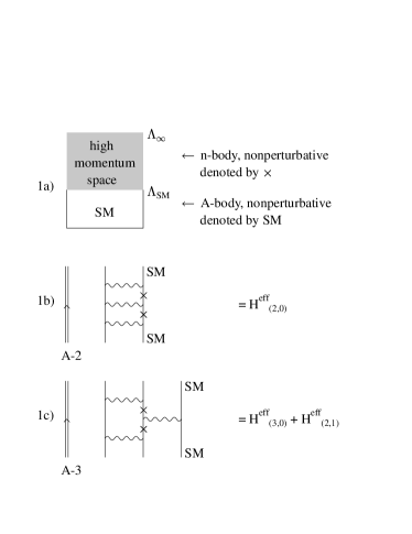
Figure 1: Cluster expansion of the effective interaction.

The calculation begins with a definition of the “SM” space. The goals of handling bound states and of generating an effective interaction that is translationally invariant leaves one sensible choice, many-body states constructed from harmonic oscillator Slater determinants. To exploit the relative/center-of-mass separability of harmonic oscillator Slater determinants, one must separate the SM and high-momentum spaces so that all configurations satisfying

$$E\leq\Lambda_{SM}\hbar\omega$$ (9)

are retained in the former. For example, a SM calculation of ¹⁶O with $\Lambda_{SM}=4+\Lambda_{0}$, where $\Lambda_{0}$ is the number of quanta in the ¹⁶O closed shell, would include all $4\hbar\omega$ configurations, e.g., $0p0h$, $2p2h$, and $4p4h$ excitations of nucleons from the $1p$ shell into the $2s1d$ shell, $1p1h$ excitations of a $1s$ shell nucleon into the $3s2d1g$ shell, etc. One can define the projection operator onto the high-momentum space by

$$Q_{SM}=Q(\Lambda_{SM},b).$$ (10)

where $b$ is the oscillator parameter. Thus the included or “SM” space is defined by two parameters, $\Lambda_{SM}$ and $b$. The preservation of translational invariance is also important numerically, as it reduces the two-body ladder to an effective one-body problem, etc.

The resulting Bloch-Horowitz equation [8] is then

$$H^{eff} = H+H{1\over E-Q_{SM}H}Q_{SM}H$$

$$H^{eff}|\Psi_{SM}\rangle = E|\Psi_{SM}\rangle~{}~{}~{}|\Psi_{SM}\rangle=(1-Q_{SM})|\Psi\rangle$$ (11)

where $|\Psi\rangle$ is the exact wave function and $H|\Psi\rangle=E|\Psi\rangle$. The difficulty posed by this equation is the appearance of the unknown energy eigenvalue in the equation for $H^{eff}$. Thus this system must be solved self-consistently. Note that there is no explicit reference to the harmonic oscillator in this equation: it enters only implicitly through $Q_{SM}$ in distinguishing the long-wavelength “SM” space from the remainder of the Hilbert space.

There is an extensive literature on this and similar equations, often involving a division of $H$ into an unperturbed $H_{0}$ and a perturbation $H_{1}=H-H_{0}$ [9, 10]. There are well-known pathologies with this division involving the effects of near-by intruder states on the perturbation expansion [11]. Here we explore another approach that is nonperturbative and involves, in effect, a computer summation of diagrams. The method is based on the Lanczos algorithm and offers a remarkably simple solution to the issue of self-consistency.

In the Lanczos algorithm a basis for representing a Hamiltonian is formed recursively in such a way that the resulting Hamiltonian is tridiagonal. Given a Hermitian operator $H$ and and an initial normalized vector $|v_{1}\rangle$, the successive steps are

$$H|v_{1}\rangle = \alpha_{1}|v_{1}\rangle+\beta_{1}|v_{2}\rangle$$

$$H|v_{2}\rangle = \beta_{1}|v_{1}\rangle+\alpha_{2}|v_{2}\rangle+\beta_{2}|v_{3}\rangle$$

$$H|v_{3}\rangle = ~{}~{}~{}~{}~{}~{}~{}~{}~{}~{}~{}\beta_{2}|v_{2}\rangle+\alpha_{3}|v_{3}\rangle+\beta_{3}|v_{4}\rangle~{}~{}etc.$$ (12)

so that the $H$ takes the form

$$H\rightarrow\left(\begin{array}[]{cccc}\alpha_{1}&\beta_{1}&0&\cdots\\ \beta_{1}&\alpha_{2}&\beta_{2}&\cdots\\ 0&\beta_{2}&\alpha_{3}&\cdots\\ \vdots&\vdots&\vdots&\end{array}\right)\left(\begin{array}[]{c}|v_{1}\rangle\\ |v_{2}\rangle\\ |v_{3}\rangle\\ \vdots\end{array}\right)$$ (13)

The remarkable property of this algorithm has to do with truncating the process in Eq. (12) after $n$ steps, where $n$ can be much smaller than the dimension of the Hilbert space. The resulting truncated matrix in Eq. (13) then contains the information needed to reconstruct the exact 2$n$-1 lowest moments of H over the eigenspectrum. As extremum eigenvalues are crucial to higher moments, one common application of the Lanczos algorithm is in determining such eigenvalues and their associated eigenfunctions. Another is to begin with the vector $|v_{1}\rangle=\hat{O}|g.s.\rangle$ and then use the algorithm to calculate the moments of the response of the ground state $|g.s.\rangle$ to the operator $\hat{O}$. A small number of moments, e.g., $\sim$ 100, often is sufficient to construct a response function with a numerical resolution comparable to that achieved experimentally.

A third application [12] is in constructing fully interacting Green’s functions. One finds

$${1\over E-H}|v_{1}\rangle=g_{1}(E)|v_{1}\rangle+g_{2}(E)|v_{2}\rangle+\cdots$$ (14)

where the $g_{i}(E)$ are continued fractions that depend on ${\alpha_{i},\beta_{i}}$ and where E appears only as a parameter. For example,

$$g_{1}(E)={1\over{E-\alpha_{1}-{\beta_{1}^{2}\over E-\alpha_{2}-{\beta_{2}^{2}\over E-\alpha_{3}-\beta_{3}^{2}}\cdots}}}$$ (15)

It follows that the Bloch-Horowitz equation can be solved self-consistently with only a single solution of the effective interactions problem, even in cases where multiple bound states are needed. The procedure is:

$\bullet$ For each relative-coordinate vector in the SM space $|\gamma\rangle$, form the excluded-space vector $|v_{1}\rangle\equiv Q_{SM}H|\gamma\rangle$ and the corresponding Lanczos matrix for the operator $Q_{SM}H$. Retaining the resulting coefficients ${\alpha_{i},\beta_{i}}$ for later use, construct the Green’s function for some initial guess for $E$ and then the dot product with $\langle\gamma^{\prime}|H$ to find $\langle\gamma^{\prime}|H^{eff}(E)|\gamma\rangle$.

$\bullet$ Perform the “SM” calculation to find the desired eigenvalue $E^{\prime}$ which, in general, will be different from the guess $E$. Using the stored ${\alpha_{i},\beta_{i}}$, recalculate the Green’s function for $E^{\prime}$ and $H^{eff}(E^{\prime})$ then redo the “SM” calculation. Repeat until convergence, i.e., until the input $E^{\prime}$ in the Green’s function equals the desired output “SM” eigenvalue.

$\bullet$ Then proceed to the next desired bound state, e.g., the first excited state, and repeat the above step. Note that it is not necessary to repeat the $H^{eff}$ calculation. The eigenvalue taken from the “SM” calculation is, of course, that of the first excited state. The procedure then generates distinct $H^{eff}(E^{\prime})$s for each desired state.

The attractiveness of this approach is that the effective interactions part of the procedure, which is relatively time consuming as it requires one to perform a large-basis Lanczos calculation for each relative-coordinate starting vector in the “SM” space, is performed only once. The diagonalization in the model space is generally much faster: modern workstations can handle even large-dimension shell model calculations (sparse matrices of $d\sim 10^{6}$) quickly ($\sim$ 30 minutes). In practice we found that self-consistency is achieved easily: six to eight cycles is typical. (More cycles are required for states with small binding energies.) Thus it is quite practical to derive the exact $H^{eff}(E)$s for a series of bound states.

Now we discuss the results of applying this procedure to the simplest nuclei, d and ³He, carrying the above process to completion (two-body and three-body ladders, respectively). The motivation is two-fold: demonstrate the numerical procedures we described above, and provide for the first time exact effective theory results that can be compared to those of the shell model.

The harmonic oscillator mode expansion must be sufficient to represent both the long-distance tails of bound states and the short-distance “hard core” scattering predicted by realistic NN potentials. (The Argonne v18 ${}^{1}S_{0}$ potentials are shown in Fig. 2.) Inclusion of high-momentum states through $\Lambda_{\infty}\sim 50$ yields a deuteron binding energy accurate to $\sim$ 60 keV; extending this to $\sim$ 140 produces a result accurate to one keV, provided one chooses an oscillator parameter that optimizes the convergence. (However, as we will discuss in Section 3, there appears to be a simple scaling with $\Lambda_{\infty}$ that allows one to extrapolate results to $\Lambda_{\infty}\rightarrow\infty$. When this is done, the small binding energy differences that result at $\Lambda_{\infty}=140$ for a reasonable choices of $b$ all but disappear. We will return to this point in Section 2.) Fig. 3 shows the rate of convergence as a function of $b$ and $\Lambda_{\infty}$. The rate of convergence for ³He is similar to that for the deuteron: a $\sim$ 60 keV energy accuracy is achieved at a $\Lambda_{\infty}$ of $\sim$ 50.

Figure 2: The Argonne $v18$ ${}^{1}S_{0}$ potentials.

The binding energies and operator matrix elements for simple systems like ³He can, of course, be calculated by other methods, e.g., Faddeev techniques or Green’s function Monte Carlo. We thus want to stress that the point of the following discussion is to do analogous calculations in the context of an effective theory, so that we begin to see the shortcomings of conventional techniques like the shell model as well as possibilities for overcoming those shortcomings. A first test of the techniques outlined above is to solve the Bloch-Horowitz equation for some SM-like space to then see if the resulting self-consistent energy is, indeed, the correct value. For model spaces of 2, 4, 6, and 8$\hbar\omega$ in the case of the deuteron we obtained a binding energy of -2.224 MeV (using $\sqrt{2}b=1.6f$ and $\Lambda_{\infty}=140$). The exact result is -2.2246 MeV. Similar agreement was obtained for ³He.

Figure 3: Deuteron ground state energy convergence as a function of $\Lambda_{\infty}$ for several choices of the oscillator parameter $b$. This b is defined as in the independent-particle SM: the corresponding b for relative motion is $\sqrt{2}$ times the values shown. It is clear that if an inappropriate size is chosen for the basis states (e.g., b=1.9), the rate of convergence can be greatly slowed.

More interesting is the evolution of the wave functions, shown in Tables 1 and  2. Various ET calculations were done in small model spaces, analogous to shell model spaces, consisting of all 2$\hbar\omega$ configurations, all 4$\hbar\omega$ configurations, etc. For each such space we then solved the Bloch-Horowitz equation via the Lanczos Green’s function method described above, iterating the shell model calculation until the self-consistent energy is fully converged. The deuteron and ³He calculations involve two- and three-body ladder sums in the excluded space, yielding sets of two- and three-body “SM” matrix elements of $H^{eff}$ for the model spaces. The deuteron calculation is rather trivial; for $\Lambda_{\infty}\sim 50$ the ³He BH calculation involves a dense matrix of dimension $\sim 10^{4}$, still rather modest by current SM standards. The matrix is dense because we work in relative Jacobi coordinates, rather than an m-scheme, utilizing standard Talmi-Brody-Moshinshy methods [13]. (See Ref. [14] for details.) The results in Table 2 were obtained with approximately 100 Lanczos iterations: it is apparent that the convergence is then quite good. The wave functions must be normalized according to Eq. (11): this involves calculating unity as an effective operator. We will return to this point below.

Table 1: ET results for the deuteron ground state wave function calculated with the Argonne $v18$ potential. The columns on the right correspond to different choices of the ET model space, the analog of a SM space. The rows correspond to the resulting amplitudes for the designated, selected configurations $\mid n,{}^{S}L_{J}\rangle$. The quantities within the parentheses are the square of the norm of the effective wave function, e.g., the probability that the deuteron resides in the corresponding “SM” space.

	amplitude
basis state	0$\hbar\omega$	2$\hbar\omega$	4$\hbar\omega$	6$\hbar\omega$	8 $\hbar\omega$	exact
	(65.9%)	(79.5%)	(86.1%)	(91.3%)	(93.0%)	(100%)
$\mid$ 1, ${}^{3}S_{1}\rangle$	0.81155	0.81154	0.81155	0.81155	0.81152	0.81155
$\mid$ 2, ${}^{3}S_{1}\rangle$	0.00000	-0.31483	-0.31483	-0.31483	-0.31482	-0.31483
$\mid$ 1, ${}^{3}D_{1}\rangle$	0.00000	0.19524	0.19524	0.19524	0.19523	0.19524
$\mid$ 3, ${}^{3}S_{1}\rangle$	0.00000	0.00000	0.24945	0.24945	0.24944	0.24945
$\mid$ 4, ${}^{3}S_{1}\rangle$	0.00000	0.00000	0.00000	-0.20851	-0.20850	-0.20851
$\mid$ 5, ${}^{3}S_{1}\rangle$	0.00000	0.00000	0.00000	0.00000	0.12596	0.12596

The tables show the lovely evolution of the wave function in ET, an evolution quite unlike that of typical shell model calculations. The wave functions obtained in different model spaces agree over overlapping parts of their Hilbert spaces. Thus as one proceeds through 2$\hbar\omega$, 4$\hbar\omega$, 6$\hbar\omega$, … calculations, the ET wave function evolves only by adding new components in the expanded space. The normalization of the wave function grows accordingly. Thus, for ³He, the 0$\hbar\omega$ ET calculation contains 0.311 of the full wave function in the effective space; the 0+2+4$\hbar\omega$ result is 0.700.

This evolution will not arise in the standard SM because the wave function normalization is set to unity regardless of the model space. It will also not arise for a second reason, illustrated in Table 3. The matrix elements of $H^{eff}$ are crucially dependent on the model space: the listed results for ³He show that a typical matrix $\langle\alpha|H^{eff}|\beta\rangle$ changes very rapidly under modest expansions of the model space, e.g., from 2$\hbar\omega$ to 4$\hbar\omega$. Yet it is common practice in the shell model to expand calculations by simply adding to an existing SM Hamiltonian new interactions that will mix in additional shells. We suspect the behavior found for ³He is generic in ET calculations: it arises because a substantial fraction of the wave function lies near but outside the model space (e.g., see Table 2). An expansion of the model space changes the energy denominators for coupling to some of these configurations, and moves other nearby configurations from the excluded space to the model space. Naively, relative changes in effective interaction matrix elements of unity are expected.

Table 2: As in Table 1, only for ³He. The basis states are now designated somewhat schematically as $\mid N,\alpha\rangle$, where $N$ is the total number of oscillator quanta and $\alpha$ is an index representing all other quantum numbers.

	amplitude
state	0$\hbar\omega$	2$\hbar\omega$	4$\hbar\omega$	6$\hbar\omega$	8 $\hbar\omega$	exact
	(31.1%)	(57.4%)	(70.0%)	(79.8%)	(85.5%)	(100%)
$\mid 0,1\rangle$	0.55791	0.55791	0.55791	0.55795	0.55791	0.55793
$\mid 2,1\rangle$	0.00000	0.04631	0.04613	0.04618	0.04622	0.04631
$\mid 2,2\rangle$	0.00000	-0.48255	-0.48237	-0.48243	-0.48243	-0.48257
$\mid 2,3\rangle$	0.00000	0.00729	0.00731	0.00730	0.00729	0.00729
$\mid 2,4\rangle$	0.00000	0.16707	0.16698	0.16706	0.16706	0.16708
$\mid 2,5\rangle$	0.00000	0.00566	0.00564	0.00565	0.00565	0.00566
$\mid 2,6\rangle$	0.00000	-0.00017	-0.00017	-0.00017	-0.00017	-0.00017
$\mid 4,1\rangle$	0.00000	0.00000	-0.02040	-0.02042	-0.02043	-0.02047
$\mid 4,2\rangle$	0.00000	0.00000	0.11267	0.11274	0.11275	0.11289
$\mid 4,3\rangle$	0.00000	0.00000	-0.04191	-0.04199	-0.04208	-0.04228
$\mid 4,4\rangle$	0.00000	0.00000	0.28967	0.28978	0.28978	0.29001
$\mid 4,5\rangle$	0.00000	0.00000	0.01059	0.01059	0.01059	0.01059
$\mid 4,6\rangle$	0.00000	0.00000	-0.00213	-0.00212	-0.00211	-0.00210
$\mid 4,7\rangle$	0.00000	0.00000	0.00998	0.01000	0.01000	0.01000
$\mid 4,8\rangle$	0.00000	0.00000	-0.11319	-0.11327	-0.11330	-0.11335
$\mid 4,9\rangle$	0.00000	0.00000	0.08446	0.08447	0.08446	0.08448
$\mid 4,10\rangle$	0.00000	0.00000	-0.08613	-0.08626	-0.08632	-0.08638
$\mid 4,11\rangle$	0.00000	0.00000	-0.00210	-0.00211	-0.00211	-0.00211
$\mid 4,12\rangle$	0.00000	0.00000	-0.00252	-0.00254	-0.00256	-0.00257
$\mid 4,13\rangle$	0.00000	0.00000	-0.00020	-0.00020	-0.00020	-0.00020
$\mid 4,14\rangle$	0.00000	0.00000	-0.00010	-0.00010	-0.00010	-0.00010
$\mid 4,15\rangle$	0.00000	0.00000	-0.00012	-0.00013	-0.00012	-0.00012

Table 3: Selected BH 3-body effective interaction matrix elements for ³He, in MeV, illustrating the strong dependence on the “SM” space. The Argonne v18 potential was used.

	2$\hbar\omega$	4$\hbar\omega$	6$\hbar\omega$	8 $\hbar\omega$
$\langle 0,1\mid H^{eff}\mid 2,1\rangle$	-4.874	-3.165	-0.449	1.279
$\langle 0,1\mid H^{eff}\mid 2,5\rangle$	-0.897	-1.590	-1.893	-2.208
$\langle 2,1\mid H^{eff}\mid 2,2\rangle$	6.548	-2.534	-4.144	-5.060

Now we turn to the question of operators. The standard procedure in the SM is to calculate nuclear form factors with bare operators, or perhaps with bare operators renormalized according to effective charges determined phenomenologically at $q^{2}$ = 0, using SM wave functions normed to 1. As we now have a series of exact effective interactions corresponding to different model spaces, we can test the validity of this approach. The results for the elastic magnetic form factors for the deuteron and ³He are shown in Figs. 4 and 5. One sees in each case that by the time one reaches a momentum transfer $q\sim 2.5/f$, random numbers are being generated: bare operators used in conjunction with exact effective wave functions generate results that differ by an order of magnitude, depending on the choice of the model space. This is not surprising, of course. If one considers the operation

$$e^{i\vec{q}\cdot\vec{r}}\sigma\tau_{3}|g.s.\rangle$$ (16)

at momentum transfers $\mathrel{\hbox to0.0pt{\lower 4.0pt\hbox{\hskip 1.0pt$\sim$}\hss}\raise 1.0pt\hbox{$>$}}2k_{F}$, where $k_{F}$ is the Fermi momentum, most of the resulting amplitude should reside outside the long-wavelength model space, in any simple view of the nucleus. That is, the strength resides entirely in the effective contributions to the operator. If these components are ignored, the results have to be in error.

Figure 4: The magnetic elastic form factor for the deuteron calculated with the exact $H^{eff}$, SM wave functions normalized to unity, and a bare operator are compared to the exact result (solid line). When effective operators and the proper wave function normalizations are used, all results become identical to the solid line.

Clearly the effective interaction and effective operator have to be treated consistently and on the same footing. If $\hat{O}$ is the bare operator, one finds

$$\langle\Psi_{f}|\hat{O}|\Psi_{i}\rangle\equiv\langle\Psi_{f}^{eff}|\hat{O}^{eff}|\Psi_{i}^{eff}\rangle$$ (17)

where

$$\hat{O}^{eff}=(1+HQ_{SM}{1\over E_{f}-HQ_{SM}})\hat{O}(1+{1\over E_{i}-Q_{SM}H}Q_{SM}H)$$ (18)

and where the effective wave function normalization of $|\Psi_{i}^{eff}\rangle$ and $|\Psi_{f}^{eff}\rangle$, mentioned earlier, must be determined using the effective operator $\hat{1}$, e.g.,

$$1=\langle\Psi_{i}|\Psi_{i}\rangle=\langle\Psi_{i}^{eff}|(1+HQ_{SM}{1\over E_{i}-HQ_{SM}})(1+{1\over E_{i}-Q_{SM}H}Q_{SM}H)|\Psi_{i}^{eff}\rangle$$ (19)

These expressions can be evaluated with the Lanczos Green’s function methods described earlier. When this is done, all of the effective calculations, regardless of the choice of the model space, yield the same result, given by the solid lines in Figs. 4 and 5.

Figure 5: As in Fig. 4, only for ${}^{3}He$.

We would argue, based on this example, that many persistent problems in nuclear physics — ranging from the renormalization of $g_{A}$ in $\beta$ decay [15] to the systematic differences between measured and calculated M1 form factors at Bates [16] — very likely are due to our naive treatments of operators. It should be apparent from the above example that no amount of work on $H^{eff}$ will help with this problem. What is necessary is a diagrammatic basis for generating $H^{eff}$ that can be applied in exactly the same way to evolving $\hat{O}^{eff}$. From this perspective, phenomenological derivations of $H^{eff}$ by fitting binding energies and other static properties of nuclei are not terribly helpful, unless one intends to simultaneously find phenomenological renormalizations for each desired operator in each $q^{2}$ range of interest.

3 Numerical Renormalization Group Speculations

While the Lanczos Green’s function method is reasonably elegant, the calculations described above have a “brute force” aspect in that the high-momentum ladders must be summed to very large $\Lambda_{\infty}$. In the of the deuteron we carried the sums to $\Lambda_{\infty}=140$ to assure one keV accuracy. The calculation for ³He was stopped at $\Lambda_{\infty}=52$, with a resulting binding energy of -6.842 MeV. As our calculations are otherwise exact, this is an upper bound: a variational principle operates as $\Lambda_{\infty}$ is increased. The corresponding Green’s function Monte Carlo result is -6.87 $\pm$ 0.03 MeV; Faddeev results for the v18 potential give -6.895 $\pm$ 0.001 MeV.

The ³He calculations can (and will) be carried further: the existing matrices are only of dimension 12000. However, there are alternatives to the brute-force approach. One rather simple idea is to evaluate, instead of the three-body ladder, the difference of the three-body ladder and the appropriate sum over the three corresponding two-body ladders, evolving this difference with $\Lambda_{\infty}$. The resulting $H^{eff}$ then would be obtained by adding to this difference the two-body ladder. While this is a tautology, our expectation is that the difference will converge more quickly than the full 3-body ladder as a function of $\Lambda_{\infty}$, since the difference would start with all pair wave functions being properly correlated. If one were able to truncate the 3-body difference calculation at a lower $\Lambda_{\infty}$ than the corresponding 2-body ladders, considerable efficiency would be gained. This possibility will soon be studied.

Another possibility has to do with an observation about the way both ground-state energies and matrix elements of $H^{eff}$ evolve with $\Lambda_{\infty}$. Our calculations are based on the division of the Hilbert space into two sectors

$$0\leq\Lambda\leq\Lambda_{SM}~{}~{}~{}~{}\Lambda_{SM}<\Lambda\leq\Lambda_{\infty}$$ (20)

While the deuterium calculation was done with a large value of $\Lambda_{\infty}$, we can bring it to a much lower value in order to study the evolution with $\Lambda_{\infty}$ (see Fig. 3). When the numerical results were examined, it was found that they scaled with $\Lambda_{\infty}$ simply, approximately as an exponential in $\Lambda_{\infty}^{2}$. For example, calculations were done for the Argonne $v18$ potential and $b$ = 1.7f, with $\Lambda_{\infty}$ = 46, 50, and 54, to which we fit the three-parameter functional form

$$E_{g.s.}(\Lambda_{\infty})=-2.175\mathrm{MeV}+3.178\mathrm{MeV}e^{-1.055(\Lambda_{\infty}/50)^{2}}$$ (21)

Thus -2.175 MeV is identified as the binding energy for $\Lambda_{\infty}\rightarrow\infty$, if this numerical renormalization group equation were exact. The deuteron binding energy at $\Lambda_{\infty}\sim 50$ is off by more than an MeV. Table 4 shows that 95% of this difference can indeed be anticipated by examining the running of the results for $\Lambda_{\infty}\sim 50$: the projected valued at $\Lambda_{\infty}=140$ is correct to $\sim$ 30 keV. For $b=1.13f$, the case converging most quickly in Fig. 3, a similar 30 keV accuracy is achieved for an extrapolation from still lower $\Lambda_{\infty}$, 34-40. Numerically, such an extrapolation can be done quite efficiently: with proper coding, it costs relatively little “overhead” to obtain additional results in the neighborhood of some starting $\Lambda_{\infty}$.

Table 4: A “numerical renormalization group” study of the running of the deuteron binding energy with $\Lambda_{\infty}$. The results in the middle column are exact. Those in the right column were obtained from Eq. (21), determined from the variation of the $E_{g.s.}(\Lambda_{\infty})$ near $\Lambda_{\infty}=50$. An oscillator parameter is $b=1.7f$, chosen so that this is a slowly converging case requiring significant extrapolation. The potential used is Argonne $v18$.

$\Lambda_{\infty}$	$E_{g.s.}^{calculated}$ (MeV)	$E_{g.s.}^{projected}$ (MeV)
46	-0.874	fit
50	-1.069	fit
54	-1.247	fit
60	-1.476	-1.480
70	-1.771	-1.773
80	-1.961	-1.962
90	-2.077	-2.071
100	-2.143	-2.128
110	-2.179	-2.156
120	-2.196	-2.167
130	-2.204	-2.172
140	-2.207	-2.174

The corresponding exercise was done for ³He using results for $\Lambda_{\infty}$ = 44, 48, and 52. A very similar functional form is found

$$E_{g.s.}(\Lambda_{\infty})=-6.906\mathrm{MeV}+0.403\mathrm{MeV}e^{-1.57(\Lambda_{\infty}/48)^{2}}$$ (22)

While we do not have exact results similar to those in Table 4, the resulting asymptotic value of -6.906 MeV is in good agreement with the Faddeev value of 6.895 $\pm$ 0.001 MeV. Such 10 keV accuracy compares well with the Green’s function Monte Carlo result, with its 30 keV accuracy.

Now all of this poses an interesting question: our “renomalization group” evolution is a nontrivial one, as it involves a truncation in harmonic oscillator energies for few-body Slater determinants. Yet it appears this truncation is leading to a very simple exponential convergence in results. This can be compared to effective field theory, where the truncation is made on the range of the potential and the convergence is a weaker 1/$\Lambda_{\infty}$. Can one derive and therefore understand this attractive aspect of a harmonic oscillator mode expansion for bound states?

To attack this problem, we envision setting $\Lambda_{\infty}$ to some intermediate scale $\sim$ 50 (around 750 MeV) — similar to the numerical examples above — and performing, prior to our SM effective theory, a preliminary integration over modes above this scale. If we write

$$H\equiv H_{0}+H^{\prime}~{}~{}~{}~{}~{}\mathrm{and}~{}~{}~{}~{}~{}H^{eff}=H_{0}+H^{\prime eff}$$ (23)

where $H_{0}$ is the harmonic oscillator Hamiltonian and $H^{eff}$ is the appropriate effective interaction to use below $\Lambda_{\infty}$, then we find

$$H^{\prime eff}=H^{\prime}+H^{\prime}G^{0}_{\Lambda_{\infty}}H^{\prime eff}$$ (24)

where $G^{0}_{\Lambda_{\infty}}$ is the harmonic oscillator Green’s function corresponding to high-momentum scattering, e.g.,

$$G^{0}_{\Lambda_{\infty}}(\vec{r}_{1},\vec{r}_{2}) = \sum_{\Lambda>\Lambda_{\infty}}{|\Psi^{HO}_{\Lambda}(\vec{r}_{1})\rangle\langle\Psi^{HO}_{\Lambda}(\vec{r}_{2})|\over E-E_{\Lambda}}$$ (25)

$$= G^{0}(\vec{r}_{1},\vec{r}_{2})-\sum_{\Lambda\leq\Lambda_{\infty}}{|\Psi^{HO}_{\Lambda}(\vec{r}_{1})\rangle\langle\Psi^{HO}_{\Lambda}(\vec{r}_{2})|\over E-E_{\Lambda}}$$

In Eq. (24) the high-momentum ladder sum involves terms of the form

$$\Psi^{f*}_{SM}(\vec{r}_{1})H^{\prime}(\vec{r}_{1})G^{0}_{\Lambda_{\infty}}(\vec{r}_{1},\vec{r}_{2})H^{\prime}(\vec{r}_{2})\Psi^{i}_{SM}(\vec{r}_{2})$$ (26)

The harmonic oscillator Green’s function has the attractive property that it can be decomposed as

$$G^{0}_{\Lambda_{\infty}}=G^{0}_{\Lambda_{\infty}}(r_{+},r_{-})$$ (27)

where $r_{+}=|\vec{r}_{1}+\vec{r}_{2}|$ and $r_{-}=|\vec{r}_{1}-\vec{r}_{2}|$. Now the restriction to large $\Lambda$ corresponds to short times and thus to short propagation distances. Thus propagation lengths should shorten as $\Lambda_{\infty}$ is increased. Furthermore the overall behavior of the Green’s function is governed by the factor $e^{-r_{+}r_{-}}$. Thus the propagator is most contracted along the $smaller$ of these two coordinates, $r_{<}=min(r_{+},r_{-})$. As the ladder will be evaluated between long-wavelength SM states, these observations suggest expanding $\Psi^{f*}_{SM}(\vec{r}_{1})H^{\prime}(\vec{r}_{1})$ and $H^{\prime}(\vec{r}_{2})\Psi^{i}_{SM}(\vec{r}_{2})$ in Eq. (26) around $r_{>}$ in a Taylor series in $r_{<}$. (There is a more pedagogical discussion of this technique and its relevance to effective field theory in Ref. [17].)

Figure 6: Contraction of a ladder diagram involving only very high momentum excluded states to a local operator.

After a bit of algebra, the net result is the contraction of the ladder sum to a local “rainbow” diagram, as illustrated in Fig. 6. The contracted Green’s function has a form familiar to most effective field theorists,

$$G_{\Lambda_{\infty}}\rightarrow g^{0}(r_{>})+\vec{\nabla}_{r_{>}}g^{2}(r_{>})\vec{\nabla}_{r_{>}}+...$$ (28)

where this is to be inserted between wave functions evaluated at $r_{>}$. The function $g^{0}(r_{>})$ is obtained by integrating $G_{\Lambda_{\infty}}(r_{+},r_{-})$ over $r_{<}$, while $g^{2}(r_{>})$ involves a second moment in the small coordinate $r_{<}$, etc. Effectively this sums the ladder according to a local density approximation ($g^{0}$), in an approximation that also takes into account the gradient of the local density ($g^{2}$), etc.

One of the most attractive features of the harmonic oscillator is that the full Green’s function was recently derived in closed form [18], so that $g^{0}(r_{>})$ can be calculated by integrating the last expression in Eq. (25): an infinite sum over high-momentum modes can be replaced by a finite sum over low-momentum modes. The full Green’s function is shown in Fig. 7, and the integration that produces $g^{0}$ is depicted in Fig. 8. The resulting $g^{0}$ for $\Lambda_{\infty}$ = 30 and 50 are shown in Figs. 9 and 10 (dashed lines) along with a similar contraction of the full Green’s function $G^{0}$. One finds that the dashed lines – the residual contribution of very high momentum excitations – rapidly oscillates, with a frequency very close to $\Lambda_{\infty}$. Thus a harmonic oscillator expansion converges not because every point in coordinate space is well represented by the included states, but because integration of a product of such oscillations with a smooth Hamiltonian yields a small remainder. Note that increasing $\Lambda_{\infty}$ also extends the range in $r_{>}$ spanned by the harmonic oscillator basis functions: extended wave functions require more work.

Figure 7: The full (summed over all modes) harmonic oscillator Green’s function. For parity conserving interactions, only the even or odd projections are needed. The even projection is shown.

We are now in the process of implementing this local approximation to see how far the integration scale $\Lambda_{\infty}$ can be lowered without loss of accuracy. Unlike effective field theory treatments, our Taylor series expansion involves a known potential and can be carried out term by term until exhaustion sets in. The results may provide some estimate of the scales that effective field theories need to reach to become very accurate.

Figure 8: The integration path in the $(r_{+},r_{-})$ plane that is used to contract $G(r_{+},r_{-})$ to $g_{0}(r_{>})$.

We will close with two speculations. If one folds the dashed-line functions of Figs. 9 and 10 with the potential of Fig. 2, the result is not dissimilar to a $j_{0}(\Lambda r_{>})$. Such a function, integrated with a product of harmonic oscillator wave functions, yields a factor $e^{-a\Lambda^{2}}$. Thus we are hopeful that this line of work may indeed explain the numerical scaling we have previously discussed. Our goal is to add to Table 4 a fourth column in which our phenomenological scaling function is replaced by a derived one that yields improved results: the “break” seen in Table 4 at $\Lambda_{\infty}\sim$ 100 (a scale characteristic of the Argonne $v18$ hard core) suggests there is a bit of physics missing from our phenomenological function. Second, this suggests that the rapid convergence of the harmonic oscillator mode expansion, as compared to effective field theory scaling of 1/$\Lambda_{\infty}$ which results from absorbing short-range contributions to the NN potential into contact terms, may be because it offers a better compromise between coordinate and momentum space. Hopefully we will be able to be more specific soon.

Figure 9: The dashed line is the $g_{0}(r_{>})$ that results when excitations $\Lambda>30$ are summed. The solid line is the corresponding result for the full Green’s function. It is the rapid oscillation of the dashed residual – rather than the accuracy of the harmonic oscillator expansion at all values of $r_{>}$ – that is responsible for the convergence. The oscillations are very regular and quite close in frequency to $\Lambda\sim 30$.

Figure 10: As in Fig. 9, only for $\Lambda>50$.

4 Outlook and Future Plans

The ability to efficiently solve ³He as an effective theory in a SM-like space is, in itself, quite significant: this means it is relatively straightforward to execute a faithful BH treatment of heavier nuclei through order $\rho$ in both the effective interaction and effective operators. The numerical effort is comparable.

The example of ³He also suggested that many of the uncontrolled approximations made in the SM cannot be justified. Recently sophisticated numerical advances have been made in SM calculations. We have argued that it may be equally important to train this numerical power on the shakey foundations of that model. A specific example is our use of the Lanczos algorithm – a favorite among SM practitioners – to generate the Green’s function, leading to a tractable strategy for solving the BH equation self-consistently.

We believe that, if the program in Section 3 has modest success, we should be able to handle ⁴He with an accuracy similar to that achieved already for ³He. That would imply that it is now possible to handle effective interactions and operators in finite nuclei through order $\rho^{2}$. At that point the exciting challenge will be to determine where convergence in the cluster expansion is being approached.

We would like to think that the work reported here will form a bridge between the ideas growing out of effective field theories, and the successful phenomenology we have achieved in traditional nuclear physics (particularly in modeling the NN potential and in solving few-body systems with nearly exact methods). It may also stimulate effective field theory, which has not yet had an impact on nuclear problems beyond NN and three-body systems. It is not inconceivable that a marriage of EFT – which strives to handle few-body problems rigorously, including relativity, fundamental few-body forces, etc. — with some kind of cluster expansion of the Brueckner type might someday yield a controlled theory of finite nuclei. Furthermore, the attractive exponential convergence of our harmonic oscillator mode expansion is also EFT “food for thought.”

This work was supported in part by the Division of Nuclear Physics, US Department of Energy.

References

References

- [1] E. Caurier, G. Martinez-Pinedo, F. Nowacki, A. Poves, J. Retamosa, and A. P. Zuker, Phys. Rev. C 59, 2033 (1999) and references therein.
- [2] P. Navratil and B. R. Barrett, Phys. Rev. C 57, 562 (1998) and Phys. Rev. C 59, 1906 (1999).
- [3] S. E. Koonin, D. J. Dean, and K. Langanke, Phys. Rep. 278, 1 (1997) and references therein.
- [4] T. Otsuka and T. Mizusaki, J. Phys. G 25, 699 (1999).
- [5] D. C. Zheng, B. R. Barrett, J. P. Vary, W. C. Haxton, and C.-L. Song, Phys. Rev. C 52, 2488 (1995).
- [6] R. B. Wiringa, V. G. J. Stoks, and R. Schiavilla, Phys. Rev. C 51, 38 (1995).
- [7] R. V. Reid, Jr., Ann. Phys. (N.Y.) 50, 411 (1968).
- [8] C. Bloch and J. Horowitz, Nucl. Phys. 8, 91 (1958).
- [9] B. R. Barrett and M. W. Kirson, in Advances in Nuclear Physics, ed. M. Baranger and E. Vogt, vol. 6 (Plenum, New York, 1973) p. 219.
- [10] T. T. S. Kuo and E. Osnes, Lecture Notes in Physics, ed. H. Araki et al., vol. 364 (Springer-Verlag, Berlin, 1990).
- [11] T. H. Shucan and H. A. Weidenmuller, Ann. Phys. (N.Y.) 73, 108 (1972) and 76, 483 (1973).
- [12] R. Haydock, J. Phys. A7, 2120 (1974).
- [13] M. Moshinsky, The Harmonic Oscillator in Modern Physics: From Atoms to Quarks (Gordon and Breach, New York, 1969).
- [14] C.-L. Song, An Improved Procedure for Calculating Effective Interactions and Operators, Univ. Washington Ph.D. thesis, 1998.
- [15] I. S. Towner, Phys. Rep. 155, 263 (1987); B. A. Brown, Nucl. Phys. A 522, 221c (1991); G. Martinez-Pinedo, A. Poves, E. Caurier, and A. P. Zuker, Phys. Rev. C 53, 2602 (1996).
- [16] R. S. Hicks et al., Phys. Rev. Lett. 60, 905 (1988) and references therein.
- [17] P. Lepage, How to Renormalize the Schroedinger Equation, nucl-th/9706029.
- [18] D. B. Khrebtukov and J. H. Macek, J. Phys. A 31, 2853 (1998).