KUNS 1579
Symmetry Breaking and Bifurcations in the Periodic Orbit Theory: I. Elliptic Billiard

Abstract

We derive an analytical trace formula for the level density of the two-dimensional elliptic billiard using an improved stationary phase method. The result is a continuous function of the deformation parameter (eccentricity) through all bifurcation points of the short diameter orbit and its repetitions, and possesses the correct limit of the circular billiard at zero eccentricity. Away from the circular limit and the bifurcations, it reduces to the usual (extended) Gutzwiller trace formula which for the leading-order families of periodic orbits is identical to the result of Berry and Tabor. We show that the circular disk limit of the diameter-orbit contribution is also reached through contributions from closed (periodic and non-periodic) orbits of hyperbolic type with an even number of reflections from the boundary. We obtain the Maslov indices depending on deformation and energy in terms of the phases of the complex error and Airy functions. We find enhancement of the amplitudes near the common bifurcation points of both short-diameter and hyperbolic orbits. The calculated semiclassical level densities and shell energies are in good agreement with the quantum mechanical ones.

1 Introduction

The periodic orbit theory (POT), developed by Gutzwiller [1, 2] for chaotic systems, by Balian and Bloch [3] for cavities, and by Berry and Tabor [4, 5] for integrable systems, has proved to be an important semiclassical tool not only for an approximate quantization, but also for the description of gross-shell effects in finite fermion systems [6, 7]. Gutzwiller’s approach has been extended to take into account continuous symmetries [6, 8, 9, 10, 11, 12] and is therefore applicable to systems with mixed classical dynamics, including the integrable and hard-chaos limits.

An important role is played by the classical degeneracy of the periodic orbits in systems with continuous spatial or dynamical symmetries: the orbits are then not isolated in phase space (as it was assumed in Gutzwiller’s original trace formula, and as is the case in chaotic systems), but occur in degenerate families with identical actions. The degree of degeneracy $\cal K$ is defined as the number of independent parameters which are necessary to uniquely specify an orbit within each family. E.g., the orbit families with the highest degeneracy in spherical systems with spatial $SO(3)$ symmetry have ${\cal K}=3$, corresponding to the three Euler angles that specify the orientation of an orbit within the plane of motion and the orientation of the plane itself; the orbit families in two-dimensional systems with $U(1)$ rotational symmetry have ${\cal K}=1$; the isotropic harmonic oscillator in 2 dimensions has $SU(2)$ symmetry and hence orbit families with ${\cal K}=2$. Orbits with different degeneracies $\cal K$ may also occur in one and the same system, such as the spherical cavity discussed by Balian and Bloch [3] where the diameter orbit has ${\cal K}=2$ and all other orbits have ${\cal K}=3$; the spheroidal cavity [13] where ${\cal K}=2$, 1 or 0 occurs (the latter corresponding to isolated orbits); or the elliptic billiard with ${\cal K}=1$ or 0, as discussed in the present paper.

However, problems arise for all these trace formulae in connection with the breaking of a continuous symmetry and with the bifurcation of stable periodic orbits when a continuous parameter (energy, deformation, external field) is varied. The reason is that at such critical points the standard stationary phase approximation, used for integrations in the derivation of the trace formula, breaks down and leads to divergences and/or discontinuities of the amplitudes in the trace formula. This happens most frequently in mixed systems, but it occurs also in integrable systems. Typical examples are the two-dimensional elliptic billiard and the three-dimensional spheroidal cavity. In the former, all repetitions of the short diameter orbits undergo bifurcations at specific deformations, whereby new families of hyperbolic orbits are created. Similarly in the latter system, the periodic orbits lying in the equatorial plane perpendicular to the symmetry axis bifurcate also at specific deformations, whereby new 3-dimensional orbits appear [13]. In both systems, all bifurcations and the limit to the spherical shape lead to divergent amplitudes in the trace formulae, see Refs. [6, 11, 14, 15, 16, 17, 18, 19, 20, 21]. Since for each family with a given value of $\cal K$, the extended Gutzwiller trace formula [6, 8, 9, 10] has an amplitude proportional to $\hbar^{-(1+{\cal K}/2)}$, it is evident that the breaking of a continuous symmetry must be accompanied by a discontinuous change of the amplitudes, which manifests itself in the form of a singularity when one attempts to reach the unbroken symmetry limit. (An exceptional situation occurs in anisotropic harmonic oscillators when changing from irrational to rational frequency ratios: here the divergences of the different periodic orbit contributions have been shown [23] to cancel identically, such that the trace formulae — which are quantum-mechanically exact here — hold for arbitrary frequency ratios, although their analytical form changes in the different limits; see also Ref. [7].)

Since symmetry breaking and orbit bifurcations occur in almost all realistic physical systems, there is a definite need to overcome these singularities. The importance of bifurcation effects in connection with the emergence of the ‘superdeformed’ shell structure in atomic nuclei was emphasized in Refs. [6, 18, 20, 21, 22]. In order to improve the POT in these critical situations, various methods have been proposed. Like in the treatment of continuous symmetries considered in Refs. [8, 9, 10, 11], they essentially consist in taking some integrals in the derivation of the trace formula more exactly than by the standard stationary phase method (SPM).

Berry and Tabor suggested in Ref. [4] a quite general method to treat bifurcations in integrable systems. Starting from the trace integral for the level density in action-angle variables, they reduce it to the Poisson-sum trace formula and do all trace integrations except one by the SPM, extending the integration limits from $-\infty$ to $+\infty$. At bifurcations, this leads to singularities in the amplitudes when the stationary points are close to the limits of the integration range. According to Ref. [4], in this case one has to take the integral within the exact finite range. The integration range need not necessarily include the stationary points (in the case of negative or complex stationary points), but the latter are assumed to be close to the integration limits. For integrable systems, this idea was applied to the periodic-orbit families with the highest degeneracies, for which one can exactly carry out the integrals over the action angles, giving $2\pi$ for each degree of freedom [5]. This was the starting point of a uniform approximation that was further developed by various authors [24, 25, 26].

Another type of uniform approximation was initiated by Ozorio de Almeida and Hannay [27] (see also Ref. [28]) and further developed by Sieber and Schomerus [29, 30, 31] for various generic types of bifurcations. Writing the trace integral in a phase-space representation, they expand the action around the bifurcation points into so-called normal forms which usually can be integrated analytically with finite results. The correct asymptotic recovery of the Gutzwiller amplitudes far from the bifurcation points can be obtained by a suitable mapping transformation whereby the amplitude function, together with the Jacobian of the mapping transformation, is expanded up to an order consistent with that of the action in the exponent of the integrand. Near the bifurcation points, there is a common contribution of all participating (real or complex, so-called ‘ghost’) orbits to the trace formula.

A similar technique, starting from the Berry-Tabor approach for integrable systems and using a ‘pendulum mapping’, was used by Tomsovic, Grinberg and Ullmo [32, 33] to derive a generic uniform approximation for the breaking of orbit families with a one-dimensional degeneracy, corresponding to $U(1)$ symmetry, into pairs of stable and unstable isolated orbits. Finally, some analytical uniform trace formulae for the breaking of the higher-dimensional $SU(2)$ and $SO(3)$ symmetries in specific two- and three-dimensional systems have been derived very recently [34]. Hereby the trace integral was performed over the de Haar measure of the corresponding symmetry groups, as in the derivation of the unperturbed trace formulae for these continuous symmetries, [10] and the mapping was done onto the forms of the action integrals obtained in perturbation theory [35, 36].

It should be mentioned that all the uniform approximations mentioned above can be used only for one isolated critical point of symmetry breaking or orbit bifurcation: they fail, in particular, [29, 30, 31, 33, 34] when two critical points are so close that the actions of the participating orbits at these points differ by less than $\sim\hbar$. To our knowledge, no common uniform treatment of two nearby bifurcations (in the above sense), or of a bifurcation near a symmetry-breaking point, has been reported so far.

In this paper, we propose an approach to simultaneously overcome the divergences due to symmetry breaking and any number of bifurcations in the two-dimensional elliptic billiard and the three-dimensional spheroidal cavity. Although our framework is quite general, we limit here its application to the elliptic billiard. The three-dimensional spheroidal cavity will be treated in a succeeding paper, [13] and the extension to non-integrable systems is planned for future research. We start from a phase-space trace formula, [11, 37] which after some transformations becomes identical to that obtained from the mixed phase-space representation of the Green function in Refs. [30, 38], as explained there and further below in this paper (see §4.3). Analogous versions of the phase-space trace formulae were suggested in Refs. [5, 10].

In contrast to previous investigations, [4, 5, 24, 25, 26] we calculate the integrals over angles, too, by the stationary phase method. Note that we also include orbits with lower degeneracies, such as the isolated diameters in the elliptic billiard and the equatorial orbits in the spheroidal cavity, hereby extending the method of Ref. [4]. Our main point is that the stationary-phase integrals over both action and angle variables are calculated with expansions of the phase and amplitudes like in the standard SPM, but within finite intervals in all cases where it would lead to divergences if one or both integration limits were taken to $\infty$ or $-\infty$. We will also discuss the role of non-periodic closed orbits (see §5.4). For the Maslov indices, which for the bifurcating orbits depend on the deformation and near the critical points also on the energy, we follow the basic ideas of Maslov and Fedoryuk [39, 40, 41, 42]. We obtain separate contributions to the trace formula from the bifurcating periodic orbits, and we remove the singularity of the isolated long diameter (i.e., the separatrix) near the circular shape of the elliptic billiard in a simpler way than in Ref. [26].

In this way we obtain an analytical trace formula for the elliptic billiard which gives finite and continuous contributions at all deformations, including the circular disk limit and all bifurcation points of the short diameter orbit. Although its derivation and its explicit form are quite different, our final trace formula is similar to the uniform approximations mentioned above in the sense that it connects smoothly to the standard (extended) Gutzwiller trace formulae for the different orbit types for deformations sufficiently far away from all critical points.

2 Phase-Space Trace Formula in the Closed Orbit Theory

2.1 Semiclassical trace formula

The level density $g(\varepsilon)$ is obtained from the Green function $G({\mathchoice{\mbox{\boldmath$\displaystyle r$}}{\mbox{\boldmath$\textstyle r$}}{\mbox{\boldmath$\scriptstyle r$}}{\mbox{\boldmath$\scriptstyle r$}}}^{\prime},{\mathchoice{\mbox{\boldmath$\displaystyle r$}}{\mbox{\boldmath$\textstyle r$}}{\mbox{\boldmath$\scriptstyle r$}}{\mbox{\boldmath$\scriptstyle r$}}}^{\prime\prime};\varepsilon)$ by taking the imaginary part of its trace:

$$g(\varepsilon) = -\frac{1}{\pi}\mathop{\rm Im}\int d{\mathchoice{\mbox{\boldmath$\displaystyle r$}}{\mbox{\boldmath$\textstyle r$}}{\mbox{\boldmath$\scriptstyle r$}}{\mbox{\boldmath$\scriptstyle r$}}}^{\prime\prime}\int d{\mathchoice{\mbox{\boldmath$\displaystyle r$}}{\mbox{\boldmath$\textstyle r$}}{\mbox{\boldmath$\scriptstyle r$}}{\mbox{\boldmath$\scriptstyle r$}}}^{\prime}\,G({\mathchoice{\mbox{\boldmath$\displaystyle r$}}{\mbox{\boldmath$\textstyle r$}}{\mbox{\boldmath$\scriptstyle r$}}{\mbox{\boldmath$\scriptstyle r$}}}^{\prime},{\mathchoice{\mbox{\boldmath$\displaystyle r$}}{\mbox{\boldmath$\textstyle r$}}{\mbox{\boldmath$\scriptstyle r$}}{\mbox{\boldmath$\scriptstyle r$}}}^{\prime\prime};\varepsilon)\delta({\mathchoice{\mbox{\boldmath$\displaystyle r$}}{\mbox{\boldmath$\textstyle r$}}{\mbox{\boldmath$\scriptstyle r$}}{\mbox{\boldmath$\scriptstyle r$}}}^{\prime\prime}-{\mathchoice{\mbox{\boldmath$\displaystyle r$}}{\mbox{\boldmath$\textstyle r$}}{\mbox{\boldmath$\scriptstyle r$}}{\mbox{\boldmath$\scriptstyle r$}}}^{\prime})$$ (1)

$$= -\frac{1}{\pi}\mathop{\rm Im}\int d{\mathchoice{\mbox{\boldmath$\displaystyle r$}}{\mbox{\boldmath$\textstyle r$}}{\mbox{\boldmath$\scriptstyle r$}}{\mbox{\boldmath$\scriptstyle r$}}}^{\prime\prime}\int d{\mathchoice{\mbox{\boldmath$\displaystyle r$}}{\mbox{\boldmath$\textstyle r$}}{\mbox{\boldmath$\scriptstyle r$}}{\mbox{\boldmath$\scriptstyle r$}}}^{\prime}\int d\tilde{{\mathchoice{\mbox{\boldmath$\displaystyle p$}}{\mbox{\boldmath$\textstyle p$}}{\mbox{\boldmath$\scriptstyle p$}}{\mbox{\boldmath$\scriptstyle p$}}}}\,G({\mathchoice{\mbox{\boldmath$\displaystyle r$}}{\mbox{\boldmath$\textstyle r$}}{\mbox{\boldmath$\scriptstyle r$}}{\mbox{\boldmath$\scriptstyle r$}}}^{\prime},{\mathchoice{\mbox{\boldmath$\displaystyle r$}}{\mbox{\boldmath$\textstyle r$}}{\mbox{\boldmath$\scriptstyle r$}}{\mbox{\boldmath$\scriptstyle r$}}}^{\prime\prime};\varepsilon)\,\exp\left[-\frac{i}{\hbar}\tilde{{\mathchoice{\mbox{\boldmath$\displaystyle p$}}{\mbox{\boldmath$\textstyle p$}}{\mbox{\boldmath$\scriptstyle p$}}{\mbox{\boldmath$\scriptstyle p$}}}}\cdot\left({\mathchoice{\mbox{\boldmath$\displaystyle r$}}{\mbox{\boldmath$\textstyle r$}}{\mbox{\boldmath$\scriptstyle r$}}{\mbox{\boldmath$\scriptstyle r$}}}^{\prime\prime}-{\mathchoice{\mbox{\boldmath$\displaystyle r$}}{\mbox{\boldmath$\textstyle r$}}{\mbox{\boldmath$\scriptstyle r$}}{\mbox{\boldmath$\scriptstyle r$}}}^{\prime}\right)\right].$$

Within the semiclassical Gutzwiller theory, [1, 2] the Green function $G({\mathchoice{\mbox{\boldmath$\displaystyle r$}}{\mbox{\boldmath$\textstyle r$}}{\mbox{\boldmath$\scriptstyle r$}}{\mbox{\boldmath$\scriptstyle r$}}}^{\prime},{\mathchoice{\mbox{\boldmath$\displaystyle r$}}{\mbox{\boldmath$\textstyle r$}}{\mbox{\boldmath$\scriptstyle r$}}{\mbox{\boldmath$\scriptstyle r$}}}^{\prime\prime};\varepsilon)$ can be represented in terms of the sum over all classical trajectories $\alpha$ connecting two spatial points ${\mathchoice{\mbox{\boldmath$\displaystyle r$}}{\mbox{\boldmath$\textstyle r$}}{\mbox{\boldmath$\scriptstyle r$}}{\mbox{\boldmath$\scriptstyle r$}}}^{\prime}$ and ${\mathchoice{\mbox{\boldmath$\displaystyle r$}}{\mbox{\boldmath$\textstyle r$}}{\mbox{\boldmath$\scriptstyle r$}}{\mbox{\boldmath$\scriptstyle r$}}}^{\prime\prime}$ at fixed energy $\varepsilon$. Inserting it into (1), we obtain the semiclassical level density

$$g_{\rm scl}(\varepsilon) = \frac{2}{(2\pi\hbar)^{(3n+1)/2}}\mathop{\rm Im}\sum_{\alpha}\int d{\mathchoice{\mbox{\boldmath$\displaystyle r$}}{\mbox{\boldmath$\textstyle r$}}{\mbox{\boldmath$\scriptstyle r$}}{\mbox{\boldmath$\scriptstyle r$}}}^{\prime\prime}\int d\tilde{{\mathchoice{\mbox{\boldmath$\displaystyle p$}}{\mbox{\boldmath$\textstyle p$}}{\mbox{\boldmath$\scriptstyle p$}}{\mbox{\boldmath$\scriptstyle p$}}}}\int d{\mathchoice{\mbox{\boldmath$\displaystyle r$}}{\mbox{\boldmath$\textstyle r$}}{\mbox{\boldmath$\scriptstyle r$}}{\mbox{\boldmath$\scriptstyle r$}}}^{\prime}|{\cal J}({\mathchoice{\mbox{\boldmath$\displaystyle p$}}{\mbox{\boldmath$\textstyle p$}}{\mbox{\boldmath$\scriptstyle p$}}{\mbox{\boldmath$\scriptstyle p$}}}^{\prime},t_{\alpha};{\mathchoice{\mbox{\boldmath$\displaystyle r$}}{\mbox{\boldmath$\textstyle r$}}{\mbox{\boldmath$\scriptstyle r$}}{\mbox{\boldmath$\scriptstyle r$}}}^{\prime\prime},\varepsilon)|^{1/2}$$ (2)

$$\times\exp\Bigl{\{}\frac{i}{\hbar}\left[S_{\alpha}({\mathchoice{\mbox{\boldmath$\displaystyle r$}}{\mbox{\boldmath$\textstyle r$}}{\mbox{\boldmath$\scriptstyle r$}}{\mbox{\boldmath$\scriptstyle r$}}}^{\prime},{\mathchoice{\mbox{\boldmath$\displaystyle r$}}{\mbox{\boldmath$\textstyle r$}}{\mbox{\boldmath$\scriptstyle r$}}{\mbox{\boldmath$\scriptstyle r$}}}^{\prime\prime},\varepsilon)-\tilde{{\mathchoice{\mbox{\boldmath$\displaystyle p$}}{\mbox{\boldmath$\textstyle p$}}{\mbox{\boldmath$\scriptstyle p$}}{\mbox{\boldmath$\scriptstyle p$}}}}\cdot({\mathchoice{\mbox{\boldmath$\displaystyle r$}}{\mbox{\boldmath$\textstyle r$}}{\mbox{\boldmath$\scriptstyle r$}}{\mbox{\boldmath$\scriptstyle r$}}}^{\prime\prime}-{\mathchoice{\mbox{\boldmath$\displaystyle r$}}{\mbox{\boldmath$\textstyle r$}}{\mbox{\boldmath$\scriptstyle r$}}{\mbox{\boldmath$\scriptstyle r$}}}^{\prime})\right]-\frac{i\pi}{2}\mu_{\alpha}\Bigr{\}}.$$

Here $S_{\alpha}({\mathchoice{\mbox{\boldmath$\displaystyle r$}}{\mbox{\boldmath$\textstyle r$}}{\mbox{\boldmath$\scriptstyle r$}}{\mbox{\boldmath$\scriptstyle r$}}}^{\prime},{\mathchoice{\mbox{\boldmath$\displaystyle r$}}{\mbox{\boldmath$\textstyle r$}}{\mbox{\boldmath$\scriptstyle r$}}{\mbox{\boldmath$\scriptstyle r$}}}^{\prime\prime},\varepsilon)=\int_{{\mathchoice{\mbox{\boldmath$\displaystyle r$}}{\mbox{\boldmath$\textstyle r$}}{\mbox{\boldmath$\scriptstyle r$}}{\mbox{\boldmath$\scriptstyle r$}}}^{\prime}}^{{\mathchoice{\mbox{\boldmath$\displaystyle r$}}{\mbox{\boldmath$\textstyle r$}}{\mbox{\boldmath$\scriptstyle r$}}{\mbox{\boldmath$\scriptstyle r$}}}^{\prime\prime}}d{\mathchoice{\mbox{\boldmath$\displaystyle r$}}{\mbox{\boldmath$\textstyle r$}}{\mbox{\boldmath$\scriptstyle r$}}{\mbox{\boldmath$\scriptstyle r$}}}\cdot{\mathchoice{\mbox{\boldmath$\displaystyle p$}}{\mbox{\boldmath$\textstyle p$}}{\mbox{\boldmath$\scriptstyle p$}}{\mbox{\boldmath$\scriptstyle p$}}}$ is the action along the trajectory $\alpha$, $n$ is spatial dimension, and $\mu_{\alpha}$ is related to the number of conjugate points (i.e., turning and caustics points along the trajectory) [42]. ${\cal J}_{\alpha}({\mathchoice{\mbox{\boldmath$\displaystyle p$}}{\mbox{\boldmath$\textstyle p$}}{\mbox{\boldmath$\scriptstyle p$}}{\mbox{\boldmath$\scriptstyle p$}}}^{\prime},t_{\alpha};{\mathchoice{\mbox{\boldmath$\displaystyle r$}}{\mbox{\boldmath$\textstyle r$}}{\mbox{\boldmath$\scriptstyle r$}}{\mbox{\boldmath$\scriptstyle r$}}}^{\prime\prime},\varepsilon)$ is the Jacobian for the transformation from initial momentum ${\mathchoice{\mbox{\boldmath$\displaystyle p$}}{\mbox{\boldmath$\textstyle p$}}{\mbox{\boldmath$\scriptstyle p$}}{\mbox{\boldmath$\scriptstyle p$}}}^{\prime}$ (at the point ${\mathchoice{\mbox{\boldmath$\displaystyle r$}}{\mbox{\boldmath$\textstyle r$}}{\mbox{\boldmath$\scriptstyle r$}}{\mbox{\boldmath$\scriptstyle r$}}}^{\prime}$) and time interval $t_{\alpha}$ (for the classical motion along the trajectory from initial to final point) to final coordinate ${\mathchoice{\mbox{\boldmath$\displaystyle r$}}{\mbox{\boldmath$\textstyle r$}}{\mbox{\boldmath$\scriptstyle r$}}{\mbox{\boldmath$\scriptstyle r$}}}^{\prime\prime}$ and energy $\varepsilon$.

2.2 Phase space variables

Integrating over ${\mathchoice{\mbox{\boldmath$\displaystyle r$}}{\mbox{\boldmath$\textstyle r$}}{\mbox{\boldmath$\scriptstyle r$}}{\mbox{\boldmath$\scriptstyle r$}}}^{\prime}$ in Eq. (2) along the direction transverse to the trajectory $\alpha$ by the stationary phase method (SPM), we are left with the integral over the component of $d{\mathchoice{\mbox{\boldmath$\displaystyle r$}}{\mbox{\boldmath$\textstyle r$}}{\mbox{\boldmath$\scriptstyle r$}}{\mbox{\boldmath$\scriptstyle r$}}}^{\prime}$ parallel to the trajectory, which gives just an energy conserving delta function $\delta(\varepsilon-H({\mathchoice{\mbox{\boldmath$\displaystyle r$}}{\mbox{\boldmath$\textstyle r$}}{\mbox{\boldmath$\scriptstyle r$}}{\mbox{\boldmath$\scriptstyle r$}}}^{\prime},{\mathchoice{\mbox{\boldmath$\displaystyle p$}}{\mbox{\boldmath$\textstyle p$}}{\mbox{\boldmath$\scriptstyle p$}}{\mbox{\boldmath$\scriptstyle p$}}}^{\prime}))$. We hence arrive at the phase-space trace formula [37]

$$g_{\rm scl}(\varepsilon) = \frac{1}{(2\pi\hbar)^{2}}\mathop{\rm Re}\sum_{\alpha}\int d{\mathchoice{\mbox{\boldmath$\displaystyle r$}}{\mbox{\boldmath$\textstyle r$}}{\mbox{\boldmath$\scriptstyle r$}}{\mbox{\boldmath$\scriptstyle r$}}}^{\prime\prime}\int d{\mathchoice{\mbox{\boldmath$\displaystyle p$}}{\mbox{\boldmath$\textstyle p$}}{\mbox{\boldmath$\scriptstyle p$}}{\mbox{\boldmath$\scriptstyle p$}}}^{\prime}\>\delta(\varepsilon-H({\mathchoice{\mbox{\boldmath$\displaystyle r$}}{\mbox{\boldmath$\textstyle r$}}{\mbox{\boldmath$\scriptstyle r$}}{\mbox{\boldmath$\scriptstyle r$}}}^{\prime},{\mathchoice{\mbox{\boldmath$\displaystyle p$}}{\mbox{\boldmath$\textstyle p$}}{\mbox{\boldmath$\scriptstyle p$}}{\mbox{\boldmath$\scriptstyle p$}}}^{\prime}))\left|{\cal J}({{\mathchoice{\mbox{\boldmath$\displaystyle p$}}{\mbox{\boldmath$\textstyle p$}}{\mbox{\boldmath$\scriptstyle p$}}{\mbox{\boldmath$\scriptstyle p$}}}}^{\prime\prime}_{\perp},{{\mathchoice{\mbox{\boldmath$\displaystyle p$}}{\mbox{\boldmath$\textstyle p$}}{\mbox{\boldmath$\scriptstyle p$}}{\mbox{\boldmath$\scriptstyle p$}}}}^{\prime}_{\perp})\right|^{1/2}$$ (3)

$$\times\exp\Bigl{\{}\frac{i}{\hbar}\left[S_{\alpha}({\mathchoice{\mbox{\boldmath$\displaystyle p$}}{\mbox{\boldmath$\textstyle p$}}{\mbox{\boldmath$\scriptstyle p$}}{\mbox{\boldmath$\scriptstyle p$}}}^{\prime},{\mathchoice{\mbox{\boldmath$\displaystyle p$}}{\mbox{\boldmath$\textstyle p$}}{\mbox{\boldmath$\scriptstyle p$}}{\mbox{\boldmath$\scriptstyle p$}}}^{\prime\prime},t_{\alpha})+({\mathchoice{\mbox{\boldmath$\displaystyle p$}}{\mbox{\boldmath$\textstyle p$}}{\mbox{\boldmath$\scriptstyle p$}}{\mbox{\boldmath$\scriptstyle p$}}}^{\prime\prime}-{\mathchoice{\mbox{\boldmath$\displaystyle p$}}{\mbox{\boldmath$\textstyle p$}}{\mbox{\boldmath$\scriptstyle p$}}{\mbox{\boldmath$\scriptstyle p$}}}^{\prime})\cdot{\mathchoice{\mbox{\boldmath$\displaystyle r$}}{\mbox{\boldmath$\textstyle r$}}{\mbox{\boldmath$\scriptstyle r$}}{\mbox{\boldmath$\scriptstyle r$}}}^{\prime\prime}\right]-i\nu_{\alpha}\Bigr{\}}.$$

Here ${\cal J}({{\mathchoice{\mbox{\boldmath$\displaystyle p$}}{\mbox{\boldmath$\textstyle p$}}{\mbox{\boldmath$\scriptstyle p$}}{\mbox{\boldmath$\scriptstyle p$}}}}^{\prime\prime}_{\perp},{{\mathchoice{\mbox{\boldmath$\displaystyle p$}}{\mbox{\boldmath$\textstyle p$}}{\mbox{\boldmath$\scriptstyle p$}}{\mbox{\boldmath$\scriptstyle p$}}}}^{\prime}_{\perp})$ is the Jacobian for the transformation from initial to final momentum components ${{\mathchoice{\mbox{\boldmath$\displaystyle p$}}{\mbox{\boldmath$\textstyle p$}}{\mbox{\boldmath$\scriptstyle p$}}{\mbox{\boldmath$\scriptstyle p$}}}}^{\prime}_{\perp}$ and ${{\mathchoice{\mbox{\boldmath$\displaystyle p$}}{\mbox{\boldmath$\textstyle p$}}{\mbox{\boldmath$\scriptstyle p$}}{\mbox{\boldmath$\scriptstyle p$}}}}^{\prime\prime}_{\perp}$, respectively, perpendicular to the trajectory $\alpha$. This Jacobian is equal to one of the elements of the stability matrix (see, e.g., Ref. [7]). $S_{\alpha}({\mathchoice{\mbox{\boldmath$\displaystyle p$}}{\mbox{\boldmath$\textstyle p$}}{\mbox{\boldmath$\scriptstyle p$}}{\mbox{\boldmath$\scriptstyle p$}}}^{\prime},{\mathchoice{\mbox{\boldmath$\displaystyle p$}}{\mbox{\boldmath$\textstyle p$}}{\mbox{\boldmath$\scriptstyle p$}}{\mbox{\boldmath$\scriptstyle p$}}}^{\prime\prime},t_{\alpha})$ is the action in the momentum representation

$$S_{\alpha}({\mathchoice{\mbox{\boldmath$\displaystyle p$}}{\mbox{\boldmath$\textstyle p$}}{\mbox{\boldmath$\scriptstyle p$}}{\mbox{\boldmath$\scriptstyle p$}}}^{\prime},{\mathchoice{\mbox{\boldmath$\displaystyle p$}}{\mbox{\boldmath$\textstyle p$}}{\mbox{\boldmath$\scriptstyle p$}}{\mbox{\boldmath$\scriptstyle p$}}}^{\prime\prime},t_{\alpha})=-\int_{{\mathchoice{\mbox{\boldmath$\displaystyle p$}}{\mbox{\boldmath$\textstyle p$}}{\mbox{\boldmath$\scriptstyle p$}}{\mbox{\boldmath$\scriptstyle p$}}}^{\prime}}^{{\mathchoice{\mbox{\boldmath$\displaystyle p$}}{\mbox{\boldmath$\textstyle p$}}{\mbox{\boldmath$\scriptstyle p$}}{\mbox{\boldmath$\scriptstyle p$}}}^{\prime\prime}}d{\mathchoice{\mbox{\boldmath$\displaystyle p$}}{\mbox{\boldmath$\textstyle p$}}{\mbox{\boldmath$\scriptstyle p$}}{\mbox{\boldmath$\scriptstyle p$}}}\cdot{\mathchoice{\mbox{\boldmath$\displaystyle r$}}{\mbox{\boldmath$\textstyle r$}}{\mbox{\boldmath$\scriptstyle r$}}{\mbox{\boldmath$\scriptstyle r$}}}({\mathchoice{\mbox{\boldmath$\displaystyle p$}}{\mbox{\boldmath$\textstyle p$}}{\mbox{\boldmath$\scriptstyle p$}}{\mbox{\boldmath$\scriptstyle p$}}}),$$ (4)

which is related to the usual action in coordinate space

$$S_{\alpha}({\mathchoice{\mbox{\boldmath$\displaystyle r$}}{\mbox{\boldmath$\textstyle r$}}{\mbox{\boldmath$\scriptstyle r$}}{\mbox{\boldmath$\scriptstyle r$}}}^{\prime},{\mathchoice{\mbox{\boldmath$\displaystyle r$}}{\mbox{\boldmath$\textstyle r$}}{\mbox{\boldmath$\scriptstyle r$}}{\mbox{\boldmath$\scriptstyle r$}}}^{\prime\prime},\varepsilon)=\int_{{\mathchoice{\mbox{\boldmath$\displaystyle r$}}{\mbox{\boldmath$\textstyle r$}}{\mbox{\boldmath$\scriptstyle r$}}{\mbox{\boldmath$\scriptstyle r$}}}^{\prime}}^{{\mathchoice{\mbox{\boldmath$\displaystyle r$}}{\mbox{\boldmath$\textstyle r$}}{\mbox{\boldmath$\scriptstyle r$}}{\mbox{\boldmath$\scriptstyle r$}}}^{\prime\prime}}d{\mathchoice{\mbox{\boldmath$\displaystyle r$}}{\mbox{\boldmath$\textstyle r$}}{\mbox{\boldmath$\scriptstyle r$}}{\mbox{\boldmath$\scriptstyle r$}}}\cdot{\mathchoice{\mbox{\boldmath$\displaystyle p$}}{\mbox{\boldmath$\textstyle p$}}{\mbox{\boldmath$\scriptstyle p$}}{\mbox{\boldmath$\scriptstyle p$}}}({\mathchoice{\mbox{\boldmath$\displaystyle r$}}{\mbox{\boldmath$\textstyle r$}}{\mbox{\boldmath$\scriptstyle r$}}{\mbox{\boldmath$\scriptstyle r$}}})$$ (5)

by the Legendre transformation

$$S_{\alpha}({\mathchoice{\mbox{\boldmath$\displaystyle r$}}{\mbox{\boldmath$\textstyle r$}}{\mbox{\boldmath$\scriptstyle r$}}{\mbox{\boldmath$\scriptstyle r$}}}^{\prime},{\mathchoice{\mbox{\boldmath$\displaystyle r$}}{\mbox{\boldmath$\textstyle r$}}{\mbox{\boldmath$\scriptstyle r$}}{\mbox{\boldmath$\scriptstyle r$}}}^{\prime\prime},\varepsilon)-{\mathchoice{\mbox{\boldmath$\displaystyle p$}}{\mbox{\boldmath$\textstyle p$}}{\mbox{\boldmath$\scriptstyle p$}}{\mbox{\boldmath$\scriptstyle p$}}}^{\prime}\cdot({\mathchoice{\mbox{\boldmath$\displaystyle r$}}{\mbox{\boldmath$\textstyle r$}}{\mbox{\boldmath$\scriptstyle r$}}{\mbox{\boldmath$\scriptstyle r$}}}^{\prime\prime}-{\mathchoice{\mbox{\boldmath$\displaystyle r$}}{\mbox{\boldmath$\textstyle r$}}{\mbox{\boldmath$\scriptstyle r$}}{\mbox{\boldmath$\scriptstyle r$}}}^{\prime})=S_{\alpha}({\mathchoice{\mbox{\boldmath$\displaystyle p$}}{\mbox{\boldmath$\textstyle p$}}{\mbox{\boldmath$\scriptstyle p$}}{\mbox{\boldmath$\scriptstyle p$}}}^{\prime},{\mathchoice{\mbox{\boldmath$\displaystyle p$}}{\mbox{\boldmath$\textstyle p$}}{\mbox{\boldmath$\scriptstyle p$}}{\mbox{\boldmath$\scriptstyle p$}}}^{\prime\prime},t_{\alpha})+({\mathchoice{\mbox{\boldmath$\displaystyle p$}}{\mbox{\boldmath$\textstyle p$}}{\mbox{\boldmath$\scriptstyle p$}}{\mbox{\boldmath$\scriptstyle p$}}}^{\prime\prime}-{\mathchoice{\mbox{\boldmath$\displaystyle p$}}{\mbox{\boldmath$\textstyle p$}}{\mbox{\boldmath$\scriptstyle p$}}{\mbox{\boldmath$\scriptstyle p$}}}^{\prime})\cdot{\mathchoice{\mbox{\boldmath$\displaystyle r$}}{\mbox{\boldmath$\textstyle r$}}{\mbox{\boldmath$\scriptstyle r$}}{\mbox{\boldmath$\scriptstyle r$}}}^{\prime\prime}.$$ (6)

Note that the integrand in the phase-space trace formula (3) (except for the exponent related to the phase part proportional to ${\mathchoice{\mbox{\boldmath$\displaystyle r$}}{\mbox{\boldmath$\textstyle r$}}{\mbox{\boldmath$\scriptstyle r$}}{\mbox{\boldmath$\scriptstyle r$}}}^{\prime\prime}$) is the semiclassical Green function in the mixed representation which contains explicitly an energy-conserving $\delta$-function in our case, unlike the form discussed in Ref. [10]. (Consequently, the momentum components are not independent, which is important for the following application of the stationary phase method; see more details in the next subsection and in §4.) Due to energy conservation, i.e., $H({\mathchoice{\mbox{\boldmath$\displaystyle r$}}{\mbox{\boldmath$\textstyle r$}}{\mbox{\boldmath$\scriptstyle r$}}{\mbox{\boldmath$\scriptstyle r$}}}^{\prime},{\mathchoice{\mbox{\boldmath$\displaystyle p$}}{\mbox{\boldmath$\textstyle p$}}{\mbox{\boldmath$\scriptstyle p$}}{\mbox{\boldmath$\scriptstyle p$}}}^{\prime})\equiv H({\mathchoice{\mbox{\boldmath$\displaystyle r$}}{\mbox{\boldmath$\textstyle r$}}{\mbox{\boldmath$\scriptstyle r$}}{\mbox{\boldmath$\scriptstyle r$}}}^{\prime\prime},{\mathchoice{\mbox{\boldmath$\displaystyle p$}}{\mbox{\boldmath$\textstyle p$}}{\mbox{\boldmath$\scriptstyle p$}}{\mbox{\boldmath$\scriptstyle p$}}}^{\prime\prime})$, the trace formula (3) can be rewritten in an alternative form where the integration variables are changed from (${\mathchoice{\mbox{\boldmath$\displaystyle r$}}{\mbox{\boldmath$\textstyle r$}}{\mbox{\boldmath$\scriptstyle r$}}{\mbox{\boldmath$\scriptstyle r$}}}^{\prime\prime},{\mathchoice{\mbox{\boldmath$\displaystyle p$}}{\mbox{\boldmath$\textstyle p$}}{\mbox{\boldmath$\scriptstyle p$}}{\mbox{\boldmath$\scriptstyle p$}}}^{\prime}$) to (${\mathchoice{\mbox{\boldmath$\displaystyle r$}}{\mbox{\boldmath$\textstyle r$}}{\mbox{\boldmath$\scriptstyle r$}}{\mbox{\boldmath$\scriptstyle r$}}}^{\prime},{\mathchoice{\mbox{\boldmath$\displaystyle p$}}{\mbox{\boldmath$\textstyle p$}}{\mbox{\boldmath$\scriptstyle p$}}{\mbox{\boldmath$\scriptstyle p$}}}^{\prime\prime}$). The sum in (3) runs over all isolated classical trajectories $\alpha$ with starting momentum ${\mathchoice{\mbox{\boldmath$\displaystyle p$}}{\mbox{\boldmath$\textstyle p$}}{\mbox{\boldmath$\scriptstyle p$}}{\mbox{\boldmath$\scriptstyle p$}}}^{\prime}$ and final point ${\mathchoice{\mbox{\boldmath$\displaystyle r$}}{\mbox{\boldmath$\textstyle r$}}{\mbox{\boldmath$\scriptstyle r$}}{\mbox{\boldmath$\scriptstyle r$}}}^{\prime\prime}$ (or with starting point ${\mathchoice{\mbox{\boldmath$\displaystyle r$}}{\mbox{\boldmath$\textstyle r$}}{\mbox{\boldmath$\scriptstyle r$}}{\mbox{\boldmath$\scriptstyle r$}}}^{\prime}$ and final momentum ${\mathchoice{\mbox{\boldmath$\displaystyle p$}}{\mbox{\boldmath$\textstyle p$}}{\mbox{\boldmath$\scriptstyle p$}}{\mbox{\boldmath$\scriptstyle p$}}}^{\prime\prime}$ in the alternative form), for a fixed time interval $t_{\alpha}$ of the classical motion along $\alpha$.

2.3 Periodic orbit theory

The trajectories $\alpha$ in the phase space trace formula (3) are not necessarily closed orbits in the usual coordinate space. But after separation of the extended Thomas-Fermi part (corresponding to the ‘zero length orbits’) and integration over one of the momentum components exploiting the $\delta$-function, we shall use further semiclassical approximations. We first write the stationary-phase conditions for the integration variables in (3). The stationary conditions for the momentum variable ${\mathchoice{\mbox{\boldmath$\displaystyle p$}}{\mbox{\boldmath$\textstyle p$}}{\mbox{\boldmath$\scriptstyle p$}}{\mbox{\boldmath$\scriptstyle p$}}}^{\prime}$ are the closing condition for the trajectories $\alpha$ in the usual coordinate space, ${\mathchoice{\mbox{\boldmath$\displaystyle r$}}{\mbox{\boldmath$\textstyle r$}}{\mbox{\boldmath$\scriptstyle r$}}{\mbox{\boldmath$\scriptstyle r$}}}^{\prime}={\mathchoice{\mbox{\boldmath$\displaystyle r$}}{\mbox{\boldmath$\textstyle r$}}{\mbox{\boldmath$\scriptstyle r$}}{\mbox{\boldmath$\scriptstyle r$}}}^{\prime\prime}$, and the Jacobian in Eq. (3) is unity due to the Liouville theorem of the phase-space volume conservation, see Ref. [7]. The additional stationary-phase conditions for the integration over spatial variables ${\mathchoice{\mbox{\boldmath$\displaystyle r$}}{\mbox{\boldmath$\textstyle r$}}{\mbox{\boldmath$\scriptstyle r$}}{\mbox{\boldmath$\scriptstyle r$}}}^{\prime\prime}$ selects the periodic orbits, ${\mathchoice{\mbox{\boldmath$\displaystyle p$}}{\mbox{\boldmath$\textstyle p$}}{\mbox{\boldmath$\scriptstyle p$}}{\mbox{\boldmath$\scriptstyle p$}}}^{\prime}={\mathchoice{\mbox{\boldmath$\displaystyle p$}}{\mbox{\boldmath$\textstyle p$}}{\mbox{\boldmath$\scriptstyle p$}}{\mbox{\boldmath$\scriptstyle p$}}}^{\prime\prime}$, and we obtain the POT and all known trace formulas including the Poisson-sum trace formula [37]. We shall then integrate over components of the phase-space variables exactly if we have identities for them. Other integrations will be done by an improved stationary phase method (ISPM). ‘Improved’ here means that we carry out the integrations in finite ranges, after expanding the exponent of the integrand around the stationary point up to second order terms, and taking the amplitude at the stationary point (or use a higher-order expansion of amplitude and phase, if necessary). All stationary points which appear outside the physical region of the integration over the phase-space variables are also taken into account, even if they are complex. In this way we get simple and continuous analytical solutions that stay finite at all critical (bifurcation and symmetry-breaking) points. Different from other uniform approximations mentioned in the introduction, our results appear as explicit sums over separate contributions that correspond to the periodic orbits in the asymptotic regions away from the critical points.

3 Classical Mechanics

3.1 Elliptic billiard as integrable system

We consider an elliptic billiard with axes $a$ and $b$ (with $a\leq b$) along the $y$ and $x$ coordinate axes, respectively, and ideally reflecting walls. This is an integrable system which can be separated in the elliptic coordinates $(u,v)$ defined in terms of the cartesian coordinates $(x,y)$ by

$$x=\zeta\cos u\sinh v,\qquad y=\zeta\sin u\cosh v,\qquad\zeta=\sqrt{b^{2}-a^{2}},$$ (7)

with

$$-\frac{\pi}{2}\leq u\leq\frac{\pi}{2},\qquad 0\leq v<v_{b}.$$ (8)

Hereby $(x,y)=(\pm\zeta,0)$ are the foci of ellipses given by $v=\mbox{const.}$, and $v=v_{b}$ is the elliptic boundary. It is convenient to introduce the deformation parameter $\eta=b/a\geq 1$ and to keep the area of the ellipse constant by setting $ab=R^{2}$, so that one gets $b=R\sqrt{\eta}$ and $a=R/\!\sqrt{\eta}$. The second constant of the motion, besides the energy $\varepsilon$, is the product of the angular momenta $l_{-}$ and $l_{+}$ with respect to the two foci. For the following, it is advantageous to use the single-valued quantity $\sigma$ defined by

$$\sigma=1+\frac{l_{-}l_{+}}{2m\varepsilon\zeta^{2}}.$$ (9)

There are two types of orbits, depending on the relative sign of $l_{-}$ and $l_{+}$: elliptic orbits circulating around both foci for $l_{-}l_{+}>0$ or $\sigma>1$, and librating hyperbolic orbits for $l_{-}l_{+}<0$ or $\sigma<1$. Their names used here indicate that the former are limited to the area between the elliptic boundary given by $v=v_{b}$ and a confocal elliptic caustic given by $v=v_{c}$, whereas the latter are confined to the area between the two branches of a hyperbolic caustic given by $u=\pm u_{c}$ and the elliptic boundary. The critical values for the boundary and the caustics are given by

$$v_{b}=\eta/\!\sqrt{\eta^{2}-1},\quad v_{c}=\mathop{\rm arccosh}(1/\!\sqrt{\sigma}),\quad u_{c}=\arcsin(\sqrt{\sigma}).$$ (10)

In terms of the above quantities, the single-valued action integrals $I_{u}$ and $I_{v}$ become

$$I_{u}=\oint\!p_{u}du = \frac{p\,\zeta}{\pi}\!\int_{-u_{c}}^{u_{c}}\!du\,\sqrt{\sigma-\sin^{2}u},$$

$$I_{v}=\oint\!p_{v}dv = \frac{p\,\zeta}{\pi}\!\int_{v_{c}}^{v_{b}}\!dv\,\sqrt{\cosh^{2}v-\sigma},$$ (11)

where $p=\sqrt{2m\varepsilon}=\hbar k$ is the constant classical momentum of the particle. Since the system is integrable, its Hamiltonian depends only on the actions and not on the variables $u,v$, i.e., $H(I_{u},I_{v},u,v)\equiv H(I_{u},I_{v})$.

3.2 Periodic orbits

As shown by Berry and Tabor, [4] the periodic orbits of an integrable system are found by the condition that the angular frequencies (for angle variables conjugate to the actions) have rational ratios. In the present case, these frequencies are given by $\omega_{u}=\partial H/\partial I_{u}$, $\omega_{v}=\partial H/\partial I_{v}$, so that the periodic orbits are characterized by pairs of positive integers $(M_{u},M_{v})$

$$\frac{\omega_{u}}{\omega_{v}}\equiv\frac{1}{2}\left[1-\frac{\mathop{\rm F}(\theta,\kappa)}{\mathop{\rm F}(\frac{\pi}{2},\kappa)}\right]=\frac{M_{u}}{M_{v}},\qquad(M_{u}\geq 1,\;M_{v}\geq 2M_{u}),$$ (12)

where

$$\kappa=\sin u_{c}/\cosh v_{c},\quad\theta=\arcsin(\cosh v_{c}/\cosh v_{b}),$$ (13)

and $\mathop{\rm F}(\theta,x)$ is the elliptic integral of the first kind [47]. The greatest common divisor of $M_{u}$ and $M_{v}$ corresponds to the repetition number $M=1,2,3,\dots$ of a primitive periodic orbit $(n_{u},n_{v})$:

$$(M_{u},M_{v})=(Mn_{u},Mn_{v})=M(n_{u},n_{v}).$$ (14)

The solutions of Eq. (12) for $\kappa$ and $\theta$ which correspond to families of degenerate periodic orbits with ${\cal K}=1$ are, labeled accordingly for elliptic and hyperbolic orbits,

$$\left\{{{\kappa_{e}=\frac{1}{\sqrt{\sigma}}}\atop{\kappa_{h}=\sqrt{\sigma}}}\right\},\quad\left\{{{\theta_{e}=\arcsin\left(\sqrt{\sigma(1-1/\eta^{2})}\right)}\atop{\theta_{h}=\arcsin\left(\sqrt{1-1/\eta^{2}}\right)}}\right\}.$$ (15)

Figure 1 shows the shortest periodic orbits of each kind.

=fig01.ps

Figure 1: Some classical periodic orbits in the elliptic billiard are shown by thin solid lines. Left-hand side; elliptic triangular $(1,3)$ and rhomboidal $(1,4)$ orbits: Right-hand side; hyperbolic butterfly orbit $(1,4)$, from Ref. [11].

The degeneracy parameter ${\cal K}$ was defined as the number of parameters that specify the orbits within a family with a common action. Due to the separation of variables in elliptic coordinates (7) we have two single-valued action integrals $I_{u}$ and $I_{v}$ (11). They are related through the energy conserving equation $\varepsilon=H(I_{u},I_{v})$, and can be written in terms of one parameter of the family $\sigma$ (or $l_{-}l_{+}$), i.e., we have ${\cal K}=1$ (see Refs. [6, 8, 9, 11, 50] for more details.)

3.3 Energy surface

For the energy surface $\varepsilon=H(I_{u},I_{v})$ one can get from Eqs. (11) the parametric equations (83) for the elliptic orbits and (84) for the hyperbolic orbits [19]. The energy curve (83) or (84) can also be considered through the single-valued parameter $\sigma$ or double-valued $\kappa$ defined within the same range $0\leq\kappa\leq 1$ for both kinds of orbits. The solutions $\sigma$ found from the periodic orbit equations (12) for elliptic orbits satisfy the inequality $\sigma>1$ in the elliptic part (83) of the energy curve. On the other hand, $\sigma<1$ for the hyperbolic part (see Fig. 2a). The two regions are separated by the separatrix point $\sigma_{s}=1$, corresponding to the long diameter orbit, where the value of the action $I_{u}=I_{u}^{(s)}$ is given by

$$I_{u}^{(s)}=2p\zeta/\pi.\qquad(\sigma_{s}=1)$$ (16)

Thus, each phase space torus is split into two regions by the separatrix: a hyperbolic and an elliptic region. In the hyperbolic part ($0\leq\sigma<1$), the action variable $I_{u}$ changes from $0$ to the separatrix value $I_{u}^{(s)}$. In the elliptic part ($1<\sigma\leq\sigma_{\rm cr})$, $I_{u}$ changes from the separatrix value to the maximum value $I_{u}^{\rm(cr)}$ that corresponds to a ‘creeping’ (or ‘whispering gallery’) orbit and is given by

$$I_{u}^{\rm(cr)} = \frac{2pR\sqrt{\eta}}{\pi}\,\mathop{\rm E}\!\left(\frac{\pi}{2},\frac{1}{\sqrt{\sigma_{\rm cr}}}\right)=\frac{2pR\sqrt{\eta}}{\pi}\,\mathop{\rm E}\!\left(\frac{\pi}{2},\frac{\sqrt{\eta^{2}-1}}{\eta}\right)\!,$$

$$\sigma_{\rm cr} = \cosh^{2}v_{b}=\eta^{2}/(\eta^{2}-1).$$ (17)

The short diameter (1,2) and its repetitions $M$(1,2) correspond to the end point of the hyperbolic region at $\sigma=0$ ($\kappa=0$), which is isolated in phase space $\{\Theta_{u},I_{u}\}$. Eq. (12) for the periodic orbits at this $\sigma$ can be solved analytically with respect to $\theta$. Identifying the root $\theta(\eta,n_{u}/n_{v})$ with its definition (15) for hyperbolic orbits we realize that all short diameters $M$(1,2) bifurcate at the deformations,

$$\eta_{\rm bif}(M,n)=\frac{1}{\sin(\pi n_{u}/n_{v})}=\frac{1}{\cos(n\pi/2M)},\quad(n=1,2,3,\cdots,M-1)$$ (18)

and at each bifurcation a new family of hyperbolic orbits $M(n_{u},n_{v})$ with $Mn_{v}$ reflection points is ‘born’. The second equation presents the same bifurcation points and shows explicitly that the bifurcation deformations $\eta_{\rm bif}$ are also identical to the corresponding divergences of the Gutzwiller amplitudes for short diameters, see Eq. (6.47) of Ref. [7]. Each of the emerging hyperbolic orbits $M_{1}(M-n,2M)$ with $M_{1}$ repetitions and $n$ from Eq. (18) coincides exactly with the corresponding short diameter $M_{1}M$(1,2) repeated $M_{1}M$ times at the deformation $\eta_{\rm bif}$. For instance, for the triply repeated short diameter 3(1,2) ($M_{1}=1,M=3$) there are two bifurcation points at the deformations $\eta_{bif}=2/\sqrt{3}$ and $2$ where the primitive hyperbolic orbits (2,6) ($n=1$) and (1,6) ($n=2$), respectively, are born (see these orbits in Fig. 3.6 and discussion nearby in Ref. [19], also Ref. [14] and Fig. 1a there). However, the short diameters are isolated in the phase space of action-angle variables $\{\Theta_{u}$,$I_{u}\}$. They emerge as terms of the periodic orbit sum which are additional to the families of hyperbolic tori (see a more detailed discussion below). The contribution of the primitive short diameter 1(1,2) can be calculated by the original Gutzwiller trace formula, except near the circular shape [7, 19]. This formula will be improved near all bifurcation points (18) and the circular shape in §5.2.

The long diameter orbits $M$(1,2) are also characterized by 2$M$ reflection points and correspond to a specific isolated point in $\{\Theta_{u},I_{u}\}$ space. They are related to the separatrix value $\sigma=1$ ($\kappa=1$). Again, their amplitudes can be calculated with the standard Gutzwiller trace formula for isolated orbits, with the same exception near the symmetry-breaking point of the circular shape [7, 19] (see §5.3 for the improved solution in terms of Airy functions near this point).

The limit of the circular disk ($\eta=1$) may in some sense also be considered as a (one-sided) bifurcation point: here the family of diameter orbits (with ${\cal K}=1$) break into two isolated diameters with ${\cal K}=0$ and complicated hyperbolic orbit families (${\cal K}=1$) with $n_{u}\rightarrow\infty$, $n_{v}\rightarrow\infty$, and $n_{u}:n_{v}\rightarrow 1:2$, when the deformation ($\eta>1$) is turned on. Inversely, the long and short diameters and hyperbolic orbits which have ${\cal K}=0$ and 1 in the ellipse, respectively, merge into the families of diameter orbits with ${\cal K}=1$ as $\eta\rightarrow 1$. The discontinuous change of $\cal K$ at $\eta=1$ is accompanied by a divergence of the diametric amplitudes in the standard SPM. This is the symmetry breaking problem discussed in the introduction and below in §5.2 and §5.3.

=fig02.ps

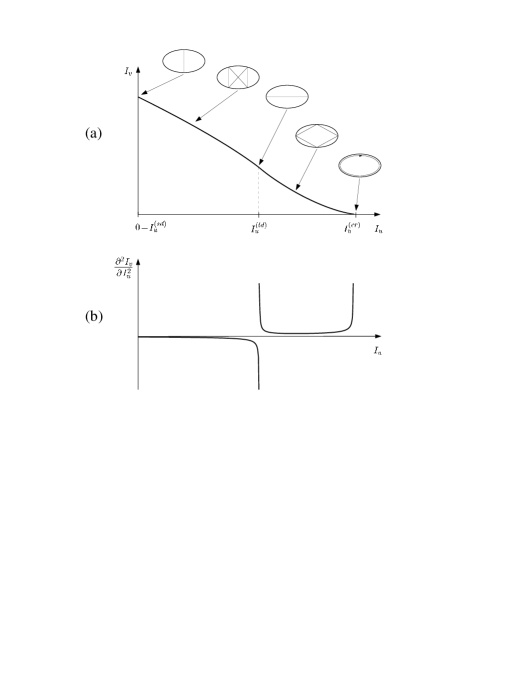
Figure 2: Energy surface $I_{v}(I_{u})$ and curvature $\partial^{2}I_{v}/\partial I_{u}^{2}$ are drawn in the upper and lower panels, respectively, from Ref. [19].

Figure 2(a) shows the energy surface in action space, in the form of the curve $I_{v}=I_{v}(\varepsilon,I_{u})$ at fixed energy $\varepsilon$. Specific primitive orbits (with $M=1$) are illustrated, with the arrows pointing to the corresponding stationary points $I_{u}^{*}$: the short diameter (at $I_{u}^{*}=0$ or $\sigma=0$, with $\Theta_{u}^{*}=0,\pi$), the ‘butterfly’ (or ‘bow-tie’) orbit, the long diameter (at $I_{u}^{*}=I_{u}^{(s)}$, with $\sigma=1$ and $\Theta_{u}^{*}=\pm\pi/2$), the rhomboidal orbits with 4 reflections, and the ‘creeping’ orbit (at $I_{u}^{*}=I_{u}^{\rm(cr)}$) as the limit of a ‘whispering-gallery’ mode with number of reflections $n_{v}=\infty$ and winding number $n_{u}=1$. The limits to the separatrix correspond to infinite values of $n_{v}$ and $n_{u}$ for hyperbolic or elliptic orbits with the ratio $n_{u}/n_{v}$ going to $1/2$ from either side (see also Ref. [14]). We use the same notation for both short and long diameters in terms of the integers $n_{u},n_{v}$ and $M$ like for the elliptic and hyperbolic one-parametric families, specifying them also by the stationary points in the phase space variables $\sigma$ (or $I_{u}$) for all orbits and $\Theta_{u}$ for the isolated ones if necessary.

3.4 Curvature

A key quantity in the semiclassical theory in terms of the action-angle variables is the curvature $K$ of the energy surface

$$K=\frac{\partial^{2}I_{v}}{\partial I_{u}^{2}}=\Big{(}\frac{\partial^{2}I_{v}}{\partial\sigma^{2}}+\frac{\omega_{u}}{\omega_{v}}\frac{\partial^{2}I_{u}}{\partial\sigma^{2}}\Big{)}\Big{/}\Big{(}\frac{\partial I_{u}}{\partial\sigma}\Big{)}^{2}.$$ (19)

The partial derivatives appearing on the right-hand side above are given in Appendix A. Figure 2(b) shows $K$ versus $I_{u}$. In the limit $\sigma\to 0$ one finds the curvature for the twice repeated short diameters considered as primitive orbits [19]. For our definition of the (non-repeated) primitive orbits, one has the curvature $K_{s}$ larger by a factor 2, i.e.,

$$K_{s}=-\frac{1}{\pi pR\eta^{3/2}}$$ (20)

which is finite and negative for all deformations. $K$ stays negative for the entire hyperbolic part $0\leq\sigma<1$ of the curve, whereas it is positive for the elliptic part $1<\sigma<\sigma_{\rm cr}$. At the critical points $\sigma=1$ (separatrix) and at $\sigma_{\rm cr}$ (creeping point), the curvature diverges. It tends to $-\infty$ as one approaches the separatrix from the hyperbolic side, and to $+\infty$ from the elliptic side. For $\sigma\rightarrow\sigma_{\rm cr}$ it also tends to $+\infty$.

4 Phase Space Trace Formula in Action-Angle Variables

4.1 Action-angle variables

We now transform the phase space trace formula (3) from the usual phase space variables $({\mathchoice{\mbox{\boldmath$\displaystyle r$}}{\mbox{\boldmath$\textstyle r$}}{\mbox{\boldmath$\scriptstyle r$}}{\mbox{\boldmath$\scriptstyle r$}}},{\mathchoice{\mbox{\boldmath$\displaystyle p$}}{\mbox{\boldmath$\textstyle p$}}{\mbox{\boldmath$\scriptstyle p$}}{\mbox{\boldmath$\scriptstyle p$}}})$ to the angle-action variables $(\mathchoice{\mbox{\boldmath$\displaystyle\Theta$}}{\mbox{\boldmath$\textstyle\Theta$}}{\mbox{\boldmath$\scriptstyle\Theta$}}{\mbox{\boldmath$\scriptstyle\Theta$}},\mathchoice{\mbox{\boldmath$\displaystyle I$}}{\mbox{\boldmath$\textstyle I$}}{\mbox{\boldmath$\scriptstyle I$}}{\mbox{\boldmath$\scriptstyle I$}})$. The latter are useful for integrable systems because the Hamiltonian $H$ does not depend on the angle variables $\textstyle\Theta$, i.e., $H=H(\mathchoice{\mbox{\boldmath$\displaystyle I$}}{\mbox{\boldmath$\textstyle I$}}{\mbox{\boldmath$\scriptstyle I$}}{\mbox{\boldmath$\scriptstyle I$}})$. For elliptic billiard one has from (3)

$$g_{\rm scl}(\varepsilon)\ = \frac{1}{(2\pi\hbar)^{2}}\mathop{\rm Re}\sum_{\alpha}\int d\Theta_{u}^{\prime\prime}\int d\Theta_{v}^{\prime\prime}\int dI_{u}^{\prime}\int dI_{v}^{\prime}\,\delta(\varepsilon-H(I_{u}^{\prime},I_{v}^{\prime}))$$ (21)

$$\times\exp\left\{\frac{i}{\hbar}\left[S_{\alpha}(\mathchoice{\mbox{\boldmath$\displaystyle I$}}{\mbox{\boldmath$\textstyle I$}}{\mbox{\boldmath$\scriptstyle I$}}{\mbox{\boldmath$\scriptstyle I$}}^{\prime},\mathchoice{\mbox{\boldmath$\displaystyle I$}}{\mbox{\boldmath$\textstyle I$}}{\mbox{\boldmath$\scriptstyle I$}}{\mbox{\boldmath$\scriptstyle I$}}^{\prime\prime},t_{\alpha})+(\mathchoice{\mbox{\boldmath$\displaystyle I$}}{\mbox{\boldmath$\textstyle I$}}{\mbox{\boldmath$\scriptstyle I$}}{\mbox{\boldmath$\scriptstyle I$}}^{\prime\prime}-\mathchoice{\mbox{\boldmath$\displaystyle I$}}{\mbox{\boldmath$\textstyle I$}}{\mbox{\boldmath$\scriptstyle I$}}{\mbox{\boldmath$\scriptstyle I$}}^{\prime})\cdot\mathchoice{\mbox{\boldmath$\displaystyle\Theta$}}{\mbox{\boldmath$\textstyle\Theta$}}{\mbox{\boldmath$\scriptstyle\Theta$}}{\mbox{\boldmath$\scriptstyle\Theta$}}^{\prime\prime}\right]-i\nu_{\alpha}\right\},$$

where $\mathchoice{\mbox{\boldmath$\displaystyle\Theta$}}{\mbox{\boldmath$\textstyle\Theta$}}{\mbox{\boldmath$\scriptstyle\Theta$}}{\mbox{\boldmath$\scriptstyle\Theta$}}=\{\Theta_{u},\Theta_{v}\}$ are the angles and $\mathchoice{\mbox{\boldmath$\displaystyle I$}}{\mbox{\boldmath$\textstyle I$}}{\mbox{\boldmath$\scriptstyle I$}}{\mbox{\boldmath$\scriptstyle I$}}=\{I_{u},I_{v}\}$ the actions for the elliptic billiard defined in the previous section. For simplicity we omitted here and below the Jacobian pre-exponential factor of Eq. (3) because this Jacobian taken at the stationary points is always unity when we apply the improved stationary phase method for the calculation of the integral over phase space variables, as noted above.

4.2 Stationary phase method and classical degeneracy

As noted in the introduction, we emphasize that even for integrable systems the trace integral (21) is more general than the Poisson-sum trace formula which is the starting point of Refs. [4, 5] for the semiclassical derivations. These two trace formulae become identical when we assume that the phase of the exponent also does not depend on the angle variables $\textstyle\Theta$, like the Hamiltonian. Then, the integral over angles in (21) simply gives $(2\pi)^{n}$ where $n$ is the spatial dimension ($n=2$ for the elliptic billiard), see Ref. [5]. In this case the stationary condition for all angle variables are identities in the $2\pi$ interval. This is true for the contribution of the most degenerate classical orbits like elliptic and hyperbolic orbits with ${\cal K}=1$ in the elliptic billiard. For the case of orbits with smaller degeneracy like the isolated diameters (${\cal K}=0$) in the elliptic billiard, the exponent phase is a strongly dependent function of some angles with definite discrete stationary points. We therefore need to integrate over such angles by the standard or improved SPM. Other examples are the equatorial orbits (${\cal K}=1$) and diameters along the symmetry axis (separatrix with ${\cal K}=0)$ in the spheroidal cavity ($n=3$), the degeneracy parameters of which are smaller than the largest possible value ${\cal K}={\cal K}_{\rm max}=2$ for the elliptic and hyperbolic orbits in the meridian plane, or for 3-dimensional orbits. We have a similar situation also for the diameters with ${\cal K}=2$ in the spherical cavity (${\cal K}_{\rm max}=3$), orbits along the symmetry axis for axially-symmetric cavities, and so on. Thus, the stationary conditions with respect to the angle variables for orbits with smaller degeneracies are not identities. Moreover, the stationary points in the cases mentioned above occupy subspaces of the phase space which are isolated in the rational tori that lead to separate contributions to the trace formula, except for the most degenerate orbit families, as we shall see below for the case of the elliptic billiard.

4.3 Stationary phase conditions

We first take the integral over $I_{v}^{\prime}$ in Eq. (21) exactly. Due to the energy conserving $\delta$-function, we are left with the integrals over angles $\Theta_{u}^{\prime\prime}$, $\Theta_{v}^{\prime\prime}$ and action $I_{u}^{\prime}$:

$$g_{\rm scl}(\varepsilon) = \frac{1}{(2\pi\hbar)^{2}}\mathop{\rm Re}\sum_{\alpha}\int d\Theta_{u}^{\prime\prime}\int d\Theta_{v}^{\prime\prime}\int dI_{u}^{\prime}\,\frac{1}{|\omega_{v}^{\prime}|}$$ (22)

$$\times\exp\left[\frac{i}{\hbar}\left(S_{\alpha}(\mathchoice{\mbox{\boldmath$\displaystyle I$}}{\mbox{\boldmath$\textstyle I$}}{\mbox{\boldmath$\scriptstyle I$}}{\mbox{\boldmath$\scriptstyle I$}}^{\prime},\mathchoice{\mbox{\boldmath$\displaystyle I$}}{\mbox{\boldmath$\textstyle I$}}{\mbox{\boldmath$\scriptstyle I$}}{\mbox{\boldmath$\scriptstyle I$}}^{\prime\prime},t_{\alpha})+(\mathchoice{\mbox{\boldmath$\displaystyle I$}}{\mbox{\boldmath$\textstyle I$}}{\mbox{\boldmath$\scriptstyle I$}}{\mbox{\boldmath$\scriptstyle I$}}^{\prime\prime}-\mathchoice{\mbox{\boldmath$\displaystyle I$}}{\mbox{\boldmath$\textstyle I$}}{\mbox{\boldmath$\scriptstyle I$}}{\mbox{\boldmath$\scriptstyle I$}}^{\prime})\cdot\mathchoice{\mbox{\boldmath$\displaystyle\Theta$}}{\mbox{\boldmath$\textstyle\Theta$}}{\mbox{\boldmath$\scriptstyle\Theta$}}{\mbox{\boldmath$\scriptstyle\Theta$}}^{\prime\prime}\right)-i\nu_{\alpha}\right],$$

$$S_{\alpha}(\mathchoice{\mbox{\boldmath$\displaystyle I$}}{\mbox{\boldmath$\textstyle I$}}{\mbox{\boldmath$\scriptstyle I$}}{\mbox{\boldmath$\scriptstyle I$}}^{\prime},\mathchoice{\mbox{\boldmath$\displaystyle I$}}{\mbox{\boldmath$\textstyle I$}}{\mbox{\boldmath$\scriptstyle I$}}{\mbox{\boldmath$\scriptstyle I$}}^{\prime\prime},t_{\alpha})=-\int_{\mathchoice{\mbox{\boldmath$\displaystyle I$}}{\mbox{\boldmath$\textstyle I$}}{\mbox{\boldmath$\scriptstyle I$}}{\mbox{\boldmath$\scriptstyle I$}}^{\prime}}^{\mathchoice{\mbox{\boldmath$\displaystyle I$}}{\mbox{\boldmath$\textstyle I$}}{\mbox{\boldmath$\scriptstyle I$}}{\mbox{\boldmath$\scriptstyle I$}}^{\prime\prime}}d\mathchoice{\mbox{\boldmath$\displaystyle I$}}{\mbox{\boldmath$\textstyle I$}}{\mbox{\boldmath$\scriptstyle I$}}{\mbox{\boldmath$\scriptstyle I$}}\cdot\mathchoice{\mbox{\boldmath$\displaystyle\Theta$}}{\mbox{\boldmath$\textstyle\Theta$}}{\mbox{\boldmath$\scriptstyle\Theta$}}{\mbox{\boldmath$\scriptstyle\Theta$}}(\mathchoice{\mbox{\boldmath$\displaystyle I$}}{\mbox{\boldmath$\textstyle I$}}{\mbox{\boldmath$\scriptstyle I$}}{\mbox{\boldmath$\scriptstyle I$}}).$$ (23)

We first write down the stationary phase equation for $I_{u}$:

$$\left(\frac{\partial S_{\alpha}(\mathchoice{\mbox{\boldmath$\displaystyle I$}}{\mbox{\boldmath$\textstyle I$}}{\mbox{\boldmath$\scriptstyle I$}}{\mbox{\boldmath$\scriptstyle I$}}^{\prime},\mathchoice{\mbox{\boldmath$\displaystyle I$}}{\mbox{\boldmath$\textstyle I$}}{\mbox{\boldmath$\scriptstyle I$}}{\mbox{\boldmath$\scriptstyle I$}}^{\prime\prime},t_{\alpha})}{\partial I_{u}^{\prime}}\right)^{*}-\Theta_{u}^{\prime\prime}\equiv\Theta_{u}^{\prime}-\Theta_{u}^{\prime\prime}=2\pi M_{u},$$ (24)

where $M_{u}$ is an integer. The star means that we take the quantities at the stationary point $I_{u}^{\prime}=I_{u}^{*}$. We now use the Legendre transformation (6), which reads

$$S_{\alpha}(\mathchoice{\mbox{\boldmath$\displaystyle I$}}{\mbox{\boldmath$\textstyle I$}}{\mbox{\boldmath$\scriptstyle I$}}{\mbox{\boldmath$\scriptstyle I$}}^{\prime},\mathchoice{\mbox{\boldmath$\displaystyle I$}}{\mbox{\boldmath$\textstyle I$}}{\mbox{\boldmath$\scriptstyle I$}}{\mbox{\boldmath$\scriptstyle I$}}^{\prime\prime},t_{\alpha})+(\mathchoice{\mbox{\boldmath$\displaystyle I$}}{\mbox{\boldmath$\textstyle I$}}{\mbox{\boldmath$\scriptstyle I$}}{\mbox{\boldmath$\scriptstyle I$}}^{\prime\prime}-\mathchoice{\mbox{\boldmath$\displaystyle I$}}{\mbox{\boldmath$\textstyle I$}}{\mbox{\boldmath$\scriptstyle I$}}{\mbox{\boldmath$\scriptstyle I$}}^{\prime})\cdot\mathchoice{\mbox{\boldmath$\displaystyle\Theta$}}{\mbox{\boldmath$\textstyle\Theta$}}{\mbox{\boldmath$\scriptstyle\Theta$}}{\mbox{\boldmath$\scriptstyle\Theta$}}^{\prime\prime}=S_{\alpha}(\mathchoice{\mbox{\boldmath$\displaystyle\Theta$}}{\mbox{\boldmath$\textstyle\Theta$}}{\mbox{\boldmath$\scriptstyle\Theta$}}{\mbox{\boldmath$\scriptstyle\Theta$}}^{\prime\prime},\mathchoice{\mbox{\boldmath$\displaystyle\Theta$}}{\mbox{\boldmath$\textstyle\Theta$}}{\mbox{\boldmath$\scriptstyle\Theta$}}{\mbox{\boldmath$\scriptstyle\Theta$}}^{\prime},\varepsilon)-\mathchoice{\mbox{\boldmath$\displaystyle I$}}{\mbox{\boldmath$\textstyle I$}}{\mbox{\boldmath$\scriptstyle I$}}{\mbox{\boldmath$\scriptstyle I$}}^{\prime}\cdot(\mathchoice{\mbox{\boldmath$\displaystyle\Theta$}}{\mbox{\boldmath$\textstyle\Theta$}}{\mbox{\boldmath$\scriptstyle\Theta$}}{\mbox{\boldmath$\scriptstyle\Theta$}}^{\prime\prime}-\mathchoice{\mbox{\boldmath$\displaystyle\Theta$}}{\mbox{\boldmath$\textstyle\Theta$}}{\mbox{\boldmath$\scriptstyle\Theta$}}{\mbox{\boldmath$\scriptstyle\Theta$}}^{\prime}),$$ (25)

$$S_{\alpha}(\mathchoice{\mbox{\boldmath$\displaystyle\Theta$}}{\mbox{\boldmath$\textstyle\Theta$}}{\mbox{\boldmath$\scriptstyle\Theta$}}{\mbox{\boldmath$\scriptstyle\Theta$}}^{\prime},\mathchoice{\mbox{\boldmath$\displaystyle\Theta$}}{\mbox{\boldmath$\textstyle\Theta$}}{\mbox{\boldmath$\scriptstyle\Theta$}}{\mbox{\boldmath$\scriptstyle\Theta$}}^{\prime\prime},\varepsilon)=\int_{\mathchoice{\mbox{\boldmath$\displaystyle\Theta$}}{\mbox{\boldmath$\textstyle\Theta$}}{\mbox{\boldmath$\scriptstyle\Theta$}}{\mbox{\boldmath$\scriptstyle\Theta$}}^{\prime}}^{\mathchoice{\mbox{\boldmath$\displaystyle\Theta$}}{\mbox{\boldmath$\textstyle\Theta$}}{\mbox{\boldmath$\scriptstyle\Theta$}}{\mbox{\boldmath$\scriptstyle\Theta$}}^{\prime\prime}}d\mathchoice{\mbox{\boldmath$\displaystyle\Theta$}}{\mbox{\boldmath$\textstyle\Theta$}}{\mbox{\boldmath$\scriptstyle\Theta$}}{\mbox{\boldmath$\scriptstyle\Theta$}}\cdot\mathchoice{\mbox{\boldmath$\displaystyle I$}}{\mbox{\boldmath$\textstyle I$}}{\mbox{\boldmath$\scriptstyle I$}}{\mbox{\boldmath$\scriptstyle I$}}(\mathchoice{\mbox{\boldmath$\displaystyle\Theta$}}{\mbox{\boldmath$\textstyle\Theta$}}{\mbox{\boldmath$\scriptstyle\Theta$}}{\mbox{\boldmath$\scriptstyle\Theta$}}).$$

With the use of this transformation, the stationary phase conditions for angles $\Theta_{u}$ and $\Theta_{v}$ are written as

$$\left(\frac{\partial S_{\alpha}(\mathchoice{\mbox{\boldmath$\displaystyle\Theta$}}{\mbox{\boldmath$\textstyle\Theta$}}{\mbox{\boldmath$\scriptstyle\Theta$}}{\mbox{\boldmath$\scriptstyle\Theta$}}^{\prime},\mathchoice{\mbox{\boldmath$\displaystyle\Theta$}}{\mbox{\boldmath$\textstyle\Theta$}}{\mbox{\boldmath$\scriptstyle\Theta$}}{\mbox{\boldmath$\scriptstyle\Theta$}}^{\prime\prime},\varepsilon)}{\partial\mathchoice{\mbox{\boldmath$\displaystyle\Theta$}}{\mbox{\boldmath$\textstyle\Theta$}}{\mbox{\boldmath$\scriptstyle\Theta$}}{\mbox{\boldmath$\scriptstyle\Theta$}}^{\prime\prime}}+\frac{\partial S_{\alpha}(\mathchoice{\mbox{\boldmath$\displaystyle\Theta$}}{\mbox{\boldmath$\textstyle\Theta$}}{\mbox{\boldmath$\scriptstyle\Theta$}}{\mbox{\boldmath$\scriptstyle\Theta$}}^{\prime},\mathchoice{\mbox{\boldmath$\displaystyle\Theta$}}{\mbox{\boldmath$\textstyle\Theta$}}{\mbox{\boldmath$\scriptstyle\Theta$}}{\mbox{\boldmath$\scriptstyle\Theta$}}^{\prime\prime},\varepsilon)}{\partial\mathchoice{\mbox{\boldmath$\displaystyle\Theta$}}{\mbox{\boldmath$\textstyle\Theta$}}{\mbox{\boldmath$\scriptstyle\Theta$}}{\mbox{\boldmath$\scriptstyle\Theta$}}^{\prime}}\right)^{*}\equiv\mathchoice{\mbox{\boldmath$\displaystyle I$}}{\mbox{\boldmath$\textstyle I$}}{\mbox{\boldmath$\scriptstyle I$}}{\mbox{\boldmath$\scriptstyle I$}}^{\prime\prime}-\mathchoice{\mbox{\boldmath$\displaystyle I$}}{\mbox{\boldmath$\textstyle I$}}{\mbox{\boldmath$\scriptstyle I$}}{\mbox{\boldmath$\scriptstyle I$}}^{\prime}=0.$$ (26)

For the following derivations we have to decide which stationary phase conditions from Eqs. (24) and (26) are identities for the finite volume of the phase-space tori and which are equations for the isolated stationary points. For doing this, we have to calculate separately the contributions from the most degenerate (elliptic and hyperbolic) families $({\cal K}=1)$ to the improved trace formula and those from diameters in the elliptic billiard. These two contributions are different with respect to the above mentioned decision concerning the integration over the angles $\textstyle\Theta$. After the integration over one of the angle variables, say $\Theta_{v}$, corresponding to the identity in the stationary phase conditions (26) due to an invariance of the action along the periodic orbit in Eq. (22), one gets Eq. (7) of Ref. [30] derived earlier by Bruno [38]. So, we get the result of Refs. [30, 38] within periodic orbit theory. Our phase-space trace formula (3) is more general because it can be applied for more exact calculations of the level density, without use of the stationary phase conditions like Eqs.(26), in terms of closed (periodic and non-periodic) orbits.

Note that we have separate contributions coming from each kind of families and isolated orbits even near the bifurcation points (18) where we have the end point. Taking the deformation at a small distance from $\eta_{\rm bif}$, we are left with two separate close stationary points and then use the Maslov-Fedoryuk theory [39, 40, 41, 42] like for caustic and turning points. Finally, after the integration by the improved stationary phase method, we look at the limit $\eta\rightarrow\eta_{\rm bif}$ to the bifurcation point. In particular, this idea of Maslov and Fedoryuk was applied in Appendix B for the calculation of the contribution of the long diameter at the separatrix.

5 Trace Formulas for the Elliptic Billiard

5.1 Elliptic and hyperbolic orbit families $({\cal K}=n-1=1)$

Each family of elliptic or hyperbolic orbits with a common action occupies a two-dimensional finite area in the elliptic billiard. In this case, the stationary conditions (26) for the integration over the angle variables $\Theta_{u}$ and $\Theta_{v}$ become identities, since the integrand does not depend on the angle variables, and we have the conservation of the action variable $I_{u}^{\prime}=I_{u}^{\prime\prime}=I_{u}$ fulfilled identically along each classical trajectory $\alpha$. Taking the integrals over $\textstyle\Theta$ gives a factor $(2\pi)^{2}$, and we are left with the Poisson-sum trace formula like in Refs. [4, 5]:

$$g_{\rm scl}(\varepsilon) = \frac{1}{\hbar^{2}}\mathop{\rm Re}\sum_{\mathchoice{\mbox{\boldmath$\displaystyle M$}}{\mbox{\boldmath$\textstyle M$}}{\mbox{\boldmath$\scriptstyle M$}}{\mbox{\boldmath$\scriptstyle M$}}}\int d\mathchoice{\mbox{\boldmath$\displaystyle I$}}{\mbox{\boldmath$\textstyle I$}}{\mbox{\boldmath$\scriptstyle I$}}{\mbox{\boldmath$\scriptstyle I$}}\>\delta(\varepsilon-H(\mathchoice{\mbox{\boldmath$\displaystyle I$}}{\mbox{\boldmath$\textstyle I$}}{\mbox{\boldmath$\scriptstyle I$}}{\mbox{\boldmath$\scriptstyle I$}}))\exp\left[\frac{2\pi i}{\hbar}\mathchoice{\mbox{\boldmath$\displaystyle M$}}{\mbox{\boldmath$\textstyle M$}}{\mbox{\boldmath$\scriptstyle M$}}{\mbox{\boldmath$\scriptstyle M$}}\cdot\mathchoice{\mbox{\boldmath$\displaystyle I$}}{\mbox{\boldmath$\textstyle I$}}{\mbox{\boldmath$\scriptstyle I$}}{\mbox{\boldmath$\scriptstyle I$}}-i\nu_{\mathchoice{\mbox{\boldmath$\displaystyle M$}}{\mbox{\boldmath$\textstyle M$}}{\mbox{\boldmath$\scriptstyle M$}}{\mbox{\boldmath$\scriptstyle M$}}}\right]$$ (27)

$$= \frac{1}{\hbar^{2}}\mathop{\rm Re}\sum_{\mathchoice{\mbox{\boldmath$\displaystyle M$}}{\mbox{\boldmath$\textstyle M$}}{\mbox{\boldmath$\scriptstyle M$}}{\mbox{\boldmath$\scriptstyle M$}}}\int dI_{u}\>\frac{1}{|\omega_{v}|}\exp\left[\frac{2\pi i}{\hbar}\mathchoice{\mbox{\boldmath$\displaystyle M$}}{\mbox{\boldmath$\textstyle M$}}{\mbox{\boldmath$\scriptstyle M$}}{\mbox{\boldmath$\scriptstyle M$}}\cdot\mathchoice{\mbox{\boldmath$\displaystyle I$}}{\mbox{\boldmath$\textstyle I$}}{\mbox{\boldmath$\scriptstyle I$}}{\mbox{\boldmath$\scriptstyle I$}}-i\nu_{\mathchoice{\mbox{\boldmath$\displaystyle M$}}{\mbox{\boldmath$\textstyle M$}}{\mbox{\boldmath$\scriptstyle M$}}{\mbox{\boldmath$\scriptstyle M$}}}\right].$$

Here $\mathchoice{\mbox{\boldmath$\displaystyle M$}}{\mbox{\boldmath$\textstyle M$}}{\mbox{\boldmath$\scriptstyle M$}}{\mbox{\boldmath$\scriptstyle M$}}=(M_{u},M_{v})$ are integers which correspond to those in Eq. (14). Next we transform the integration variable in the last expression of Eq. (27) from $I_{u}$ to $\sigma$ defined by (9). Thus, the level density component $\delta g_{{\rm scl},1}$ related to the one-parameter families can be written as a sum of contributions from the hyperbolic ($\delta g_{{\rm scl},1}^{(h)}(\varepsilon)$) and the elliptic ($\delta g_{{\rm scl},1}^{(e)}(\varepsilon)$) parts of the tori. Their sum is

$$\delta g_{{\rm scl},1}(\varepsilon)=\frac{1}{\pi\varepsilon_{0}pR^{2}}\mathop{\rm Re}\!\sum_{\mathchoice{\mbox{\boldmath$\displaystyle M$}}{\mbox{\boldmath$\textstyle M$}}{\mbox{\boldmath$\scriptstyle M$}}{\mbox{\boldmath$\scriptstyle M$}}}\frac{1}{n_{v}}\!\int_{0}^{\sigma_{\rm cr}}\!\!d\sigma L_{\mathchoice{\mbox{\boldmath$\displaystyle M$}}{\mbox{\boldmath$\textstyle M$}}{\mbox{\boldmath$\scriptstyle M$}}{\mbox{\boldmath$\scriptstyle M$}}}\frac{\partial I_{u}}{\partial\sigma}\exp\!\!\left[\frac{2\pi i}{\hbar}\mathchoice{\mbox{\boldmath$\displaystyle M$}}{\mbox{\boldmath$\textstyle M$}}{\mbox{\boldmath$\scriptstyle M$}}{\mbox{\boldmath$\scriptstyle M$}}\!\cdot\!\mathchoice{\mbox{\boldmath$\displaystyle I$}}{\mbox{\boldmath$\textstyle I$}}{\mbox{\boldmath$\scriptstyle I$}}{\mbox{\boldmath$\scriptstyle I$}}(\sigma)-i\nu_{\mathchoice{\mbox{\boldmath$\displaystyle M$}}{\mbox{\boldmath$\textstyle M$}}{\mbox{\boldmath$\scriptstyle M$}}{\mbox{\boldmath$\scriptstyle M$}}}\right]\!,$$ (28)

where $\varepsilon_{0}=\hbar^{2}/(2mR^{2})$, $\mathchoice{\mbox{\boldmath$\displaystyle I$}}{\mbox{\boldmath$\textstyle I$}}{\mbox{\boldmath$\scriptstyle I$}}{\mbox{\boldmath$\scriptstyle I$}}(\sigma)$ are the actions defined by Eqs. (11), $L_{\mathchoice{\mbox{\boldmath$\displaystyle M$}}{\mbox{\boldmath$\textstyle M$}}{\mbox{\boldmath$\scriptstyle M$}}{\mbox{\boldmath$\scriptstyle M$}}}$ are the ‘lengths’ of the primitive orbits with $M=1$ given by

$$L_{\mathchoice{\mbox{\boldmath$\displaystyle M$}}{\mbox{\boldmath$\textstyle M$}}{\mbox{\boldmath$\scriptstyle M$}}{\mbox{\boldmath$\scriptstyle M$}}} = \frac{2\pi n_{v}p}{m\omega_{v}}$$ (29)

$$= 2n_{v}b\,\sin{\theta}\!\left[\mathop{\rm E}(\theta,\kappa)-\frac{\mathop{\rm F}(\theta,\kappa)}{\mathop{\rm F}(\frac{\pi}{2},\kappa)}\,\mathop{\rm E}({\textstyle\frac{\pi}{2}},\kappa)+\cot\theta\sqrt{1-\kappa^{2}\sin^{2}\theta}\right],$$

and $\theta(\sigma)$ and $\kappa(\sigma)$ are defined by Eq. (15). The ‘lengths’ become the true lengths of the corresponding periodic orbits when they are taken at $\sigma$ equal to the real positive roots of Eq. (12) inside the integration range. For other values of $\sigma$, the ‘lengths’ are nothing else than the functions (29) introduced in place of $\omega_{v}$ for convenience. The integration range from the bifurcation point $\sigma=0$ to the separatrix $\sigma_{s}=1$ covers the contributions of all hyperbolic orbits. The remaining part of Eq. (28) from $\sigma=1$ to the creeping value $\sigma_{\rm cr}$ gives the contributions from the elliptic tori.

As we shall see below, the choice of $\sigma$ as the integration variable significantly improves the precision of the SPM. We hence apply the stationary condition (24) for the phase in the integrands of Eq. (28) with respect to $\sigma$ rather than to $I_{u}$. With Eqs. (15), this condition becomes identical to Eq. (12) and determines the stationary phase point $\sigma^{\prime}=\sigma^{\prime\prime}=\sigma^{*}$ related to $I_{u}^{\prime}=I_{u}^{\prime\prime}=I_{u}^{*}$. We used here the conservation of $\sigma$ (or the additional integral of motion $l_{+}l_{-}$) along the periodic orbit. We now expand the phase up to second order,

$$S_{\alpha}(\mathchoice{\mbox{\boldmath$\displaystyle I$}}{\mbox{\boldmath$\textstyle I$}}{\mbox{\boldmath$\scriptstyle I$}}{\mbox{\boldmath$\scriptstyle I$}}^{\prime},\mathchoice{\mbox{\boldmath$\displaystyle I$}}{\mbox{\boldmath$\textstyle I$}}{\mbox{\boldmath$\scriptstyle I$}}{\mbox{\boldmath$\scriptstyle I$}}^{\prime\prime},t_{\alpha})+(\mathchoice{\mbox{\boldmath$\displaystyle I$}}{\mbox{\boldmath$\textstyle I$}}{\mbox{\boldmath$\scriptstyle I$}}{\mbox{\boldmath$\scriptstyle I$}}^{\prime\prime}-\mathchoice{\mbox{\boldmath$\displaystyle I$}}{\mbox{\boldmath$\textstyle I$}}{\mbox{\boldmath$\scriptstyle I$}}{\mbox{\boldmath$\scriptstyle I$}}^{\prime})\cdot\mathchoice{\mbox{\boldmath$\displaystyle\Theta$}}{\mbox{\boldmath$\textstyle\Theta$}}{\mbox{\boldmath$\scriptstyle\Theta$}}{\mbox{\boldmath$\scriptstyle\Theta$}}^{\prime\prime}=2\pi\mathchoice{\mbox{\boldmath$\displaystyle M$}}{\mbox{\boldmath$\textstyle M$}}{\mbox{\boldmath$\scriptstyle M$}}{\mbox{\boldmath$\scriptstyle M$}}\cdot\mathchoice{\mbox{\boldmath$\displaystyle I$}}{\mbox{\boldmath$\textstyle I$}}{\mbox{\boldmath$\scriptstyle I$}}{\mbox{\boldmath$\scriptstyle I$}}=S_{\beta}(\varepsilon)+\frac{1}{2}J_{\beta}^{\parallel}(\sigma-\sigma^{*})^{2},$$ (30)

where $S_{\beta}$ is the action along the periodic orbit $\beta$ determined by Eq. (12),

$$S_{\beta}(\varepsilon)=2\pi M(n_{u}I_{u}(\sigma^{*})+n_{v}I_{v}(\sigma^{*})),$$ (31)

and $J_{\beta}^{\parallel}$ is the Jacobian stability factor with respect to $\sigma$ along the energy surface:

$$J_{\beta}^{\parallel}=\left(\frac{\partial^{2}S}{\partial\sigma^{2}}\right)_{\sigma=\sigma^{*},\beta}=2\pi M\left(n_{u}\frac{\partial^{2}I_{u}}{\partial\sigma^{2}}+n_{v}\frac{\partial^{2}I_{v}}{\partial\sigma^{2}}\right)_{\sigma=\sigma^{*},\beta}.$$ (32)

It is related to the curvature $K_{\beta}$ (19) of the energy surface by

$$J_{\beta}^{\parallel}=2\pi Mn_{v}K_{\beta}\left(\frac{\partial I_{u}}{\partial\sigma}\right)^{2}_{\sigma=\sigma^{*},\beta}=2\pi Mn_{v}\epsilon\left|K_{\beta}\right|\left(\frac{\partial I_{u}}{\partial\sigma}\right)^{2}_{\sigma=\sigma^{*},\beta},$$ (33)

where $\epsilon=+1$ for elliptic orbits and $\epsilon=-1$ for hyperbolic orbits. We substitute now the expansion (30) and take the pre-exponential factor off the integral in Eq. (28). For the sake of simplicity, we only consider the lowest order in the expansion of the phase and the pre-exponential factor in Eq. (28) in the variable $\sigma$, although higher-order expansions can in principle be used to improve the precision of the SPM. Thus, we are left with the integral from $\sigma=0$ to $1$ for the hyperbolic orbits, and from $\sigma=1$ to $\sigma_{\rm cr}$ for the elliptic orbits.

When the stationary point $\sigma^{*}$ is far from the limits of these intervals, one can extend the integration range from $-\infty$ to $\infty$ and get the result of the standard POT [4]. Near the bifurcation points (18) of the short diameter orbit (where the hyperbolic orbit families appear), however, the stationary point $\sigma^{*}$ is close to zero. In this case we cannot extend the lower limit to $-\infty$ but have to take the integral exactly from $\sigma=0$. On the other hand, when the stationary point $\sigma^{*}$ approaches the integration limits $\sigma_{s}$ (16) or $\sigma_{\rm cr}$ (17), hyperbolic or elliptic orbits with an increasing number of corners $n_{v}$ appear. In these cases, too, we cannot extend the integration limits to $\pm\infty$. Taking the integral over $\sigma$ within the finite limits, we obtain a trace formula in terms of complex Fresnel functions or generalized error functions. The contributions of the one-parameter orbit families $\delta g_{{\rm scl},1}(\varepsilon)$ are then given in the form

$$\delta g_{{\rm scl},1}(\varepsilon)=\mathop{\rm Re}\sum_{\beta}{\cal A}_{\beta}^{(1)}(\varepsilon)\exp\left[ikL_{\beta}-i\nu_{\beta}^{\rm(tot)}\right].$$ (34)

Here, the sum is taken over both elliptic and hyperbolic orbit families, $k=\sqrt{2m\varepsilon}/\hbar$. The amplitude ${\cal A}_{\beta}^{(1)}$ of the orbit family $\beta$ is given by

$${\cal A}_{\beta}^{(1)}=\frac{L_{\beta}}{2\varepsilon_{0}\pi kR^{2}\sqrt{-\epsilon iM^{3}n_{v}^{3}\left|\hbar K_{\beta}\right|}}\mathop{\rm erf}\left({\cal Z}_{\beta,1}^{\parallel},{\cal Z}_{\beta,2}^{\parallel}\right);$$ (35)

$L_{\beta}$ is the ‘length’ of the orbit family (29) corresponding to the stationary point $\sigma^{*}$ ($M=1$). We have introduced here the generalized error function $\mathop{\rm erf}(z_{1},z_{2})$:

$$\mathop{\rm erf}(z_{1},z_{2})=\frac{2}{\sqrt{\pi}}\int_{z_{1}}^{z_{2}}dze^{-z^{2}}=\mathop{\rm erf}(z_{2})-\mathop{\rm erf}(z_{1}),$$ (36)

$\mathop{\rm erf}(z)$ being the standard error function [47] with (complex) argument $z$. The complex quantities ${\cal Z}_{\beta,1}^{\parallel}$ and ${\cal Z}_{\beta,2}^{\parallel}$ in (35) are given in terms of the Jacobian $J_{\beta}^{\parallel}$ (32) and the stationary points $\sigma^{*}$:

$${\cal Z}_{\beta,1}^{\parallel}=\sqrt{\frac{\epsilon i|J_{\beta}^{\parallel}|}{2\hbar}}\left(\sigma_{\rm min}^{(\epsilon)}-\sigma^{*}\right),\qquad{\cal Z}_{\beta,2}^{\parallel}=\sqrt{\frac{\epsilon i|J_{\beta}^{\parallel}|}{2\hbar}}\left(\sigma_{\rm max}^{(\epsilon)}-\sigma^{*}\right),$$ (37)

where $\sigma_{\rm min}^{(\epsilon)}$ and $\sigma_{\rm max}^{(\epsilon)}$ are related to the integration limits by

$$\sigma_{\rm min}^{(\epsilon)}=\left\{\begin{array}[]{c@{,\quad}l}1&\epsilon=1\\ 0&\epsilon=-1\end{array}\right\},\qquad\sigma_{\rm max}^{(\epsilon)}=\left\{\begin{array}[]{c@{,\quad}l}\sigma_{\rm cr}&\epsilon=1\\ 1&\epsilon=-1\end{array}\right\}.$$ (38)

The phases $\nu_{\beta}^{\rm(tot)}$ in (34) are related to the Maslov indices. They have a constant part $\nu_{\beta}$ which is independent of deformation $\eta$ and energy $\varepsilon$. At deformations which are far enough from bifurcation points, such that the stationary points are far enough from the integration limits, we can determine this asymptotic part $\nu_{\beta}$ by transforming the error functions to Fresnel functions [47] with real limits and extending the integration limits to $\pm\infty$. We hereby arrive at the amplitude ${\cal A}_{\beta}^{(1)}$ of the standard POT [4, 11, 44]

$${\cal A}_{\beta}^{(1)}=\frac{L_{\beta}}{\varepsilon_{0}\pi kR^{2}\sqrt{-\epsilon iM^{3}n_{v}^{3}\left|\hbar K_{\beta}\right|}},$$ (39)

and $\nu_{\beta}$ is determined by the number of turning and caustic points as in the theory of Maslov and Fedoryuk [39, 40, 41, 42]. In terms of the numbers $n_{v}$ and $n_{u}$ and the repetition number $M$, it is given by

$$\nu_{\beta} = \displaystyle\frac{3}{\pi}2n_{v}M\hskip 62.0pt\mbox{for $\epsilon=+1$},$$

$$\nu_{\beta} = \displaystyle\frac{\pi}{2}(2n_{u}+2n_{v})M\qquad\mbox{for $\epsilon=-1$}.$$ (40)

¿From Eqs. (34), (35), and (40) we determine an extra contribution to the total phase $\nu_{\beta}^{\rm(tot)}$

$$\nu_{\beta}^{\rm(tot)}=\nu_{\beta}^{\rm(tot)}(\eta,kR)=\nu_{\beta}-\frac{\pi}{4}\epsilon-\mathop{\rm arg}\left\{\mathop{\rm erf}\left({\cal Z}_{\beta,1}^{\parallel},{\cal Z}_{\beta,2}^{\parallel}\right)\right\}$$ (41)

that analytically connects the asymptotic values $\nu_{\beta}$ and depends on the energy through $kR$. The final result (41) for the total phase depends also on the deformation parameter $\eta$.

Note that $\sigma^{*}$ is negative for $\eta\!<\!\eta_{\rm bif}$. In the derivation of Eqs. (34) and (35), we have changed the integration variable from $\sigma$ to $z\!=\!\sqrt{-i\epsilon|J_{\beta}^{\parallel}|/(2\hbar)}(\sigma-\sigma^{*})$ in order to transfer the $kR$ and $\eta$ dependence of the integrand to the limits of the complex generalized error functions (36). Note also that our energy and deformation dependent phase $\nu_{\beta}^{\rm(tot)}$ is essentially different from Ref. [26] and much simpler in its analytical structure. Different from Refs. [26, 29], we did not use any assumption concerning a smoothness of the phase. Our solution is regular at the separatrix and creeping points, at all bifurcations points and in the circular disk limit. We easily get the correct circular disk limit [46] and the Berry-Tabor result [4] for larger deformations far from the bifurcations.

Equations (34), (35) and (41) represent one of our central results concerning the contributions of the degenerate orbit families (${\cal K}=1$), that simultaneously solves the symmetry-breaking problem for both hyperbolic and elliptic orbits: near $\eta=1$ and other bifurcation points for all hyperbolic orbits, and near the separatrix $\sigma_{s}$ and the ‘creeping’ point $\sigma_{\rm cr}$ for all elliptic orbits. The additional contributions of the isolated orbits (${\cal K}=0$) will be derived in the two following subsections.

Formally, our result (34) coincides with the first main term of the Berry-Tabor trace formula, see Eq. (24) of Ref. [4], using the simplest way of the expansions near the stationary point instead of a more general and more complicated mapping procedure. The next two terms of their formula, being of higher order in $\sqrt{\hbar}$, can be obtained by accounting for the linear term in the expansion of the pre-exponential factor over $\sigma-\sigma^{*}$. They were neglected in our approach because we are interested here only in the main term of the SPM expansion, in order to get the simplest possible solution of the bifurcation problem. With the higher-order corrections, we should take into account that the ratio of the contribution of the linear term to the zero-order term of the amplitude is of the same order as the relative contribution of the next order (cubic) term in the expansion of the phase. For a consistent treatment of the level density in the semiclassical asymptotic approximation $kR\gg 1$, one would have to collect both corrections.

5.2 Short diametric orbits $({\cal K}=0)$

For the contribution of the isolated (${\cal K}=0$) diameters, only one of the two stationary phase conditions (26) corresponding to the $\Theta_{v}$ variable is an identity. The other one for $\Theta_{u}$ is a nontrivial equation for the discrete number of the stationary points which differ by integer multiple of $\pi$. Indeed, due to the integrability of motion in the elliptic billiard one has

$$\Theta_{u}=\omega_{u}t+\Theta_{u}^{(0)},\qquad\Theta_{v}=\omega_{v}t+\Theta_{v}^{(0)},$$ (42)

where $\mathchoice{\mbox{\boldmath$\displaystyle\Theta$}}{\mbox{\boldmath$\textstyle\Theta$}}{\mbox{\boldmath$\scriptstyle\Theta$}}{\mbox{\boldmath$\scriptstyle\Theta$}}^{(0)}$ is the initial angle $\textstyle\Theta$ at $t=0$. Since the frequency $\omega_{u}$ in Eqs. (42) is zero for short diameters, for instance, there is no room for an identity in the stationary phase condition for the variable $\Theta_{u}$ in Eq. (22). Hence, the Poisson-sum trace formula cannot be applied to get the contribution from the short diameters unlike in the derivations in Ref. [24]. The stationary points for the integration in Eq. (22) over angle $\Theta_{u}$ for the short diameters are constants $\Theta_{u}^{*}=\pi M$ for $M=0,\pm 1,\ldots$. Due to the periodicity of the angle variable with the period $2\pi$ we really need to deal with the two stationary points $\Theta_{u}^{*}=0$ and $\pi$ in the integration interval from $-\pi$ to $\pi$ over the angle $\Theta_{u}$ in Eq. (22). We can then reduce the initial integration interval for angle variable $\Theta_{u}$ to the region from $-\pi/2$ to $\pi/2$ taking into account the integration over other angles (related to the motion along the same periodic orbit in the opposite direction) by the factor 2 (due to the time reversal invariance of the Hamiltonian). Within this reduced integration interval, only one stationary point $\Theta_{u}^{*}=0$ must be taken into account in the calculation by the improved stationary phase method.

For the other variable $\Theta_{v}$ for the short diameters we have identity in the corresponding equation from Eq. (26). The integrand in (22) is independent of the variable $\Theta_{v}$ and the integral gives simply $2\pi$. Thus, the integrand for the contribution of the short diameters essentially depends only on $\Theta_{u}$ and possesses the relevant stationary points. When we take this integral by the SSPM we get immediately Gutzwiller’s result for the short diameters with his stability factor in the denominator. This stability factor is zero at the bifurcation points. We shall below get the short diameter term improved at the bifurcation points. For this purpose we shall first follow the same method in the integration over $\Theta_{u}$ and $I_{u}$ as we did in the integration over $I_{u}$ for elliptic and hyperbolic orbits with highest degeneracies. The integration interval over $I_{u}$ for the contribution of the short diameters is also finite from 0 to the maximal “creeping” value $I_{u}^{\rm(cr)}$ (17) which corresponds to the region of the $\sigma$ variable $0\leq\sigma\leq\sigma_{\rm cr}$.

Thus, for the short diameters, we use the stationary condition for the angle variable $\Theta_{u}$ and expand the phase of exponent in Eq. (22) about the short diameter,

$$S_{\alpha}=S_{sM}(\varepsilon)+\frac{1}{2}J_{sM}^{\perp}\Theta_{u}^{2},$$ (43)

with $S_{sM}(\varepsilon)$ being the action along the short diameter, $S_{sM}(\varepsilon)=4\,p(\varepsilon)\,aM$ and $\Theta_{u}^{*}=0$. $J_{sM}^{\perp}$ is the Jacobian corresponding to the second variation of the action $S_{\alpha}$ with respect to the angle variable $\Theta_{u}$,

$$J_{sM}^{\perp} = \left(\frac{\partial^{2}S_{\alpha}}{\partial\Theta_{u}^{\prime 2}}+2\frac{\partial^{2}S_{\alpha}}{\partial\Theta_{u}^{\prime}\partial\Theta_{u}^{\prime\prime}}+\frac{\partial^{2}S_{\alpha}}{\partial\Theta_{u}^{\prime\prime 2}}\right)_{sM}=\left(-\frac{\partial I_{u}^{\prime}}{\partial\Theta_{u}^{\prime}}-2\frac{\partial I_{u}^{\prime}}{\partial\Theta_{u}^{\prime\prime}}+\frac{\partial I_{u}^{\prime\prime}}{\partial\Theta_{u}^{\prime\prime}}\right)_{sM},$$

according to Eq. (25). The Jacobian $J_{sM}^{\perp}$ is expressed in terms of the diametric curvature $K_{s}$ (20) and Gutzwiller’s stability factor $F_{sM}$,

$$F_{sM}=-\left(\frac{-\frac{\partial I_{u}^{\prime}}{\partial\Theta_{u}^{\prime}}-2\frac{\partial I_{u}^{\prime}}{\partial\Theta_{u}^{\prime\prime}}+\frac{\partial I_{u}^{\prime\prime}}{\partial\Theta_{u}^{\prime\prime}}}{\frac{\partial I_{u}^{\prime}}{\partial\Theta_{u}^{\prime\prime}}}\right)_{sM}=4\sin^{2}\left[M\arccos(2\eta^{-2}-1)\right],$$ (45)

which is independent of the choice of the phase space variables

$$J_{sM}^{\perp}=F_{sM}J_{sM}^{(\Theta)}=-\frac{F_{sM}}{4\pi MK_{s}},$$ (46)

where

$$J_{sM}^{(\Theta)}=-\left(\frac{\partial I_{u}^{\prime}}{\partial\Theta_{u}^{\prime\prime}}\right)_{sM}$$ (47)

and $K_{s}$ is the short diametric curvature given by Eq. (20) ($\epsilon=-1$). In the second equality of Eq. (46) we used a simple relation between the Jacobians $J_{sM}^{(\Theta)}$, $J_{\beta}^{\parallel}$ and $K_{s}$. This relation follows directly from their definitions and simple properties of the Jacobians:

$$\frac{J_{sM}^{(\Theta)}J_{\beta}^{\parallel}}{\left(\frac{\partial I_{u}}{\partial\sigma}\right)^{2}}=-1.$$ (48)

After the exact integration over $\Theta_{v}$ in Eq. (22) which gives $2\pi$ as explained above, we substitute the expansion (43) of the action $S_{\alpha}$ and take the amplitude factor at the stationary point $\Theta_{u}^{*}=0$. We take the integral over $\Theta_{u}$ within the finite range from $-\pi/2$ to $\pi/2$ which can be reduced more to the integral from $0$ to $\pi/2$ with the factor $2$ due to the spatial symmetry in addition to the time reversibility factor $2$ mentioned above. Integrating over $I_{u}$ as in the previous subsection, one finally gets

$$\delta g_{{\rm scl},0}^{(s)}=\mathop{\rm Re}\sum_{M}{\cal A}_{sM}^{(0)}\exp[ikL_{sM}-i\nu_{sM}].$$ (49)

Here, $L_{sM}$ is the length of the diameter orbit, $L_{sM}=4Ma$,

$${\cal A}_{sM}^{(0)}=\frac{2a}{\varepsilon_{0}\pi kR^{2}}\,\frac{1}{\sqrt{\left|F_{sM}\right|}}\mathop{\rm erf}\left({\cal Z}_{sM,1}^{\parallel},{\cal Z}_{sM,2}^{\parallel}\right)\mathop{\rm erf}\left({\cal Z}_{sM,1}^{\perp},{\cal Z}_{sM,2}^{\perp}\right),$$ (50)

${\cal Z}_{sM,1}$ and ${\cal Z}_{sM,2}$ are defined by

$${\cal Z}_{sM,1}^{\parallel}=0,\quad{\cal Z}_{sM,2}^{\parallel}=\sqrt{\frac{i\left|J_{sM}^{\parallel}\right|}{2\hbar}}\sigma_{\rm cr},$$ (51)

$${\cal Z}_{sM,1}^{\perp}=\sqrt{\frac{-i\left|J_{sM}^{\perp}\right|}{2\hbar}}\Theta_{u}^{\prime}=0,\quad{\cal Z}_{sM,2}^{\perp}=\sqrt{\frac{-i\left|J_{sM}^{\perp}\right|}{2\hbar}}\Theta_{u}^{\prime\prime}=\frac{\pi}{2}\sqrt{\frac{-i\left|J_{sM}^{\perp}\right|}{2\hbar}}.$$ (52)

For any finite deformation and sufficiently large $kR$, Eq. (50) is much simplified by using asymptotics for the first error function and one gets

$${\cal A}_{sM}^{(0)}=\frac{2a}{\varepsilon_{0}\pi kR^{2}}\frac{1}{\sqrt{\left|F_{sM}\right|}}\mathop{\rm erf}\left({\cal Z}_{sM,1}^{\perp},{\cal Z}_{sM,2}^{\perp}\right).$$ (53)

The constant part $\nu_{sM}$ of the Maslov phases in Eq. (49) is obtained in the same way as in the previous subsection,

$$\nu_{sM}=3\pi M-\frac{\pi}{2}.$$ (54)

For deformations far from the bifurcation points, the level density $\delta g_{{\rm scl},0}^{(s)}$ (49) asymptotically reduces to the standard Gutzwiller formula for isolated short diameters, [1, 2, 7]

$$\delta g_{{\rm scl},0}^{(s)}(\varepsilon)\to\frac{2a}{\varepsilon_{0}\pi kR^{2}}\sum_{M}\frac{1}{\sqrt{F_{sM}}}\sin(kL_{sM}-\nu_{sM}).$$ (55)

The total Maslov phase $\nu_{sM}^{\rm(tot)}$ for the diameter orbits is

$$\nu_{sM}^{\rm(tot)} = \nu_{sM}-\mathop{\rm arg}\left\{\mathop{\rm erf}\left({\cal Z}_{1,sM}^{\parallel},{\cal Z}_{2,sM}^{\parallel}\right)\right\}-\mathop{\rm arg}\left\{\mathop{\rm erf}\left({\cal Z}_{1,sM}^{\perp},{\cal Z}_{2,sM}^{\perp}\right)\right\}$$ (56)

$$\approx \nu_{sM}-\mathop{\rm arg}\left\{\mathop{\rm erf}\left({\cal Z}_{1,sM}^{\perp},{\cal Z}_{2,sM}^{\perp}\right)\right\}$$

for large $kR$.

Near the bifurcation points where $F_{sM}\to 0$, one gets from Eq. (49) the finite limit,

$$\delta g_{{\rm scl},0}^{(s)} \to \frac{a}{\pi\varepsilon_{0}kR^{2}}\,\mathop{\rm Re}\sum_{M}\frac{1}{\sqrt{2Mi\hbar\left|K_{s}\right|}}\mathop{\rm erf}\left({\cal Z}_{sM,1}^{\parallel},{\cal Z}_{sM,2}^{\parallel}\right)e^{i(kL_{sM}-\nu_{sM})}$$ (57)

$$\approx \frac{\eta^{1/4}}{\varepsilon_{0}\sqrt{2\pi kR}}\mathop{\rm Re}\sum_{M}\frac{1}{\sqrt{M}}e^{i(kL_{sM}-\nu_{sM}-\pi/4)}.$$

Note that the two last terms in Eq. (24) of Ref. [4] are smaller than the above contribution (57) at the bifurcation deformations $\eta_{\rm bif}$ (18) by the factor $\sqrt{kR}$. Therefore, these two terms are the next order semiclassical corrections and can be neglected compared to the term (57) obtained above. Moreover, the ISPM solution (49) is not related to the “diametric” part of the Poisson-sum trace formula (28) with $n_{u}=1,n_{v}=2$ as follows from the derivations in Ref. [24] ($\alpha_{1}=2,\alpha_{2}=\lambda=2$ in the notations of Ref. [24] applied for the short diameters in the elliptic billiard, $\alpha_{1}=2n_{u}$) (see a more detailed discussion below). Thus, our derivation is essentially different from that suggested earlier in Ref. [24] (where the last two terms in Eq. (24) of Ref. [4] are retained without considering the contribution (57)).

Taking the limit of Eq. (57) for $\eta\rightarrow 1$ we obtain the same contribution of the diameters in the circular disk [46] as found from the “diametric” part of the Poisson-sum trace formula,

$$\delta g_{{\rm scl},1}^{(d)}(\varepsilon)=\frac{1}{\varepsilon_{0}\sqrt{2\pi kR}}\sum_{M}\frac{1}{\sqrt{M}}\sin(kL_{sM}-\nu_{sM}+\pi/4).$$ (58)

The value at this limit is larger by the factor $\sqrt{kR}$ than the standard Gutzwiller result for isolated orbits like at any other bifurcation points.

5.3 Long diameters and the separatrix

As shown in §2, the curvature $K$ goes to infinity being positive from the right side and negative from the left side near the separatrix ($\sigma=1$) with the same modulus, see Eqs. (87), (88) and Fig. 2(b). The derivation for short diameters of the previous section with the expansion of the action exponent phase to second order terms cannot be applied in this case. However, we note that the behaviour of the curvature near the separatrix in the action $I_{u}$ (or $\sigma$) variable is similar to that for the eigenvalues of the matrix of the second derivatives of the action in the usual coordinate space near the turning points. One can thus apply the Maslov and Fedoryuk idea for the calculation of the Maslov indices, see Refs. [39, 40, 41, 42]. Following this idea we expand first the phase of exponent in Eq. (21) with respect to the action $I_{u}$ taking into account the next third order terms, see Eq. (89) in Appendix B. We then use the linear transformation (97) to the new variable $z$ to get the standard exponent in the integral representation of the Airy functions. Within this method we take a small first derivative (small parameter $c_{1}$) and the large second derivative (curvature) in the cubic polynomial expansions (89) taking $\sigma$ on the small distance from the separatrix $\sigma=1$. After some algebraic transformations we obtain Eq. (LABEL:pstracelang) in Appendix B for the limit $\sigma\rightarrow 1$. Note that a similar idea which we used here considering $\sigma$ near the singular separatrix point $\sigma=1$ and only finally, after the calculation of the integrals, put $\sigma\rightarrow 1$ was applied in the derivations of the separate contributions of the hyperbolic orbit family and short diameters to the periodic orbit sum, as mentioned above.

For the angle integral in Eq. (LABEL:pstracelang) we use the same Maslov-Fedoryuk method [39, 40, 41, 42] applied for the caustic case. As result, one obtains (see Appendix B)

$$\delta g_{{\rm scl},0}^{(l)}(\varepsilon) = \frac{b}{\varepsilon_{0}\pi kR^{2}}\mathop{\rm Re}\sum_{M}e^{i[kL_{lM}+\frac{2}{3}(w_{\parallel}^{3/2}+w_{\perp}^{3/2})-\nu_{lM}]}$$ (59)

$$\times\sqrt{\frac{\sqrt{w_{\parallel}w_{\perp}}}{\left|c_{2}^{\parallel}c_{2}^{\perp}\right|}}\bigl{[}\mathop{\rm Ai}(-w_{\parallel})+i\mathop{\rm Gi}(-w_{\parallel})\bigr{]}$$

$$\times\bigl{[}\mathop{\rm Ai}\left(-w_{\perp},{\cal Z}_{lM,1}^{\perp},{\cal Z}_{lM,2}^{\perp}\right)+i\mathop{\rm Gi}\left(-w_{\perp},{\cal Z}_{lM,1}^{\perp},{\cal Z}_{lM,2}^{\perp}\right)\bigr{]}.$$

Here, the complete and incomplete Airy (or Gairy) functions with one and three arguments (Eq. (102)) are used in line of the definitions in Refs. [47, 48], see also Appendix B for the definitions of all other quantities.

For large $kR\sqrt{\eta^{2}-1}$, near the separatrix $\sigma\to 1$ the parameter $w_{\perp}$ is negligible in Eq. (105) for the limits ${\cal Z}_{1,lM}^{\perp}$ and ${\cal Z}_{2,lM}^{\perp}$ and the integration range can be extended from $0$ to $\infty$. The incomplete Airy integrals in Eq. (59) approach the complete ones and the asymptotics of all Airy functions like $\mathop{\rm Ai}(-w)$ and $\mathop{\rm Gi}(-w)$ is now applied [47]. Finally, we get asymptotically the standard Gutzwiller result for the isolated diameters, [1, 2, 7]

$$\delta g_{{\rm scl},0}^{(l)}(\varepsilon) = -\frac{2b}{\varepsilon_{0}kR^{2}}\mathop{\rm Re}\sum_{M}e^{i[kL_{lM}+\frac{2}{3}(w_{\parallel}^{3/2}+w_{\perp}^{3/2})-\nu_{lM}]}\sqrt{\frac{\sqrt{w_{\parallel}w_{\perp}}}{\left|F_{lM}\right|}}$$ (60)

$$\times\bigl{[}\mathop{\rm Ai}(-w_{\parallel})+i\mathop{\rm Gi}(-w_{\parallel})\bigr{]}\bigl{[}\mathop{\rm Ai}(-w_{\perp})+i\mathop{\rm Gi}(-w_{\perp})\bigr{]}$$

$$\to \frac{2b}{\varepsilon_{0}\pi kR^{2}}\sum_{M}\frac{1}{\sqrt{\left|F_{lM}\right|}}\sin(kL_{lM}-\nu_{lM})$$

where $F_{lM}$ is the Gutzwiller stability factor for long diameters,

$$F_{lM}=-4\sinh^{2}\left[M\mathop{\rm arccosh}(2\eta^{2}-1)\right],$$ (61)

$$\nu_{lM}=3\pi M-\frac{\pi}{2}.$$ (62)

In the second equation we used the asymptotics of the $\mathop{\rm Ai}(-w)$ and $\mathop{\rm Gi}(-w)$ functions [47]. We found also the constant part $\nu_{lM}$ of the phase by using the Maslov-Fedoryuk theory. The deformation and energy dependent Maslov phases are determined by the additional phases in the exponent and the argument of the product of the square brackets in (59) through complex combinations of the Airy and Gairy functions and their arguments.

In the circular shape limit both the upper and the lower limits of the incomplete Airy functions in Eq. (59) tend to zero and the angle integral has the finite limit $\pi/2$ because $c_{2}^{\parallel}$, $c_{3}^{\perp}$ and $w_{\perp}$ vanish, see Appendix B. With this, the other factors near the separatrix $\sigma\to 1$ ensure that the amplitudes for long diameters diminish because $w_{\parallel}$ (99) vanishes at the separatrix, see also Ref. [47]. Namely, the long diameter contribution becomes zero in the circular shape limit.

Thus, for deformations far from the bifurcations, the results (49) and (59) of the ISPM reduce to the standard Gutzwiller formula. In the circular disk limit the improved short diameter density (49) approaches continuously the diametric contribution to the circular disk density, while the long diameter (separatrix) contribution diminishes. Note that our ISPM solution (59) for the unstable long diameters is not related to the Poisson-sum trace formula (27), in particular, with its “diametric” part because of the existence of the isolated stationary points for the angle variable $\Theta_{u}$ like for the short diameters. Moreover, the uniform approximation Eq. (24) of Ref. [4] is singular at the separatrix because of the divergence of the curvature $K_{l}$ for $\sigma\rightarrow 1$, as noted in Ref. [26]. However, instead of the suggestion of Ref. [26] to use the continuation of the WKB approach to the complex plane we applied simpler Maslov-Fedoryuk method [39, 40, 41, 42] and got the analytical dependence of the Maslov phase on the deformation and energy through the exponent phase and complex arguments of the Airy functions as well as their complex summations.

5.4 Closed orbits and the circular disk limit

=fig03.ps

Figure 3: Illustration of the caustic method for evaluating the stability factor $J_{\alpha}$ in Eq. (64) for the closed two-reflection orbit “co2”. The deflection angle $\delta\theta^{\prime}_{p}$ at the initial point $O({\mathchoice{\mbox{\boldmath$\displaystyle r$}}{\mbox{\boldmath$\textstyle r$}}{\mbox{\boldmath$\scriptstyle r$}}{\mbox{\boldmath$\scriptstyle r$}}}^{\prime})$, variation $\delta\bar{y}^{\prime\prime}$ of the final point $O^{\prime}({\mathchoice{\mbox{\boldmath$\displaystyle r$}}{\mbox{\boldmath$\textstyle r$}}{\mbox{\boldmath$\scriptstyle r$}}{\mbox{\boldmath$\scriptstyle r$}}}^{\prime\prime})$ with respect to $O$ and the coordinate system $(\bar{x},\bar{y})$ are shown: Thick solid lines and dashed lines show the hyperbolic orbit “co2” and the perturbed orbit, respectively; the thin solid curve indicates the orbit-length invariant hyperbola confocal to the boundary.

To get a more exact solution for the diameter contribution to the level density and check the precision of the ISPM, we come back to the initial trace formula Eq. (2) before application of the ISPM for the calculation of this trace. For this purpose we shall take exactly the trace integral (2) in suitable variables. This is the trace formula in terms of the sum over all closed (periodic and non-periodic) orbits $\alpha$,

$$\delta g_{\rm scl}(\varepsilon)=2\left(2\pi\hbar\right)^{-3/2}\frac{m}{\sqrt{p}}\sum_{\alpha}\int\frac{dx\,dy}{\sqrt{J_{\alpha}(x,y)}}\sin(kL_{\alpha}-\nu_{\alpha}),$$ (63)

where $J_{\alpha}(x,y)$ is the stability factor defined through the Jacobian ${\cal J}_{\alpha}({\mathchoice{\mbox{\boldmath$\displaystyle p$}}{\mbox{\boldmath$\textstyle p$}}{\mbox{\boldmath$\scriptstyle p$}}{\mbox{\boldmath$\scriptstyle p$}}}^{\prime}t_{\alpha},{\mathchoice{\mbox{\boldmath$\displaystyle r$}}{\mbox{\boldmath$\textstyle r$}}{\mbox{\boldmath$\scriptstyle r$}}{\mbox{\boldmath$\scriptstyle r$}}}^{\prime\prime}\varepsilon)$ by

$${\cal J}_{\alpha}({\mathchoice{\mbox{\boldmath$\displaystyle p$}}{\mbox{\boldmath$\textstyle p$}}{\mbox{\boldmath$\scriptstyle p$}}{\mbox{\boldmath$\scriptstyle p$}}}^{\prime}t_{\alpha},{\mathchoice{\mbox{\boldmath$\displaystyle r$}}{\mbox{\boldmath$\textstyle r$}}{\mbox{\boldmath$\scriptstyle r$}}{\mbox{\boldmath$\scriptstyle r$}}}^{\prime\prime}\varepsilon)=\frac{m^{2}}{p}\left(\frac{\partial\theta_{p}^{\prime}}{\partial{\bar{y}}^{\prime\prime}}\right)_{\alpha}=\frac{m^{2}}{p}\frac{1}{J_{\alpha}(x,y)}.$$ (64)

Here the deflection $\delta{\bar{y}}^{\prime\prime}$ of the final path point in the perpendicular direction of the local Cartesian system $({\bar{x}},{\bar{y}})$ comes from the angle variation $\delta\theta_{p}^{\prime}$ of the initial momentum, [11, 46] see Fig. 3.

We shall then simplify the trace formula (63) taking the contribution of the main shortest closed orbits $\alpha$ with the two reflection points denoted below by the index “co2” as an example. For arbitrary point $(x,y)$ inside the elliptic billiard one can find such orbits “co2” which are the triangles with the two vertices at the elliptic boundary and one vertex at the point $(x,y)$, see Fig. 4.

=fig04a.ps

Figure 4: Closed non-periodic two-reflection orbits with the elliptic and hyperbolic caustics at the initial point $O(x,y)$ are shown by thin and thick solid lines, respectively, for the deformation $\eta=1.05$ (left-hand side) and $1.2$ (right-hand side): $O$ is the common vertex of both triangular orbits; dashed curves indicate the orbit-length invariant ellipse and hyperbola crossing the initial point. The hyperbolic orbit is close to the diameter of the circular shape for small deformations.

There are two kind of such orbits. For any point $(x,y)$ we can plot the hyperbola and ellipse confocal to the boundary, which are the orbit-length invariant curves. Indeed, moving the initial point $(x,y)$ along such hyperbola (or ellipse) we have the one-parametric family of the triangle-like orbits with the same action (${\cal K}=1$). We shall call them for short the hyperbolic and elliptic “co2” orbits, respectively.

For the calculation of the trace integral (63) it is convenient to use the elliptic coordinates $(u,v)$, (7). After this coordinate transformation, we can take the sine function of the action off the $v$ or $u$ integration for the hyperbolic or elliptic “co2” orbits, respectively, because of independence of the action on the corresponding elliptic coordinate. Finally, one obtains from Eq. (63)

$$\delta g_{{\rm scl},1}^{\rm(hco2)}(\varepsilon)=2(2\pi\hbar)^{-3/2}\frac{m\zeta^{2}}{\sqrt{p}}\int\frac{du\sin(kL_{\rm hco2}(u)-\nu_{\rm hco2})\,dv(\sinh^{2}v+\cos^{2}u)}{\sqrt{J_{\rm hco2}(x(u,v),y(u,v))}}$$

(65)

for the contribution from the hyperbolic “co2” orbits (hco2), and a similar equation for the elliptic “co2” orbits. An explicit expression for the stability factor $J_{\rm co2}(x,y)$ evaluated by the caustic method [11] is presented in Appendix C.

Note that the hyperbolic “co2” orbits with the initial point $(x,y)$ reduce to the disk diameters crossing the same point in the circular disk limit, see Fig. 4. The stability factor $J_{hco2}(x,y)$, (108), turns into the analytical circular disk expression of Ref. [46]. The circular disk limit of the level density (65) coincides with the diameter contribution $\delta g_{{\rm scl},1}^{(d)}(\varepsilon)$, (58), as shown in Fig. 5(a). The opposite limit of (65) far from the bifurcations is the Gutzwiller SPM for the short and long isolated diameters, see Fig. 5(b). The contribution of the elliptic “co2” is negligibly small everywhere, and vanishes at the circular disk shape as next order $\hbar$ corrections.

=fig05a.ps

Figure 5: (a) Convergence to the circular shape limit: The contribution of the closed two-reflection orbits of the hyperbolic type “hco2” (see Fig. 4) to the level density $\delta g(kR)$ is shown by a solid line for the deformation $\eta=1.005$, while Gutzwiller’s trace formula (SSPM) for isolated diameters and circular disk trace formula are indicated by dotted and dashed lines, respectively. The dashed line overlaps with the solid line, so that it cannot be distinguished from the latter. (b) Convergence to the Gutzwiller trace formula for $\eta=1.1$. Notations are the same as in (a).

6 Level Density, Shell Energy and Averaging

6.1 Total level density

The total semiclassical POT density can be written as the sum over all periodic orbit families considered in the previous section,

$$\delta g_{\rm scl}(\varepsilon)=\delta g_{{\rm scl},1}(\varepsilon)+\delta g_{{\rm scl},0}^{(s)}(\varepsilon)+\delta g_{{\rm scl},0}^{(l)}(\varepsilon)=\sum_{\beta}\delta g_{\rm scl}^{(\beta)}(\varepsilon),$$ (66)

where the first term is the contribution (34) from the elliptic and hyperbolic orbits. The second and third terms are the contributions from the short (49) and the long (59) diameters, respectively. Near the circular limit, the last two terms for one period ($M=1$) can be replaced by the contribution of the hyperbolic “co2” orbits (65) to get a more precise semiclassical result.

6.2 Semiclassical shell energy

The shell-correction energy $\delta E$ can be expressed in terms of the oscillating part $\delta g_{\rm scl}^{(\beta)}(\varepsilon)$ of the semiclassical level density as [6, 7, 11]

$$\delta E=2\sum_{\beta}\left(\frac{\hbar}{t_{\beta}}\right)^{2}\delta g_{\rm scl}^{(\beta)}(\varepsilon_{F}),\qquad N=2\int_{0}^{\varepsilon_{F}}d\varepsilon g(\varepsilon).$$ (67)

Here, $t_{\beta}$ is the time of the motion along the periodic orbit $\beta$ (including its repetitions),

$$t_{\beta}=M_{\beta}T_{\beta}=\frac{2\pi M_{\beta}}{\Omega_{\beta}},$$ (68)

where $T_{\beta}$ is the period of primitive orbit with the Fermi energy $\varepsilon_{F}$, $M_{\beta}$ the repetition number, $\Omega_{\beta}$ the frequency, and $N$ the particle number. Note that we have taken into account the spin degeneracy factor 2 in (67).

The semiclassical representation of shell-correction energy (67) differs from that of $\delta g$ only by a factor $(\hbar/t_{\beta})^{2}=(\hbar^{2}k_{F}/mL_{\beta})^{2}$, which suppresses contributions from longer orbits. Thus short periodic orbits play dominant roles in determining the shell-correction energy.

6.3 Average level density

For the purpose of the presentation of the level density improved at the bifurcation points we need to consider a level density averaged slightly, thus avoiding the convergence problems that usually arise when one is interested in a full semiclassical quantization.

The averaging is done by folding the level density with a Gaussian of width $\Gamma$:

$$g_{\Gamma}(\varepsilon)=\frac{1}{\sqrt{\pi}\Gamma}\int_{-\infty}^{\infty}d\varepsilon^{\prime}\,g(\varepsilon^{\prime})\,e^{-\left(\frac{\varepsilon-\varepsilon^{\prime}}{\Gamma}\right)^{2}}.$$ (69)

The choice of the Gaussian form of the averaging function is immaterial and guided only by mathematical simplicity. For cavities it is convenient to use also the level density defined as a function of $kR$ averaged with a Gaussian of width $\gamma$:

$$g_{\gamma}(kR)=\frac{1}{\sqrt{\pi}\gamma}\int_{-\infty}^{\infty}d(k^{\prime}R)\,g(k^{\prime}R)\,e^{-\left(\frac{(k-k^{\prime})R}{\gamma}\right)^{2}},$$ (70)

where

$$g(kR)=\sum_{i}\delta((k-k_{i})R)=2kR\varepsilon_{0}\sum_{i}\delta(\varepsilon-\varepsilon_{i})=2kR\varepsilon_{0}g(\varepsilon),$$ (71)

$\varepsilon_{0}=\hbar^{2}/2mR^{2}$ and the dimensionless parameter $\gamma$ is related to $\Gamma$ by

$$\Gamma=2\gamma\sqrt{\varepsilon\varepsilon_{0}}.$$ (72)

Applying the averaging procedure defined above to the semiclassical level density (66), one gets [3, 46, 11]

$$\delta g_{\Gamma,scl}(\varepsilon)=\sum_{\beta}\delta g_{\rm scl}^{(\beta)}(\varepsilon)\,e^{-\left(\frac{\Gamma t_{\beta}}{2\hbar}\right)^{2}}=\sum_{\beta}\delta g_{\rm scl}^{(\beta)}(\varepsilon)\,e^{-\left(\frac{\gamma L_{\beta}}{2R}\right)^{2}}.$$ (73)

The latter equation is written specifically for billiard problems in terms of the orbit length $L_{\beta}$ (in units of a typical length scale $R$) and $\gamma$. The averaging yields an exponential decrease of the amplitudes with increasing $L_{\beta}$ and/or $\gamma$. As shown in Ref. [11], for $\gamma$ of the order of unity, all longer paths are strongly damped and only the shortest periodic orbits contribute to the oscillating part of the level density, yielding its gross-shell structure. For a study of the bifurcation phenomenon, however, we need smaller values of $\gamma$.

Finally, we should note that the higher the degeneracy of an orbit, the larger the volume occupied by the orbit family in the phase space and also, the shorter its length, the more important its contribution to the average level density.

7 Quantum Elliptic Billiard

7.1 Numerical method for the spectrum calculation

Single-particle energies $\varepsilon_{i}$ of a particle of mass $m$ moving freely inside the elliptic boundary $v\leq v_{b}$ can be obtained by a number of numerical methods. Following the procedure employed in previous works [18, 20] by some of the present authors, one can expand the deformed single-particle wave functions $\Psi(r,\theta)$ into a circular basis with well-defined orbital angular momentum $l$:

$$\Psi^{(++)}_{i}(r,\theta) = \sum_{l=0}^{(e)}A_{l}J_{l}(k_{i}r)\cos(l\theta),\quad\Psi^{(-+)}_{i}(r,\theta)=\sum_{l=1}^{(o)}B_{l}J_{l}(k_{i}r)\sin(l\theta),$$

$$\Psi^{(+-)}_{i}(r,\theta) = \sum_{l=1}^{(o)}A_{l}J_{l}(k_{i}r)\cos(l\theta),\quad\Psi^{(--)}_{i}(r,\theta)=\sum_{l=2}^{(e)}B_{l}J_{l}(k_{i}r)\sin(l\theta),$$ (74)

where $J_{l}(x)$ are the cylindrical Bessel functions of the first kind, $k_{i}=\sqrt{2m\varepsilon_{i}}/\hbar$, the superscripts $(++)$ etc. stand for parities with respect to reflections about the $x$ and $y$ axes, and the superscripts $(e)$ and $(o)$ indicate the sums with respect to even and odd $l$, respectively. The expansion coefficients $A_{l}$ and $B_{l}$ can be determined by applying Dirichlet boundary conditions.

In the present analysis, we also employed, in addition to the above circular-wave decomposition method, the numerical procedure based on a rather standard approach, the separation of the Schrödinger equation in the elliptic coordinate system [26, 52, 53]. In terms of the elliptic coordinates (7), the Schrödinger equation can be written as

$$\Bigl{[}\sqrt{\xi^{2}-1}\frac{\partial}{\partial\xi}\left\{\sqrt{\xi^{2}-1}\frac{\partial}{\partial\xi}\right\} + \sqrt{1-\phi^{2}}\frac{\partial}{\partial\phi}\left\{\sqrt{1-\phi^{2}}\frac{\partial}{\partial\phi}\right\}\Bigr{]}\psi(\xi,\phi)$$ (75)

$$+ \frac{2m\varepsilon_{i}\zeta^{2}(\xi^{2}-\phi^{2})}{\hbar^{2}}\psi(\xi,\phi)=0,$$

where $\xi=\cosh v$ and $\phi=\cos u$. Following Ref. [52], this equation can be separated into two ordinary differential equations by assuming $\psi(\xi,\phi)=R(\xi)S(\phi)$. The functions $R$ and $S$ are solutions of the ordinary differential equations

$$(\xi^{2}-1)\frac{d^{2}R_{l}(c,\xi)}{d\xi^{2}}+\xi\frac{dR_{l}(c,\xi)}{d\xi}-\left[\lambda_{l}-c^{2}\xi^{2}\right]R_{l}(c,\xi) = 0,$$

$$(1-\phi^{2})\frac{d^{2}S_{l}(c,\phi)}{d\phi^{2}}-\phi\frac{dS_{l}(c,\phi)}{d\phi}+\left[\lambda_{l}-c^{2}\phi^{2}\right]S_{l}(c,\phi) = 0,$$ (76)

where $\lambda_{l}$ is the separation constant and $c=\zeta\sqrt{2m\varepsilon_{i}}/\hbar$ for $\xi\leq\xi_{b}=\cosh v_{b}$. The internal radial functions $R_{l}(c,\xi)$ are expanded in terms of Bessel functions of the first kind. The expansion coefficients and the separation constant $\lambda_{l}$ can be determined from the three-term recurrence relations found in various references [47, 52, 53, 54].

By imposing usual boundary conditions on the radial wave functions, i.e., $R_{l}(c,\xi_{b})=0$, one finds the eigenenergies $\varepsilon_{i}$. All eigenvalues up to $kR\approx 40$ with the coordinate-transformation method can be calculated numerically in matter of minutes without overlooking solutions near level crossings, and hence the procedure is certainly effective for the present model. The results obtained from both numerical procedures were carefully compared and found to achieve a nice convergence.

=fig06.ps

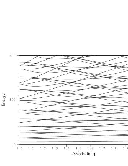
Figure 6: Single-particle spectra (in unit of $\varepsilon_{0}$) for the elliptic billiard plotted as functions of the deformation parameter $\eta$.

In Fig. 6 the deformation dependence of the single-particle energies for the elliptic billiard is presented. At the circular limit, the familiar shell gaps are clearly observed, while different shell gaps start to develop at higher deformations. Below we identify the semiclassical origin of these shell structures at higher deformations.

7.2 Strutinsky’s smoothed level densities and shell energies

=fig07.ps

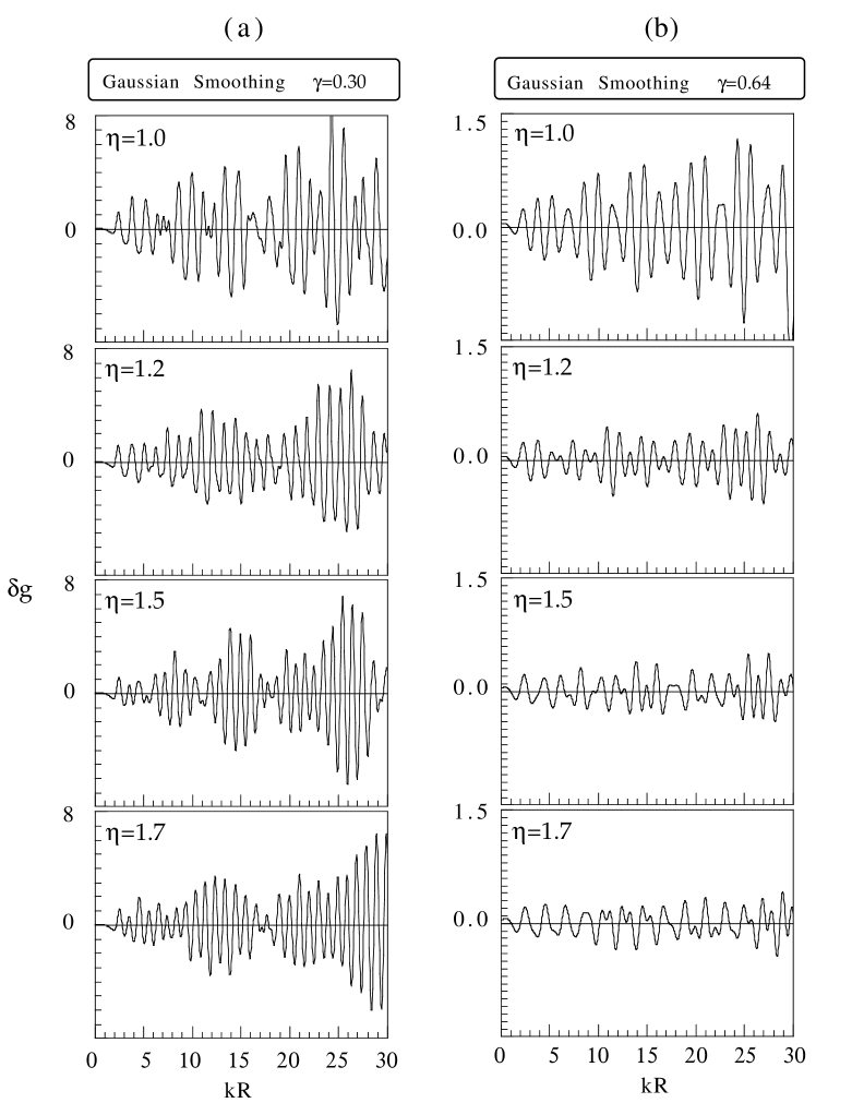
Figure 7: Coarse-grained level densities with the Gaussian smoothing parameter $\gamma=0.3$ (a) and 0.64 (b).

With the aid of the Strutinsky averaging procedure, [57] clear oscillatory patterns of the coarse-grained level density emerge as shown in Fig. 7, where (a) and (b) are obtained with the Gaussian smoothing parameter $\gamma$ (defined by (72)) of 0.30 and 0.64, respectively. As clearly seen from these figures, the choice of a Gaussian smoothing parameter $\gamma$ is rather crucial for properly identifying the coarse-grained level density, and hence the contribution of classical periodic orbits. At the circular limit $\eta=1.0$, both Gaussian-smoothed level densities show similar oscillations, whereas the shell gaps for $\gamma=0.64$ start to collapse with increasing deformation. In particular for deformations $\eta$ larger than 1.5 the strong shell patterns cease to exist for the case of $\gamma=0.64$, while for $\gamma=0.3$ the appreciable effects still remain and show more oscillations as deformation increases.

In the semiclassical picture, for a given value of $\gamma$ the contributions from only those periodic orbits of length up to $L_{\rm max}\approx\pi R/\gamma$ can be considered. In this context, it is important to locate the actual shell-energy minima, irrespective of the choice of a Gaussian smoothing parameter.

In terms of the particle number $N$ one can also obtain the shell-correction energy $\delta E$ defined as the difference between the sum of single-particle energies of $N$ lowest levels (taking the spin-degeneracy factor 2 into account) and the Strutinsky averaged energies, i.e.,

$$\delta E=\sum_{i=1}^{N}\varepsilon_{i}-\tilde{E},\qquad\tilde{E}=2\int_{-\infty}^{\tilde{\varepsilon}_{F}}d\varepsilon^{\prime}\,\varepsilon^{\prime}\,\tilde{g}(\varepsilon^{\prime}),$$ (77)

with the Fermi energy $\tilde{\varepsilon}_{F}$ satisfying

$$N=2\int_{-\infty}^{\tilde{\varepsilon}_{F}}d\varepsilon^{\prime}\,\tilde{g}(\varepsilon^{\prime}).$$ (78)

=fig08.ps

Figure 8: Shell structure energy $\delta E$ (in unit of $\varepsilon_{0}$) plotted as a function of both deformation $\eta$ and particle number $N$.

Figure 8 illustrates the oscillating pattern of the shell-correction energy $\delta E$ as function of both deformation $\eta$ and particle number $N$. It is clear from the figure that the distance between major shell gaps shrink with increasing deformation. In the considered range of deformation it is found that the actual magic numbers determined by the above procedure cannot be reproduced with the choice of $\gamma=0.64$, whereas the value of $\gamma=0.3$ is small enough not to demolish but still large enough to keep the actual coarse-grained shell structure. It is explicitly shown in Fig. 9, where the shell-correction energies are now calculated by applying a Gaussian smoothing parameters of $\gamma=0.3$ and 0.64, for the case of $\eta=1.5$ as an example.

=fig09.ps

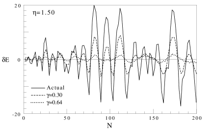
Figure 9: Smoothed shell-correction energies for $\eta=1.5$ with Gaussian smoothing parameter $\gamma=0.3$ (dashed line) and 0.6 (dotted line). Those without the smoothing are plotted by a solid line.

In this case, the actual magic numbers are found to be $\ldots,16,22,30,38,52,\ldots$, which exactly coincide with those of $\gamma=0.3$, while those calculated with $\gamma=0.64$ show larger oscillations missing $\ldots,16,30,\ldots$. The same is true for other deformations considered in this paper. So, the coarse-grained shell structure obtained with $\gamma=0.64$ is too rough and therefore we adapt $\gamma=0.3$ to improve the precision of its description.

7.3 Shell Structure and Fourier Spectra

Equations of single-particle motion in the billiard are invariant with respect to the scaling transformation $({\mathchoice{\mbox{\boldmath$\displaystyle r$}}{\mbox{\boldmath$\textstyle r$}}{\mbox{\boldmath$\scriptstyle r$}}{\mbox{\boldmath$\scriptstyle r$}}},{\mathchoice{\mbox{\boldmath$\displaystyle p$}}{\mbox{\boldmath$\textstyle p$}}{\mbox{\boldmath$\scriptstyle p$}}{\mbox{\boldmath$\scriptstyle p$}}},t)\to({\mathchoice{\mbox{\boldmath$\displaystyle r$}}{\mbox{\boldmath$\textstyle r$}}{\mbox{\boldmath$\scriptstyle r$}}{\mbox{\boldmath$\scriptstyle r$}}},\alpha{\mathchoice{\mbox{\boldmath$\displaystyle p$}}{\mbox{\boldmath$\textstyle p$}}{\mbox{\boldmath$\scriptstyle p$}}{\mbox{\boldmath$\scriptstyle p$}}},\alpha^{-1}t)$. The action integral $S_{\beta}$ for a periodic orbit $\beta$ is proportional to its length $L_{\beta}$,

$$S_{\beta}(E=p^{2}/2m)=\oint_{\beta}d{\mathchoice{\mbox{\boldmath$\displaystyle r$}}{\mbox{\boldmath$\textstyle r$}}{\mbox{\boldmath$\scriptstyle r$}}{\mbox{\boldmath$\scriptstyle r$}}}\cdot{\mathchoice{\mbox{\boldmath$\displaystyle p$}}{\mbox{\boldmath$\textstyle p$}}{\mbox{\boldmath$\scriptstyle p$}}{\mbox{\boldmath$\scriptstyle p$}}}=pL_{\beta}=\hbar kL_{\beta}.$$ (79)

and the semiclassical trace formula for the level density is written as

$$g_{\rm scl}(\varepsilon)=\tilde{g}(\varepsilon)+\sum_{\beta}A_{\beta}(kR)\cos\left(kL_{\beta}-\frac{\pi}{2}\mu_{\beta}\right)$$ (80)

where $\tilde{g}(\varepsilon)$ denotes the smooth part corresponding to the contribution of zero-length orbits, $A_{\beta}=\left|{\cal A}_{\beta}\right|$, $\mu_{\beta}$ the Maslov phase (the deformation and energy dependent phase of Eqs. (41) and (56) in our improved semiclassical approximation). As previously discussed, the stationary phase approximation employed in deriving the Gutzwiller trace formula breaks down at bifurcation points for stable periodic orbits, and consequently results in the divergence of the amplitudes $A_{\beta}(kR)$ in Eq. (80), whereas in the present ISP treatment those amplitudes are smooth functions of both deformation and energy.

In order to examine the classical-quantum correspondence on shell structure, one can perform the Fourier transform $F(L)$ of the quantum level density $g(\varepsilon)$ with respect to the wave number $k$

$$F(L)=\int dk\,e^{-ikL}g(\varepsilon)e^{-\frac{1}{2}\left(\frac{k}{k_{c}}\right)^{2}}=\frac{1}{2\varepsilon_{0}R^{2}}\sum_{i}\frac{1}{k_{i}}e^{-ik_{i}L}e^{-\frac{1}{2}\left(\frac{k_{i}}{k_{c}}\right)^{2}},$$ (81)

which may be regarded as ‘length spectrum’ exhibiting peaks at lengths of individual periodic orbits. Here the Gaussian factor is imposed to smoothly cutoff the spectrum in the high-energy region. In numerical calculations, we use $k_{c}=k_{\rm max}/\sqrt{2}$, $k_{\rm max}$ being the maximum wave number included. The above method of taking Fourier transform of the quantum level density is known to be a powerful tool to investigate the role of classical periodic orbits in the appearance of shell fluctuations in quantum systems, and from such observations one can also extract the semiclassical contributions of individual periodic orbits.

=fig10.ps

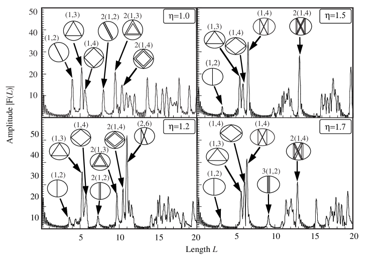
Figure 10: Fourier transforms of the single-particle level density for the elliptic billiards with $\eta=1.0$ (a), 1.2 (b), 1.5 (c) and 1.7 (d). Some periodic orbits that correspond to peaks are illustrated.

Fourier spectra for deformations $\eta=1.0$, 1.2, 1.5 and 1.7 are presented in Figs. 10(a), (b), (c) and (d), respectively. At axis ratio $\eta=1.0$, the diameter and elliptic orbits are found to be equally important. The fact that only those shorter periodic orbits mainly contribute to the gross-shell structure implies the significance of three classical periodic orbits at the circular limit, namely the diameter, triangular, and square shape orbits. As deformation increases, the Fourier amplitudes for triangular and rhombic orbits still exhibit fairly strong effects, while those for diameter orbits start to decline quickly and significant rearrangement can be observed. Especially at deformations $\eta=1.5$ and 1.7, one can conclude, in addition to triangular and rhombic shape orbits, the gross-shell fluctuations are also governed by the (1,4) hyperbolic orbits bifurcated from the 2(1,2) short diameter orbit at the critical deformation $\eta=\sqrt{2}$.

=fig11.ps

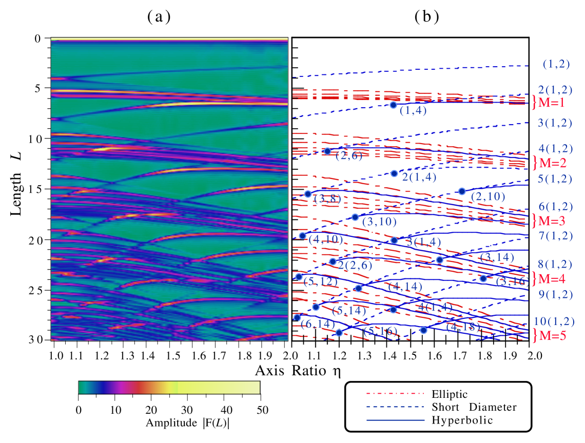
Figure 11: (a) Modulus of the Fourier amplitudes plotted as functions of both orbit-length $L$ and deformation $\eta$. (b) Lengths $L$ of classical periodic orbits calculated as function of deformation $\eta$. Solid, dashed and dash-dotted lines are used for hyperbolic, short-diameter, and elliptic orbits, respectively.

Figure 11(a) demonstrates the deformation dependence of Fourier amplitudes calculated from the quantum single-particle spectra. Here the enhancement of peaks indicates a larger contribution from the corresponding classical periodic orbits $\beta$ of length $L_{\beta}$ to the shell structure. At the circular limit the system possesses the highest symmetry, and the breaking of this symmetry due to a small deviation of its shape results in the orbital bifurcation. With increasing deformation, the short diameter orbits with $M$ repetitions $M$(1,2) also bifurcate and create hyperbolic orbits at the critical deformations $\eta_{\rm bif}$ given by Eq. (18). The length of those classical periodic orbits as a function of deformation can be calculated [14] as shown in Fig. 11(b). It is clearly seen from both figures that the bifurcations of stable periodic orbits give rise to an increase in the Fourier amplitudes. The remarkable enhancements seen in the figure exactly coincide with the corresponding lengths of the newly created hyperbolic orbits, and hence stress the importance of the orbital bifurcations.

In this context, similar enhancements for the case of a spheroidal cavity at superdeformed shape were also reported in Ref. [21], where superdeformed shell structure is associated with bifurcations of periodic orbits with two repetitions on the equatorial plane. In the present work, particular attention is paid to investigate such correlations between bifurcations of stable periodic orbits and quantum level-density oscillations.

=fig12.ps

Figure 12: Deformation dependence of Fourier peak heights for hyperbolic and short diametric orbits 2(1,2), (1,4), 3(1,2), (1,6), 4(1,2) and (1,8). Solid lines are used for multiple traversals along the short diameter, $M$(1,2) with $M=1,2,3$, while long-dashed, short-dashed and dotted lines are used for hyperbolic (1,4),(1,6),(1,8) orbits, respectively. Open circles indicate the bifurcation points.

In Fig. 12, Fourier peak heights for some of the important hyperbolic orbits, namely those bifurcated from the short diameter orbits of 2, 3, and 4 repetitions, 2(1,2), 3(1,2) and 4(1,2), are displayed as a function of deformation $\eta$. Interestingly, the Fourier peaks for these newly created orbits show a rather universal deformation dependence, that is, their heights reach the maxima shortly after their bifurcation points and quickly decrease with increasing deformation. Such remarkable features were already seen in Fig. 8, where the shell valleys for $\eta$ approximately larger than 1.5 can be understood to vary along the constant-action lines $S(k,\eta)=\mbox{const.}$ of the (1,4) hyperbolic orbits, as explained below.

Suppose some classical periodic orbits $\beta$ of length $L_{\beta}$ are the dominant components in the semiclassical trace formula for the oscillating level density, then the shell valley maxima/minima follows the constant-action lines $S_{\beta}(k,\eta)=\mbox{const.}$ of those dominating classical periodic trajectories. Referring to Eq. (80), such lines are determined by

$$kL_{\beta}-\frac{\pi}{2}\mu_{\beta}=(2n+1)\pi,\qquad n=0,1,2,\ldots$$ (82)

=fig13.ps

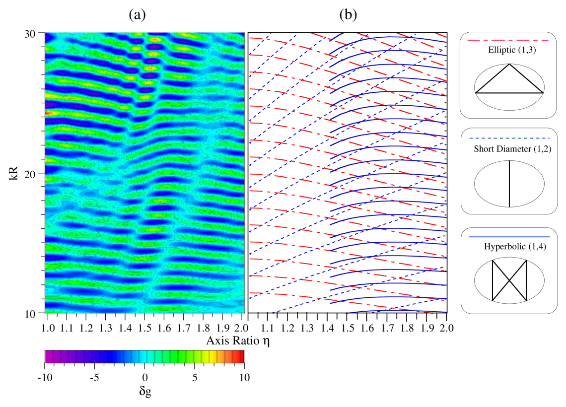
Figure 13: (a) Smoothed level density plotted on the $k$-$\eta$ plane. (b) Constant action lines on the $k$-$\eta$ plane for the elliptic $(1,3)$ orbit (dash-dotted lines), the primitive short diameter $1(1,2)$ orbit (short-dashed lines) and the hyperbolic $(1,4)$ orbit (solid lines).

We shall now demonstrate the above dependence in Fig. 13(a), where the smoothed level densities are plotted on the $k$-$\eta$ plane. As indicated in Fig. 13(b), it is interesting to note that the shell valley structures seen in Fig. 13(a) can be described by the constant-action lines of three major periodic orbits; near the circular limit the shell valleys vary along those of elliptic (mainly triangular and rhombic) orbits; in the right-half region of Fig. 13(a) the influence of newly created (1,4) hyperbolic orbits is visible; the contribution of short diameter orbits are less pronounced but certainly non-negligible throughout the considered range of deformation. The equality, Eq. (82), indicates the inverse proportionality relation between the orbital length $L_{\beta}$ and wave number $k$. As the length of a trajectory $\beta$ increases, the values of $k$ decrease and consequently the smoothed level densities show more oscillations. In particular, since the length of the (1,4) hyperbolic orbits gradually increases within $\eta\approx\sqrt{2}-1.7$ and then slowly decreases for $\eta>1.7$, the corresponding constant-action lines also behave in the same manner. Such a tendency was already observed in Fig. 8, where the contribution from the (1,4) hyperbolic orbits to the shell energy $\delta E$ is apparent in the region $\eta>1.5$, indicating the essential role of the orbital bifurcations in quantal shell formations.

8 Comparison between Quantum and Semiclassical Calculations

=fig14a.ps

Figure 14: (a) Amplitude modulus $A$ for bifurcating short diameter $2(1,2)$ and butterfly $1(1,4)$ orbits obtained by ISPM are shown by solid lines as functions of deformation parameter $\eta$; standard results of the extended Gutzwiller periodic orbit theory (SSPM) are shown by short-dashed lines. (b) ISPM amplitudes for the butterfly orbit (solid line) are compared with exact calculation of the Poisson-sum trace formula (27) (dashed line marked by “Poisson”) and SSPM of Berry and Tabor [4] (dotted line).

=fig15a.ps

Figure 15: (a) Same as in Fig. 14(a) but for primitive short diameter $1(1,2)$ and triangle $1(1,3)$ orbits for smaller deformations. (b) Comparison of the amplitudes for 1(1,3) with exact calculations and SSPM. Notations are the same as in Fig. 14(b).

Figures 14,15,16 show the modulus of the complex amplitude for a few short orbits. The semiclassical amplitudes for the hyperbolic “butterfly” $M(n_{u},n_{v})=(1,4)$ and elliptic triangular (1,3) orbit families calculated by the ISPM are in good agreement with the exact calculation of the Poisson-sum trace integral (22), see Figs. 14 and 15, respectively. All ISPM amplitudes are continuous function of the deformation through the bifurcation point $\eta=\sqrt{2}$. A remarkable enhancement of the butterfly amplitude is seen at the deformation $\eta=1.5\mbox{--}1.6$ slightly on the right of the bifurcation point (see Fig. 14).

The ISPM amplitude for the primitive short diameter 1(1,2) quickly approaches the Gutzwiller SSPM result as one goes away from the circular limit and, for larger deformations, its magnitude is relatively small compared with those of other orbits mentioned above (see Fig. 15).

=fig16.ps

Figure 16: ISPM amplitude modulus (solid line) for the sum of short and long diameter $2(1,2)$ orbits is compared with the ($n_{u}=1,n_{v}=2,M=2$) part of the Poisson-sum trace formula (27) (long-dashed line) and the Gutzwiller SSPM (dotted line).

In Fig. 16 we compare the ISPM result with the modulus of “diametric” part of the Poisson-sum trace formula corresponding to $n_{u}=1$, $n_{v}=2$ and $M=2$, which is regarded in Ref. [24] as to represent short and long diameters, as well as the standard Gutzwiller results. The ISPM amplitude for the bifurcating short diameter 2(1,2) has the two maxima; at the bifurcation deformation $\sqrt{2}$, which is significantly larger than the butterfly and triangular amplitudes, and at the circular shape, see also Figs. 14 and 15. (Similar maxima at the circular shape appear for any short diameter orbit. The maximum for the short diameter 1(1,2) is the largest one, in particular, larger than for the triangular orbit, see Fig. 15(a).) As seen from Fig. 16, there is the same circular shape limit for the ISPM approach and the “diametric” part of the Poisson-sum trace formula, which is identical to the diameter family amplitude in the circular disk.

Apparently, the behaviour of the ISPM amplitude for two repetitions of the short diameter 2(1,2) is essentially different from that of the “diametric” part of the Poisson-sum trace integral which exhibits no enhancement near the bifurcation point. Thus, the Poisson-sum trace formula (27) describes the families with maximum degeneracy like hyperbolic and elliptic orbits, rather than the isolated diameters. For the isolated orbits with smaller degeneracy like diameters in elliptic billiard the Poisson-sum trace formula cannot be applied because of the isolated stationary points for the angle $\Theta_{u}$ variable. This is the reason for the agreement of the ISPM and SSPM asymptotics unlike for the “diametric” term of the Poisson-sum trace integral in Eq.(27). It means that the diameters cannot be included in the usual EBK rational torus quantization. However, the diameters could be included in a more general quantization rule in terms of the averaged ISPM level densities (66) in a similar way as pointed out in Refs. [9, 12].

We note a significant improvement of the ISPM results compared to the SSPM for $\sigma$ close to the separatrix value $1$ and the creeping value $\sigma_{\rm cr}$ (17). These cases might seem to be important only in the limit $\eta\rightarrow\infty$ when $\sigma_{\rm cr}$ tends to unity. However, even for $0\leq\eta\mathop{\vbox{\offinterlineskip\hbox{$<$}\hbox to7.7778pt{\hss\hbox{$\sim$}\hss}}}2$ we meet the situations where the stationary points are close to the critical points $\sigma=1$ and $\sigma=\sigma_{\rm cr}$, so that we have to integrate within the finite limits.

=fig17a.ps

Figure 17: Quantum and semiclassical (ISPM) oscillating level densities $\delta g(kR)$ versus $kR$ for several deformations. Averaging parameter $\gamma=0.3$, parameter of the Strutinsky’s shell correction method $\tilde{\gamma}=2.0$ and correction polynomial degree $2{\cal M}=6$ are used.

We compare in Fig. 17 the semiclassical level densities $\delta g_{\rm scl}(kR)$ calculated by the ISPM with the quantum results for the averaging parameter $\gamma=0.3$. The results obtained by the ISPM are in good agreement with quantum results even near the bifurcation point $\sqrt{2}$, where the SSPM gives the divergent result due to the zeros of the stability factor $F_{sM}$ for the short diameters 2(1,2). For the deformations like $1.2$ and $1.7$ far from the bifurcation, one obtains a fair agreement between the ISPM and the SSPM.

=fig18a.ps

Figure 18: Oscillating level density $\delta g(kR)$ versus $kR$ (left-hand side) and shell energy $\delta E$ in units $\varepsilon_{0}$ versus $N^{1/2}$ (right-hand side) for a small deformation 1.01. Solid and dotted lines indicate results of quantum and ISPM calculations, respectively. Parameters of the Strutinsky’s shell correction method are the same as in Fig. 17.

=fig19.ps

Figure 19: Quantum and ISPM shell energy $\delta E$ (in unit of $\varepsilon_{0}$) are plotted by solid and dotted lines, respectively, as functions of $N^{1/2}$.

Figure 19 shows a nice convergence of the ISPM results to those of the circular disk trace formula for $\eta\to 1$. This convergence is seen for any small deformation when the semiclassical parameter $kR$ becomes sufficiently large. With the inclusion of the closed (periodic and non-periodic) hyperbolic orbit contribution, one gets even better agreement with the quantum densities near the circular disk shape. For deformations far from the circular shape ($\eta\mathop{\vbox{\offinterlineskip\hbox{$>$}\hbox to7.7778pt{\hss\hbox{$\sim$}\hss}}}1.1$) and far from other bifurcation points, the contribution of the hyperbolic “co2” orbits approaches Gutzwiller’s SSPM result for the isolated diameters, see Fig. 5(b).

For the averaging parameter $\gamma=0.64$, we have good convergence of POT sums for the ISPM and SSPM with a few short periodic orbits with $M\leq 1$, $n_{u}=1$ and $n_{v}\leq 10$. This is due to the damping factor in Eq. (73) which ensures the convergence of the POT sum. For smaller $\gamma=0.3$ we need more orbits with $M\leq 2$, $n_{u}\leq 2$ and $n_{v}\leq 10$. Note that for $\gamma=0.3$ we have much better agreement of the ISPM results with quantum mechanical calculations than in the case of SSPM for the deformations near the bifurcations including the transition to the circular shape, see Fig. 7.

=fig20.ps

Figure 20: Shell energy maps $\delta E$ drawn as function of $N^{1/2}$ and deformation $\eta$. (Left-hand side) Quantum results like in Figs. 16, 19 and 19: (Middle- and right-hand sides) Semiclassical ISPM results with and without taking into account the bifurcating orbits, respectively (see text).

Figures 19 and 20 show nice agreements of the ISPM results for the shell-correction energies with the corresponding quantum results. Note that we substitute the exact Fermi energy $\varepsilon_{F}$ into the semiclassical shell energy $\delta E$ (67) by using the second equation for the particle number there and quantum level density like in Ref. [11]. This is important to get the correct behaviour of the shell-correction energy as a function of particle number $N$, as explained in Ref. [11]. It is evident from Fig. 20 that the nice agreement between the ISPM and quantum results in the strongly deformed region of $\eta\geq\sqrt{2}$ cannot be attained without including the contributions from bifurcating 2(1,2) and (1,4) orbits.

In all our calculations we used the semiclassical approximation improved at the bifurcation points which becomes better with increasing $kR$ for all deformations including the bifurcation points.

9 Conclusion

The most essential new result of this paper in comparison to the Berry-Tabor theory are two additional terms (second and third ones in Eq. (66)) in the improved trace formula for the elliptic billiard. These two terms represent the contributions from the short and long diameters which are continuous functions through all bifurcation points. For deformations far from the bifurcation points, we obtain asymptotically the standard Gutzwiller result for the isolated diameters, and the correct trace formula for the diameters in spherical limit of the circular billiard. Our results for the hyperbolic and elliptic orbits improved near the bifurcation points are simpler than those suggested within the uniform approximation [4, 26].

With the use of our improved trace formula, we have demonstrated the importance of bifurcations of the repeated short diameter orbit for the emergence of shell structure at large deformations.

Appendices

Appendix A Curvatures

The actions $I_{u}$ and $I_{v}$ given by Eq. (11) are expressed explicitly in terms of the elliptic integrals [47, 49]. For elliptic orbits one has

$$I_{u} = \frac{2}{\pi}\zeta\sqrt{2m\varepsilon\sigma}\,\mathop{\rm E}\left(\frac{\pi}{2},\frac{1}{\sqrt{\sigma}}\right),$$

$$I_{v} = \frac{1}{\pi}\zeta\sqrt{2m\varepsilon\sigma}\left[\mathop{\rm E}\left(\theta_{e},\frac{1}{\sqrt{\sigma}}\right)-\mathop{\rm E}\left(\frac{\pi}{2},\frac{1}{\sqrt{\sigma}}\right)+\frac{\eta^{2}-\sigma(\eta^{2}-1)}{\eta\sqrt{\eta^{2}-1}}\right].$$ (83)

For hyperbolic orbits,

$$I_{u} = \frac{2}{\pi}\zeta\sqrt{2m\varepsilon}\left[\mathop{\rm E}\left(\frac{\pi}{2},\frac{1}{\sqrt{\sigma}}\right)-(1-\sigma)\mathop{\rm F}\left(\frac{\pi}{2},\frac{1}{\sqrt{\sigma}}\right)\right],$$

$$I_{v} = \frac{1}{\pi}\zeta\sqrt{2m\varepsilon}\left\{(1-\sigma)\left[\mathop{\rm F}\left(\frac{\pi}{2},\frac{1}{\sqrt{\sigma}}\right)-\mathop{\rm F}\left(\theta_{h},\frac{1}{\sqrt{\sigma}}\right)\right]\right.$$ (84)

$$\qquad\left.+\mathop{\rm E}\left(\theta_{h},\frac{1}{\sqrt{\sigma}}\right)-\mathop{\rm E}\left(\frac{\pi}{2},\frac{1}{\sqrt{\sigma}}\right)+\frac{\eta^{2}-\sigma(\eta^{2}-1)}{\eta\sqrt{\eta^{2}-1}}\right\}$$

Eqs. (83) and (84) may be regarded as equations for the energy surface $\varepsilon(I_{u},I_{v})$ written in terms of the parameter $\sigma$ for its elliptic and hyperbolic parts, respectively.

The curvature $K$ of the energy curve are obtained by differentiating Eqs. (83) and (84) with respect to the parameter $\sigma$. In this way one gets Eq. (19) with the following derivatives for elliptic orbits,

$$\frac{\partial I_{u}}{\partial\sigma} = \frac{1}{\pi}\frac{\zeta\sqrt{2m\varepsilon}}{\sqrt{\sigma}}\mathop{\rm F}\left(\frac{\pi}{2},\frac{1}{\sqrt{\sigma}}\right),$$

$$\frac{\partial^{2}I_{u}}{\partial\sigma^{2}} = -\frac{1}{2\pi}\frac{\zeta\sqrt{2m\varepsilon}}{\sqrt{\sigma^{3}}}\Pi\left(\frac{\pi}{2},\frac{1}{\sigma},\frac{1}{\sqrt{\sigma}}\right),$$

$$\frac{\partial I_{v}}{\partial\sigma} = -\frac{1}{2\pi}\frac{\zeta\sqrt{2m\varepsilon}}{\sqrt{\sigma}}\left[\mathop{\rm F}\left(\frac{\pi}{2},\frac{1}{\sqrt{\sigma}}\right)-\mathop{\rm F}\left(\theta_{e},\frac{1}{\sqrt{\sigma}}\right)\right],$$

$$\frac{\partial^{2}I_{v}}{\partial\sigma^{2}} = \frac{1}{4\pi}\frac{\zeta\sqrt{2m\varepsilon}}{\sqrt{\sigma^{3}}}\left[\Pi\left(\frac{\pi}{2},\frac{1}{\sigma},\frac{1}{\sqrt{\sigma}}\right)-\Pi\left(\theta_{e},\frac{1}{\sigma},\frac{1}{\sqrt{\sigma}}\right)+\frac{\eta\sqrt{\eta^{2}-1}}{\sqrt{1-(1-\sigma^{-1})\eta^{2}}}\right].$$

For hyperbolic orbits,

$$\frac{\partial I_{u}}{\partial\sigma} = \frac{1}{\pi}\zeta\sqrt{2m\varepsilon}\mathop{\rm F}\left(\frac{\pi}{2},\sqrt{\sigma}\right),$$

$$\frac{\partial^{2}I_{u}}{\partial\sigma^{2}} = \frac{1}{2\pi}\frac{\zeta\sqrt{2m\varepsilon}}{\sigma}\left[\Pi\left(\frac{\pi}{2},\sigma,\sqrt{\sigma}\right)-\mathop{\rm F}\left(\frac{\pi}{2},\sqrt{\sigma}\right)\right],$$

$$\frac{\partial I_{v}}{\partial\sigma} = \frac{1}{2\pi}\zeta\sqrt{2m\varepsilon}\left[\mathop{\rm F}\left(\theta_{h},\sqrt{\sigma}\right)-\mathop{\rm F}\left(\frac{\pi}{2},\sqrt{\sigma}\right)\right],$$

$$\frac{\partial^{2}I_{v}}{\partial\sigma^{2}} = \frac{1}{4\pi}\frac{\zeta\sqrt{2m\varepsilon}}{\sigma}\left[\Pi\left(\theta_{h},\sigma,\sqrt{\sigma}\right)-\Pi\left(\frac{\pi}{2},\sigma,\sqrt{\sigma}\right)+\mathop{\rm F}\left(\frac{\pi}{2},\sqrt{\sigma}\right)-\mathop{\rm F}\left(\theta_{h},\sqrt{\sigma}\right)\right].$$ (86)

With Eq. (LABEL:derivate) we obtain the curvature $K_{\beta}$ (19) for elliptic orbits as

$$K_{\beta}=\frac{\pi}{4p\zeta}\frac{\kappa}{\mathop{\rm F}^{2}(\frac{\pi}{2},\kappa)}\left[\frac{\mathop{\rm F}(\theta,\kappa)}{\mathop{\rm F}(\frac{\pi}{2},\kappa)}\Pi\left(\frac{\pi}{2},\kappa^{2},\kappa\right)-\Pi(\theta,\kappa^{2},\kappa)+\frac{\eta\sqrt{\eta^{2}-1}}{\sqrt{1-(1-\kappa^{2})\eta^{2}}}\right].$$

(87)

For hyperbolic orbits,

$$K_{\beta}=\frac{\pi}{4p\zeta}\frac{1}{\kappa^{2}\mathop{\rm F}^{2}(\frac{\pi}{2},\kappa)}\left[\Pi(\theta,\kappa^{2},\kappa)-\frac{\mathop{\rm F}(\theta,\kappa)}{\mathop{\rm F}(\frac{\pi}{2},\kappa)}\Pi\left(\frac{\pi}{2},\kappa^{2},\kappa\right)\right].$$ (88)

Appendix B Separatrix

Like for the case of turning points [39, 40, 41, 42] one writes

$$\frac{1}{\hbar}\left[S_{\alpha}(\mathchoice{\mbox{\boldmath$\displaystyle I$}}{\mbox{\boldmath$\textstyle I$}}{\mbox{\boldmath$\scriptstyle I$}}{\mbox{\boldmath$\scriptstyle I$}}^{\prime},\mathchoice{\mbox{\boldmath$\displaystyle I$}}{\mbox{\boldmath$\textstyle I$}}{\mbox{\boldmath$\scriptstyle I$}}{\mbox{\boldmath$\scriptstyle I$}}^{\prime\prime},t_{\alpha})-(\mathchoice{\mbox{\boldmath$\displaystyle I$}}{\mbox{\boldmath$\textstyle I$}}{\mbox{\boldmath$\scriptstyle I$}}{\mbox{\boldmath$\scriptstyle I$}}^{\prime\prime}-\mathchoice{\mbox{\boldmath$\displaystyle I$}}{\mbox{\boldmath$\textstyle I$}}{\mbox{\boldmath$\scriptstyle I$}}{\mbox{\boldmath$\scriptstyle I$}}^{\prime})\cdot\mathchoice{\mbox{\boldmath$\displaystyle\Theta$}}{\mbox{\boldmath$\textstyle\Theta$}}{\mbox{\boldmath$\scriptstyle\Theta$}}{\mbox{\boldmath$\scriptstyle\Theta$}}^{\prime\prime}\right] = c_{0}^{\parallel}+c_{1}^{\parallel}x+c_{2}^{\parallel}x^{2}+c_{3}^{\parallel}x^{3}+\ldots$$ (89)

$$\equiv \tau_{0}^{\parallel}+\tau_{1}^{\parallel}z+\frac{1}{3}z^{3}.$$

Here,

$$x=(I_{u}^{\prime}-{I_{u}^{\prime}}^{*})/\hbar,$$ (90)

$$c_{0}^{\parallel} = \frac{1}{\hbar}\left[S_{\alpha}^{*}(\mathchoice{\mbox{\boldmath$\displaystyle I$}}{\mbox{\boldmath$\textstyle I$}}{\mbox{\boldmath$\scriptstyle I$}}{\mbox{\boldmath$\scriptstyle I$}}^{\prime},\mathchoice{\mbox{\boldmath$\displaystyle I$}}{\mbox{\boldmath$\textstyle I$}}{\mbox{\boldmath$\scriptstyle I$}}{\mbox{\boldmath$\scriptstyle I$}}^{\prime\prime},t_{\alpha})-(\mathchoice{\mbox{\boldmath$\displaystyle I$}}{\mbox{\boldmath$\textstyle I$}}{\mbox{\boldmath$\scriptstyle I$}}{\mbox{\boldmath$\scriptstyle I$}}^{\prime}-\mathchoice{\mbox{\boldmath$\displaystyle I$}}{\mbox{\boldmath$\textstyle I$}}{\mbox{\boldmath$\scriptstyle I$}}{\mbox{\boldmath$\scriptstyle I$}}^{\prime\prime})^{*}\cdot{\mathchoice{\mbox{\boldmath$\displaystyle\Theta$}}{\mbox{\boldmath$\textstyle\Theta$}}{\mbox{\boldmath$\scriptstyle\Theta$}}{\mbox{\boldmath$\scriptstyle\Theta$}}^{\prime\prime}}^{*}\right]=\frac{1}{\hbar}S_{\alpha}^{*}(\mathchoice{\mbox{\boldmath$\displaystyle\Theta$}}{\mbox{\boldmath$\textstyle\Theta$}}{\mbox{\boldmath$\scriptstyle\Theta$}}{\mbox{\boldmath$\scriptstyle\Theta$}}^{\prime},\mathchoice{\mbox{\boldmath$\displaystyle\Theta$}}{\mbox{\boldmath$\textstyle\Theta$}}{\mbox{\boldmath$\scriptstyle\Theta$}}{\mbox{\boldmath$\scriptstyle\Theta$}}^{\prime\prime},\varepsilon),$$ (91)

$$c_{1}^{\parallel} = \left(\frac{\partial S_{\alpha}}{\partial I_{u}^{\prime}}-\Theta_{u}^{\prime\prime}\right)^{*}=\Theta_{u}^{\prime}-\Theta_{u}^{\prime\prime}\to 0,\qquad(\sigma\to 1)$$ (92)

$$c_{2}^{\parallel} = \frac{\hbar}{2}\left(\frac{\partial^{2}S_{\alpha}}{\partial{I_{u}^{\prime}}^{2}}\right)^{*}=2\pi M\hbar K^{\parallel}\to\infty,\qquad(\sigma\to 1)$$ (93)

$$c_{3}^{\parallel} = \frac{\hbar^{2}}{6}\left(\frac{\partial^{3}S_{\alpha}}{\partial{I_{u}^{\prime}}^{3}}\right)^{*}=\frac{2\pi\hbar^{2}M}{3}\left(\frac{\partial K^{\parallel}}{\partial I_{u}}\right)<0,\qquad(\sigma\to 1)$$ (94)

where the star means $I_{u}^{\prime}=I_{u}^{\prime\prime}=I_{u}^{*}$. The asymptotic behaviour of the constants $c_{i}^{\parallel}$ near the separatrix $\sigma\approx 1$ was found from

$$K^{\parallel}\to\frac{\pi\log[(1+\sin\theta)/(1-\sin\theta)]}{p\zeta(\sigma-1)\log^{3}(\sigma-1)},\qquad(\sigma\to 1)$$ (95)

$\theta\to\theta_{h}(\eta)$ formally, see (15),

$$\frac{\partial K^{\parallel}}{\partial I_{u}}\to-\frac{2\pi^{2}\log[(1+\sin\theta)/(1-\sin\theta)]}{(p\zeta(\sigma-1)\log^{2}(\sigma-1))^{2}}.\qquad(\sigma\to 1)$$ (96)

The second equality in Eq. (89) was obtained by a linear transformation with some constants $\alpha$ and $\beta$,

$$x=\alpha z+\beta,\qquad\alpha=(3c_{3}^{\parallel})^{-1/3},\qquad\beta=-c_{2}^{\parallel}/(3c_{3}^{\parallel}),$$ (97)

$$\tau_{0}^{\parallel}=(c_{0}-c_{1}c_{2}/(3c_{3})+2c_{2}^{3}/(27c_{3}^{2}))^{\parallel},\qquad\tau_{1}^{\parallel}=\alpha[c_{1}-c_{2}^{2}/(3c_{3})]^{\parallel}.$$ (98)

Near the stationary point for $\sigma\to 1$, one has $c_{1}^{\parallel}\to 0$ and $\tau_{1}^{\parallel}\to-w_{\parallel}$ with the positive quantity

$$w_{\parallel}=\left({c_{2}^{2}\over{(3c_{3})^{4/3}}}\right)^{\parallel}\to\left|\frac{M\log[(1+\sin\theta)/(1-\sin\theta)]p\zeta(\sigma-1)}{2\hbar\log(\sigma-1)}\right|^{2/3}.$$ (99)

Using expansion (89) in Eq. (21) and taking the integral over angle $\Theta_{v}^{\prime\prime}$ exactly, i.e. writing $2\pi$ instead of this integral, one gets

$$\delta g_{\rm scl}^{(lM)} = -\frac{2}{\hbar}\mathop{\rm Re}\sum_{\alpha}\int d\Theta_{u}^{\prime\prime}\frac{1}{\left|\omega_{v}^{*}\right|}e^{i(\tau_{0}-\nu_{\alpha})}\sqrt{\frac{\sqrt{w_{\parallel}}}{c_{2}^{\parallel}}}$$

$$\times\left[\mathop{\rm Ai}\left(-w_{\parallel},{\cal Z}_{lM,1}^{\parallel},{\cal Z}_{lM,2}^{\parallel}\right)+i\mathop{\rm Gi}\left(-w_{\parallel},{\cal Z}_{lM,1}^{\parallel},{\cal Z}_{lM,2}^{\parallel}\right)\right]$$

$$\approx -\frac{2}{\hbar}\mathop{\rm Re}\sum_{\alpha}\int d\Theta_{u}^{\prime\prime}\frac{1}{\left|\omega_{v}^{*}\right|}e^{i(\tau_{0}-\nu_{\alpha})}\sqrt{\frac{\sqrt{w_{\parallel}}}{c_{2}^{\parallel}}}\left[\mathop{\rm Ai}\left(-w_{\parallel}\right)+i\mathop{\rm Gi}\left(-w_{\parallel}\right)\right],$$

where

$${\cal Z}_{lM,1}^{\parallel}=\sqrt{w_{\parallel}},\qquad{\cal Z}_{lM,2}^{\parallel}=\sqrt{\frac{c_{2}^{\parallel}}{\sqrt{w_{\parallel}}}}\,\frac{I_{u}^{\rm(cr)}}{\hbar}+\sqrt{w_{\parallel}}.$$ (101)

$\mathop{\rm Ai}(-w,z_{1},z_{2})$ and $\mathop{\rm Gi}(-w,z_{1},z_{2})$ are incomplete Airy and Gairy functions, [48]

$$\left\{\begin{array}[]{c}\mathop{\rm Ai}(-w,z_{1},z_{2})\\ \mathop{\rm Gi}(-w,z_{1},z_{2})\end{array}\right\}=\frac{1}{\pi}\int_{z_{1}}^{z_{2}}dz\,\left\{\begin{array}[]{c}\cos\\ \sin\end{array}\right\}\left(-wz+z^{3}/3\right),$$ (102)

and $\mathop{\rm Ai}(-w)$ and $\mathop{\rm Gi}(-w)$ are the corresponding standard complete functions [47]. We used in the second equation of Eq. (LABEL:pstracelang) that for any finite deformation $\eta$ and large $kR$ near the separatrix ($\sigma\to 1$) one gets (see Eq. (99))

$${\cal Z}_{lM,1}^{\parallel}\to 0,\quad{\cal Z}_{lM,2}^{\parallel}\to 4\left[\frac{M\log[(1+\sin\theta)/(1-\sin\theta)]p\zeta}{2(\sigma-1)^{2}\log^{4}(\sigma-1)}\right]^{1/3}$$

$$\times\left[\frac{\eta}{\sqrt{\eta^{2}-1}}\mathop{\rm E}\left(\frac{\pi}{2},\frac{\sqrt{\eta^{2}-1}}{\eta}\right)-1\right]\to\infty.$$ (103)

Using an analogous expansion of the action $\tau_{0}$ in Eq. (LABEL:pstracelang) with respect to the angle $\Theta_{u}^{\prime\prime}$ to the third order and making a linear transformation like Eq. (97), one arrives at Eq. (59). We introduced in (59) several new quantities like

$$w_{\perp}=\left(\frac{c_{2}^{2}}{(3c_{3})^{4/3}}\right)^{\perp}>0,$$ (104)

$${\cal Z}_{lM,2}^{\perp}=\sqrt{w_{\perp}},\qquad{\cal Z}_{lM,2}^{\perp}=\frac{\pi}{2}\left(\left|3c_{3}^{\perp}\right|\right)^{1/3}+\sqrt{w_{\perp}},$$ (105)

$$c_{2}^{\perp}=\frac{1}{2\hbar}(J_{\alpha}^{\perp})^{*}=\frac{1}{2\hbar}\left(\frac{\partial^{2}S_{\alpha}}{\partial{\Theta_{u}^{\prime}}^{2}}+2\frac{\partial^{2}S_{\alpha}}{\partial\Theta_{u}^{\prime}\partial\Theta_{u}^{\prime\prime}}+\frac{\partial^{2}S_{\alpha}}{\partial{\Theta_{u}^{\prime\prime}}^{2}}\right)_{lM}^{*}=-\frac{F_{lM}}{8\pi MK^{\parallel}},$$ (106)

where $F_{lM}$ is the stability factor for long diameters, see Eq. (61),

$$c_{3}^{\perp} = \frac{1}{6\hbar}\left[\frac{\partial^{3}S_{\alpha}}{\partial{\Theta_{u}^{\prime}}^{3}}+3\frac{\partial^{3}S_{\alpha}}{\partial{\Theta_{u}^{\prime}}^{2}\partial\Theta_{u}^{\prime\prime}}+3\frac{\partial^{3}S_{\alpha}}{\partial\Theta_{u}^{\prime}\partial{\Theta_{u}^{\prime\prime}}^{2}}+\frac{\partial^{3}S_{\alpha}}{\partial{\Theta_{u}^{\prime\prime}}^{3}}\right]^{*}$$ (107)

$$= \frac{1}{6\hbar}\left[\frac{\partial J_{\alpha}^{\perp}}{\partial\Theta_{u}^{\prime}}+\frac{\partial J_{\alpha}^{\perp}}{\partial\Theta_{u}^{\prime\prime}}\right]^{*}<0.$$

Note, according to Eq. (106), the quantity $c_{2}^{\perp}$ goes to $0$ near the separatrix ($\sigma\to 1$) like for the caustic case. This is the reason why the Maslov-Fedoryuk theory [39, 40, 41, 42] can be used for the transformation of the integral over angle $\Theta_{u}^{\prime\prime}$ in Eqs. (LABEL:pstracelang) into Eq. (59).

Appendix C Jacobians for closed orbits with two reflection points

The Jacobian $J_{\rm co2}^{\parallel}$ defined by the derivative in Eq. (64) for closed orbits $\alpha$ like “co2” with two reflection points, $J_{\rm co2}^{\parallel}=\left(\delta{\bar{y}}^{\prime\prime}/\delta\theta_{p}^{\prime}\right)_{co2}$, can be calculated by means of the caustic method [11]. The main idea of this method is to use a specific property of the trajectories in billiard system like elliptic cavity. They are the straight lines which tangent a curve called the elliptic or hyperbolic caustics between turning points. Our trajectory stability problem for the variations $\delta{\bar{y}}^{\prime\prime}$ at a given $\delta\theta_{p}^{\prime}$, see Fig. 3, is much simplified by reducing it to the calculation of the caustics semi-axes $a_{c},b_{c}$ and $a_{c}+\delta a_{c},b_{c}+\delta b_{c}$ for closed orbit “co2” and its $\delta\theta_{p}^{\prime}$ deflection, respectively. For the case of closed non-periodic orbits “co2” the semi-axes $a_{c}$ and $b_{c}$ and their variations are functions of the initial point $(x,y)$ in contrast to the stability problem for the periodic orbits of Ref. [11]. The orbit-length invariant curve (confocal-to-boundary ellipse or hyperbola crossing the point $(x,y)$, see Fig. 4) and its semi-axis variations play a similar role for the calculation of the “co2” stability factor $J_{\rm co2}^{\parallel}$ with that of the boundary parameter for the periodic orbits in Ref. [11]. In this way this stability factor is obtained in the form

$$J_{\rm co2}^{\parallel}=\frac{q_{0}-q_{1}}{\sqrt{1+q_{1}}}{\cal D},\qquad\qquad{\cal D}=\frac{x^{\prime\prime}-x}{\delta\theta_{p}^{\prime}}$$ (108)

where $x^{\prime\prime}$ is the $x$-coordinate of the final point $O^{\prime}$ (see Fig. 3), $q_{0}$ and $q_{1}$ are the tangents of the slope angle for the initial and final directions of particle motion along the orbit “co2”,

$$q_{0}=\pm\frac{x_{c1}}{y_{c1}}\left(\frac{b_{c}}{a_{c}}\right)^{2},\qquad q_{1}=\pm\frac{x_{c2}}{y_{c2}}\left(\frac{b_{c}}{a_{c}}\right)^{2},$$ (109)

Here, the upper and lower signs stand for the hyperbolic and elliptic closed orbits, ($x_{c1},y_{c1}$) and ($x_{c2},y_{c2}$) are the first and last tangent-to-caustics points of the trajectory “co2”,

$$x_{c1} = \frac{B_{c}+\sqrt{B_{c}^{2}-A_{c}C_{c}}}{A_{c}},\quad y_{c1}=\left\{\begin{array}[]{c}1\\ (a_{c}-x)/|a_{c}-x|\end{array}\right\}b_{c}\sqrt{1\pm\left(\frac{x_{c1}}{a_{c}}\right)^{2}},$$ (112)

$$x_{c2} = \frac{B_{c}-\sqrt{B_{c}^{2}-A_{c}C_{c}}}{A_{c}},\quad y_{c2}=\left\{\begin{array}[]{c}-A_{c}/|A_{c}|\\ 1\end{array}\right\}b_{c}\sqrt{1\pm\left(\frac{x_{c2}}{a_{c}}\right)^{2}},$$ (115)

respectively, and

$$A_{c}=b_{c}^{2}x^{2}\mp a_{c}^{2}y^{2},\qquad B_{c}=\mp a_{c}^{2}b_{c}^{2}x,\qquad C_{c}=a_{c}^{4}(b_{c}^{2}-y^{2}).$$ (116)

The semi-axes $a_{c}$ and $b_{c}$ as functions of the initial point ($x,y$) for the hyperbolic or elliptic caustics for the orbit “co2” (see Fig. 4) are given by

$$a_{c}=a\sqrt{\frac{\mp(b_{x}-b_{c}){\cal Z}}{b_{x}+b_{c}}},\qquad b_{c}=b\sqrt{1-{\cal Z}},$$ (117)

where $a_{x}$ and $b_{x}$ are the semi-axes for the confocal-to-boundary hyperbola or the ellipse crossing any current initial and final point $(x,y)$ of the orbit “co2” inside the elliptic billiard,

$$b_{x}^{2} = \frac{x^{2}+y^{2}+b^{2}-a^{2}\mp\sqrt{(x^{2}+y^{2}+b^{2}-a^{2})^{2}-4y^{2}(b^{2}-a^{2})}}{2},$$

$$a_{x}^{2} = \mp(b_{x}^{2}-b^{2}+a^{2}),$$ (118)

and ${\cal Z}$ is the root of the cubic algebraic equation,

$$(1-\eta^{2})^{2}{\cal Z}^{3} + \left[(1+\eta^{2})^{2}\left(\frac{b_{x}}{b}\right)^{2}+1-\eta^{4}\right]{\cal Z}^{2}$$ (119)

$$+ \left[2\eta^{2}-1-2(1+\eta^{2})\left(\frac{b_{x}}{b}\right)^{2}\right]{\cal Z}+\left(\frac{b_{x}}{b}\right)^{2}-1=0.$$

The factor ${\cal D}$ in Eq. (108) is given by

$${\cal D}=\frac{2a_{x}\Phi_{a}G}{A_{0}},$$ (120)

where

$$\Phi_{a}=\eta^{2}f_{c}\left[\frac{\mp 4a_{c}^{2}b^{2}+\eta^{2}(a^{2}\pm a_{c}^{2})^{2}-b_{c}^{4}/\eta^{2}}{2a_{c}(b^{2}-b_{c}^{2}\pm\eta^{2}a_{c}^{2})^{2}}\right],$$ (121)

$$f_{c}=2\left[d_{0}x+\frac{q_{0}(d_{0}^{2}-b^{2}+a^{2})}{1+q_{0}^{2}}\right],\qquad d_{0}=y-q_{0}x,$$ (122)

$$G = \frac{2B_{0}d_{0}q_{0}+A_{0}(b_{x}^{2}\mp a_{x}^{2}-d_{0}^{2})-C_{0}(1+q_{0}^{2})}{2\sqrt{B_{0}^{2}-A_{0}C_{0}}}-d_{0}q_{0}$$ (123)

$$+\frac{(1+q_{0}^{2})(B_{0}-\sqrt{B_{0}^{2}-A_{0}C_{0}})}{A_{0}},$$

$$A_{0}=b_{x}^{2}\mp a_{x}^{2}q_{0}^{2},\qquad B_{0}=\mp a_{x}^{2}d_{0}q_{0},\qquad C_{0}=\mp a_{x}^{2}(d_{0}^{2}-b_{x}^{2}),$$ (124)

We used here the invariance of the Jacobian ${\cal J}(x,y)$ against time reversal.

References

- [1] M. C. Gutzwiller, J. Math. Phys. 12 (1971), 343; and earlier references quoted therein.
- [2] M. C. Gutzwiller, Chaos in Classical and Quantum Mechanics, Springer-Verlag, New York, 1990.
- [3] R. B. Balian and C. Bloch, Ann. Phys. (N.Y.) 69 (1972), 76; and earlier references quoted therein.
- [4] M. V. Berry and M. Tabor, Proc. Roy. Soc. Lond. A 349 (1976), 101.
- [5] M. V. Berry and M. Tabor, J. Phys. A 10 (1977), 371.
- [6] V. M. Strutinsky, A. G. Magner, S. R. Ofengenden and T. Døssing, Z. Phys. A 283 (1977), 269.
- [7] M. Brack and R. K. Bhaduri: Semiclassical Physics (Addison and Wesley, Reading, 1997).
- [8] V. M. Strutinsky, Nucleonica 20 (1975), 679.
- [9] V. M. Strutinsky and A. G. Magner, Sov. Phys. Part. & Nucl. 7 (1977), 138.
- [10] S. C. Creagh and R. G. Littlejohn, Phys. Rev. A 44 (1990), 836; J. Phys. A 25 (1992), 1643.
- [11] A. G. Magner, S. N. Fedotkin, F. A. Ivanyuk, P. Meier, M. Brack, S. M. Reimann and H. Koizumi, Ann. Phys. (Leipzig) 6 (1997), 555.
- [12] A. G. Magner, S. N. Fedotkin, F. A. Ivanyuk, P. Meier and M. Brack, Czech. J. Phys. 48 (1998), 845.
- [13] A. G. Magner et al., to be published.
- [14] S. Okai, H. Nishioka and M. Ohta, Mem. Konan Univ. Sci. Ser. 37 (1) (1990), 29.
- [15] H. Nishioka, M. Ohta and S. Okai, Mem. Konan Univ. Sci. Ser. 38 (2) (1991), 1.
- [16] H. Nishioka, N. Nitanda, M. Ohta and S. Okai, Mem. Konan Univ. Sci. Ser. 39 (2) (1992), 67.
- [17] H. Nishioka, M. Ohta and S. Okai, Konan Univ. Preprint (unpublished, 1993)
- [18] K. Arita and K. Matsuyanagi, Nucl. Phys. A 592 (1995), 9.
- [19] Th. Schachner, Diploma thesis, Regensburg University (unpublished, 1997).
- [20] A. Sugita, K. Arita and K. Matsuyanagi, Prog. Theor. Phys. 100 (1998), 597.
- [21] K. Arita, A. Sugita and K. Matsuyanagi, Proc. Int. Conf. on “Atomic Nuclei and Metallic Clusters,” Praha, 1997, Czech. J. of Phys. 48 (1998), 821.
- [22] K. Arita, A. Sugita and K. Matsuyanagi, Prog. Theor. Phys. 100 (1998), 1223.
- [23] M. Brack and S. R. Jain, Phys. Rev. A 51 (1995), 3462.
- [24] P. J. Richens, J. Phys. A 15 (1982), 2110.
- [25] M. Sieber, J. Phys. A 30 (1997), 4563.
- [26] H. Waalkens, J. Wiersig and H. Dullin, Ann. Phys. (N.Y.) 260 (1997), 50.
- [27] A. M. Ozorio de Almeida and J. H. Hannay, J. Phys. A 20 (1987), 5873.
- [28] A. M. Ozorio de Almeida: Hamiltonian Systems: Chaos and Quantization (Cambridge University Press, Cambridge, 1988).
- [29] M. Sieber, J. Phys. A 29 (1996), 4716.
- [30] M. Sieber, J. Phys. A 30 (1997), 4563.
- [31] H. Schomerus and M. Sieber, J. Phys. A 30 (1997), 4537.
- [32] S. Tomsovic, M. Grinberg and D. Ullmo, Phys. Rev. Lett 75 (1995), 4346-
- [33] D. Ullmo, M. Grinberg and S. Tomsovic, Phys. Rev. E 54 (1996), 135.
- [34] M. Brack, P. Meier, K. Tanaka, J. Phys. A 32 (1999), 331.
- [35] S. C. Creagh, Ann. Phys. (N.Y.) 248 (1997), 60.
- [36] M. Brack, S. C. Creagh and J. Law, Phys. Rev. A 57 (1998), 788.
- [37] A. G. Magner, M. Brack, S. N. Fedotkin and K. Matsuyanagi, manuscript in preparation.
- [38] A. D. Bruno, Preprint Inst. Prikl. Mat. Akad. Nauk SSSR Moskva (in Russian, 1970), p. 44 (quoted in Ref. [30]).
- [39] M. V. Fedoryuk, Sov. J. Comp. Math. and Math. Phys. 4 (1964), 671; ibid. 10 (1970), 286.
- [40] V. P. Maslov, Theor. and Math. Phys. 2 (1970), 30.
- [41] M. V. Fedoryuk: Saddle-point method (in Russian; Nauka, Moscow 1977).
- [42] M. V. Fedoryuk: Asymptotics: Integrals and sums (in Russian; Nauka, Moscow 1987).
- [43] H. Nishioka, K. Hansen and B. R. Mottelson, Phys. Rev. B 42 (1990), 9377.
- [44] H. Frisk, Nucl. Phys. A 511 (1990), 309.
- [45] V. M. Strutinsky, Nucl. Phys. A 122 (1968), 1; and earlier references quoted therein.
- [46] S. Reimann, M. Brack, A. G. Magner, J. Blaschke and M. V. N. Murthy, Phys. Rev. A 53 (1996), 39.
- [47] M. Abramowitz and I. A. Stegun: Handbook of mathematical functions (Dover, New York, 1964).
- [48] W. E. Frahn, In book: Heavy-ion, high-spin states and nuclear structure, v.I, p.192 (IAEA, Vienna, 1975).
- [49] P. F. Byrd and M. D. Friedman: Handbook of Elliptic Integrals for Engineers and Scientists (Springer-Verlag, New York, 1971).
- [50] L. D. Landau and E. M. Lifshits: Theoretical Physics, Vol. 1: Classical mechanics (in Russian; Nauka, Moscow 1973).
- [51] M. Brack, S. M. Reimann and M. Sieber, Phys. Rev. Lett. 79 (1997), 1817.
- [52] P. H. Morse and H. Feshbach: Methods of theoretical physics (McGraw-Hill, New York, 1953).
- [53] T. Misu, W. Nazarewicz and S. Åberg, Nucl. Phys. A 614 (1997), 44.
- [54] A. C. Merchant and W. D. M. Rae, Nucl. Phys. A 571 (1994), 43.
- [55] S. A. Moszkowski, Phys. Rev. 99 (1955), 803.
- [56] G. S. Ezra, J. Chem. Phys. 104 (1996), 1.
- [57] V. M. Strutinsky and F. A. Ivanyuk, Nucl. Phys. A 255 (1975), 405.