DOE/ER/40561-53-INT Imaging proton sources and space-momentum correlations

Abstract

The reliable extraction of information from the two-proton correlation functions measured in heavy-ion reactions is a long-standing problem. Recently introduced imaging techniques give one the ability to reconstruct source functions from the correlation data in a model independent way. We explore the applicability of two-proton imaging to realistic sources with varying degrees of transverse space-momentum correlations. By fixing the freeze-out spatial distribution, we find that both the proton images and the two-particle correlation functions are very sensitive to these correlations. We show that one can reliably reconstruct the source functions from the two-proton correlation functions, regardless of the degree of the space-momentum correlations.

The sensitivity of the two-proton correlations to the space-time extent of nuclear reactions was first pointed out by Koonin [1] and later emphasized by many authors [2, 3, 4, 5]. Since then, measurements of the two-proton correlations have been used along with pion HBT data as a probe of the space-time properties of the heavy-ion collisions (for the review of recent experimental results of two-particle interferometry see [6, 7, 8] and references therein). A prominent “dip+peak” structure in the proton correlation function is due to the interplay of the strong and Coulomb interactions along with effects of quantum statistics. Because of the complex nature of the two-proton final state interactions only model-dependent and/or qualitative statements were possible in proton correlation analysis. Typically  [9, 10, 11, 12, 13], the proton source is assumed to be a chaotic source with gaussian profile that emits protons instantaneously. For simple static chaotic sources, it has been shown [1, 2, 3, 4] that the height of the correlation peak approximately scales inversely with the source volume. Heavy-ion collisions are complicated dynamic systems with strong space-momentum correlations (such as flow) and a nonzero lifetime. Hence the validity of the assumptions behind such simplistic sources is questionable. In order to address the limitations of this type of analysis (and to incorporate collective effects), some authors [5, 13, 14] utilize transport models to interpret the proton correlation functions. Although this approach is a step in a right direction, it is still highly model-dependent.
Recently, it was shown that one can perform model-independent extractions of the entire source function $S(r)$ (the probability density for emitting protons a distance $r$ apart) from two-particle correlations, not just its radii, using imaging techniques [15, 16, 17, 18]. Furthermore, one can do this even with the relatively complicated proton final-state interactions and without making any a priori assumptions about the source geometry or lifetime, etc. First results from the application of imaging to the proton correlation data can be found in refs. [15, 16, 19]. While these results look promising, tests of the imaging technique have only been performed on static (Gaussian and non-Gaussian) sources. It is important to understand the limitations and robustness of this technique especially in the light of the ongoing experimental program at SIS, AGS and SPS as well as upcoming experiments at RHIC.
In this letter, we will study the applicability of proton imaging to realistic sources with transverse space-momentum correlations. In particular we explore how $\vec{r}_{T}-\vec{p}_{T}$ correlations directly affect the proton sources and, hence, the shapes of the experimentally observable correlation functions. Here $\vec{r}_{T}$ and $\vec{p}_{T}$ are the transverse radius and transverse momentum vectors respectively of a proton at the time when it decouples from the system (freeze-out). It has been argued in the pion [20] and proton [5] cases that the apparent source size (or the effective volume) decreases as collective motion increases. We will verify this expectation and show that one can reliably reconstruct the source function, even in the presence of extreme space-momentum correlations. The outline of this letter is as follows. First, we briefly describe the imaging procedure used to extract the source function from experimental correlations. We will discuss proton sources but most of our arguments and conclusions are valid for any two-particle correlations. Next, we describe how we implement the varying degrees of space-momentum correlations using the RQMD model. Finally, we will discuss the influence of these correlations on the proton correlation functions and imaged sources. Since we can also construct the sources directly within RQMD, this serves as a more demanding test of the imaging procedure than has been performed to date.
With imaging, one extracts the entire source function $S(r)$ from the two-proton correlation function, $C(q)$. Here the source function is the probability density for emitting protons with a certain relative separation in the pair Center of Mass (CM) frame. The source function and the correlation function are related by the equation [1, 21]:

$$C(q)-1=4\pi\int_{0}^{\infty}drr^{2}K(q,r)S(r)$$ (1)

In eq. (1), $q=\frac{1}{2}\sqrt{(p_{1}-p_{2})^{2}}$ is the invariant relative momentum of the pair, $r$ is the pair CM separation after the point of last collision, and $K$ is the kernel. The kernel is related to the two-proton relative wavefunction via

$$K(q,r)=\frac{1}{2}\sum_{js\ell\ell^{\prime}}(2j+1)\left(g_{js}^{\ell\ell^{\prime}}(r)\right)^{2}-1$$ (2)

Here $g_{js}^{\ell\ell^{\prime}}$ are the relative proton radial wavefunctions for orbital angular momenta $\ell,\ell^{\prime}$, total angular momentum $j$, and total spin $s$. In what follows, we calculate the proton relative wavefunctions by solving the Schrödinger equation with the REID93 [22] nucleon-nucleon and Coulomb potentials.

Because (1) is an integral equation with a non-singular kernel, it can be inverted [15, 16]. To perform the inversion, we first discretize eq. (1), giving a set of linear equations, $C_{i}-1=\sum_{j=1}^{M}K_{ij}S_{j}$, with $N$ data points and $M$ source points. Given that the data has experimental error $\Delta C_{i}$, one cannot simply invert this matrix equation. Instead, we search for the source vector that gives the minimum $\chi^{2}$:

$$\chi^{2}=\sum_{i=1}^{N}\frac{(C_{i}-1-\sum_{j=1}^{M}K_{ij}S_{j})^{2}}{(\Delta C_{i})^{2}}.$$ (3)

The source that minimizes this $\chi^{2}$ is (in matrix notation):

$$S=(K^{\rm T}BK)^{-1}K^{\rm T}B(C-1)$$ (4)

where $K^{\rm T}$ is the transpose of the kernel matrix and $B$ is the inverse covariance matrix of the data, $B_{ij}=\delta_{ij}/(\Delta C_{i})^{2}$. In general, inverse problems such as this one are ill-posed problems. In practical terms, small fluctuations in the data can lead to large fluctuations in the imaged source. One can avoid this problem by using the method of Optimized Discretization discussed in reference [16]. In short, the Optimized Discretization method varies the size of the $r$-bins of the source (or equivalently the resolution of the kernel) to minimize the relative error of the source.

The source function that one reconstructs is directly related to the space-time development of the heavy-ion reaction in the Koonin-Pratt formalism [1, 21, 23]:

$$\begin{array}[]{rl}S(r,\vec{q})=&\displaystyle\int_{4\pi}d\Omega_{r}\int dt_{1}dt_{2}\int d^{3}R\\ &\displaystyle\times D(\vec{R}+\vec{r}/2,t_{1};\vec{q})D(\vec{R}-\vec{r}/2,t_{2};-\vec{q}),\end{array}$$ (5)

where $\vec{q}=\frac{1}{2}(\vec{p}_{1}-\vec{p}_{2})$, making $q=|\vec{q}|$. Here the $D$’s are the normalized single particle sources in the pair CM frame and they have the conventional interpretation as the normalized phase-space distribution of protons after the last collision (freeze-out) in a transport model. In computing $S(r,\vec{q})$ in a transport model, one does not need to consider the contribution of large relative momentum ($q\gtrsim q_{\rm cut}$) pairs to the source as the kernel cuts off the contribution from these pairs. The kernel does this because it is highly oscillatory while the source varies weakly on the scale of these oscillations and the integral in (1) averages to zero. We can estimate $q_{\rm cut}$ directly from the correlation function as $q_{\rm cut}$ is roughly the momentum where the correlation goes to one. Nevertheless, for the imaging in (1) to be unique one must require that the $q$ dependence of the correlation comes from the kernel value alone and eq. (5) seems to indicate that the source itself has a $q$ dependence. In practice $S(r,\vec{q})$ only has a weak $\vec{q}$ dependence for $q\lesssim q_{\rm cut}$ and this dependence may be neglected [21, 5].
Since $S(r)$ is the probability density for finding a pair with a separation of emission points $r$, one can compute it directly from the freeze-out phase-space distribution given by some model. First one scans through this freeze-out density of protons, then histograms the number of pairs in relative distance in the CM, and finally normalizes the distribution: $4\pi\int drr^{2}S(r)=1$. As mentioned above, only low relative momentum pairs may enter into this histogram as the kernel cuts off the contribution from pairs with $q>q_{\rm cut}$.
In our studies we used the Relativistic Quantum Molecular Dynamics (RQMD) model [24]. It is a semi-classical microscopic model which includes stochastic scattering, classical propagation of the particles. It includes baryon and meson resonances, color strings and some quantum effects such as Pauli blocking and finite particle formation time. This model has been successfully used to describe many features of relativistic heavy-ion collisions at AGS and SPS energies. Our approach is as follows: first we take the freeze-out phase space distributions generated by RQMD and we alter the orientation of transverse momentum relative to the transverse radius, obtaining a subset of the phase space points. Following this, we use the Lednicky-Lyuboshitz [3, 25] method to construct the proton-proton correlation function. This method gives a description of the final state interactions between two protons, including antisymmetrization of their relative wave function. Finally, using the imaging technique described above we compute the proton source functions. We used $\approx 4000$ simulated events of $4$ GeV/A Au-Au reactions with impact parameter $b\leq 3$ fm. We utilized only pairs in the central rapidity region with $|y|\leq 0.3$ and applied no cut on transverse momentum $p_{T}$.
We consider three different degrees of alignment between the transverse position $\vec{r}_{T}$ and the transverse momentum $\vec{p}_{T}$ of each proton used to construct the correlation function. These alignments are implemented in the same manner as in reference [26]:

1. We orient $\vec{p}_{T}$ at a random angle with respect to $\vec{r}_{T}$. We refer to this as the random case. One can think of this case as being “thermal” as the transverse flow component is completely removed.

2. We do not change the orientation of $\vec{p}_{T}$. We refer to this case as the unmodified case.

3. We align $\vec{p}_{T}$ with $\vec{r}_{T}$ and refer to this as the aligned case. One can think of this case as one of extreme transverse flow.

Note that the rotation occurs in the rest frame of the colliding nuclei. In all cases, we only rotate $\vec{p}_{T}$ so these procedures do not change the spatial distribution at freeze-out. However, it is clear that these procedures do change the phase-space density.

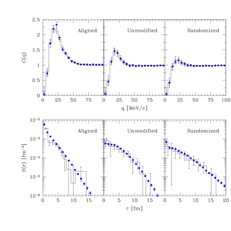
FIG. 1.: Upper panels: Original (solid symbols) and restored (histogram) proton correlation functions for different degrees of space-momentum alignment. The error bars in the original correlation functions are from the limited statistics of the RQMD runs. Lower panels: Reconstructed sources (histogram) and source computed directly in RQMD (solid symbols) for the different degrees of alignment.

Upper panels on Fig. 1 show the correlation functions for the three different cases. It is clear from the Figure that the degree of space-momentum correlation has a strong influence on the correlation function: the peak height of the correlation function changes from about 1.45 for unmodified RQMD to about 2.2 for the aligned case and 1.2 for randomized case. We would like to stress again, in all cases the spatial part of the source e.g. “radius” or “volume,” remains unaltered as does the transverse momentum spectrum and rapidity distribution of protons. Hence, the upper panels of Fig. 1 illustrate the danger of ignoring space-momentum correlations when analyzing correlation data.
On lower panels in Fig. 1 we show the proton sources obtained with the help of the imaging procedure outlined above. Notice that, as the degree of alignment increases (going from right to left), that the source function becomes narrower and higher.

FIG. 2.: Sketch of single particle sources at central rapidity, looking in the beam direction for the aligned case (left) and random case (right). The small circles represent the protons and the arrows represent their transverse momentum vectors. The areas outlined with the dashed lines represent regions where we find pairs with small relative momentum.

One can understand this shift to lower separations in the way sketched in Fig. 2. In the aligned case, it is more probable that nearby protons have a small relative momentum $q$. In the random case, any pair can have a small $q$, regardless of their separation. Given that the kernel cuts off contributions from pairs with larger $q$, we expect that the aligned case will have a narrower source than the unmodified case and the unmodified case will have a narrower source than the random case. Also, in Fig. 1 we have shown the sources constructed directly from the RQMD freeze-out distribution following eq. (5). In these sources, we considered all pairs with a relative momentum smaller than $q_{\rm cut}=60$ MeV/c. We explored a range of $q_{\rm cut}$ of 60 to 100 MeV/c, all beyond the point in the correlation where it is consistent with one, and found no cutoff dependence.
In all cases we see a general agreement of the imaged sources with the low relative momentum sources constructed directly from RQMD. In order to check the quality of the imaging and numerical stability of the inversion procedure, the two-proton correlation functions were calculated using the extracted relative source functions shown on lower panels in Fig. 1 as an input for eq. (1). The result of such “double inversion” procedure is shown on upper panels in Fig. 1 with solid circles. The agreement between the measured and reconstructed correlation function is quite good, confirming that imaging produces numerically stable and unbiased results.
In conclusion, we have explored the applicability of proton imaging to realistic sources with transverse space-momentum correlations. By fixing freeze-out spatial distribution and varying the degree of transverse space-momentum correlation we found that both the images and the two-particle correlation functions are very sensitive to these correlations. In particular, we have shown that the source function narrows (i.e. the probability of emitting pairs with small relative separation grows) and the peak of the proton correlation function increases as the degree of alignment increases. Finally, we have demonstrated that one can reliably reconstruct the source functions even with extreme transverse space-momentum correlations. We would like to point out that the effects of space-momentum correlations should be even more pronounced in the shapes of three-dimensional proton sources. Note that three dimensional proton imaging is now possible [27].
An important direction for the future is a detailed study of the change of the phase-space density and entropy (extracted from imaged sources [15]) with the varying degree of space-momentum correlation. Such work should provide information complementary to ongoing studies in the pion sector [28].
We gratefully acknowledge stimulating discussions with Drs. G. Bertsch, P. Danielewicz, D. Keane, A. Parreño, S Pratt, S. Voloshin and N. Xu. We also wish to thank Drs. R. Lednicky and J. Pluta for making their correlation afterburner code available. Finally, we thank Dr. H. Sorge for providing the code of the RQMD model. This research is supported by the U.S. Department of Energy grants DOE-ER-40561 and DE-FG02-89ER40531.

REFERENCES

- [1] S.E. Koonin, Phys. Lett. B70, 43 (1977).
- [2] T. Nakai and H. Yokomi, Prog. Theor. Phys. 66, 1328 (1981).
- [3] R. Lednicky and V.L. Lyuboshitz, Sov. J. Nucl. Phys. 35, 770 (1982).
- [4] D.J. Ernst, M.R. Strayer and A.S. Umar, Phys. Rev Lett. B55, 584 (1985).
- [5] W.G. Gong, W. Bauer, C.K. Gelbke, and S. Pratt, Phys. Rev. C43, 781 (1991).
- [6] S. Pratt, Nucl. Phys. A638, 125c (1998).
- [7] U.A Wiedemann and U. Heinz, Phys. Rep. 294, 1-165 (1998).
- [8] U. Heinz and B. Jacak, Ann. Rev. Nucl. Part. Sci 44, (1999).
- [9] T.C. Awes et al., WA80 Collaboration, Z.Phys. C65, 207 (1995).
- [10] S. Fritz et al., Aladin Collaboration, nucl-ex/9704002.
- [11] C. Schwartz et al., Aladin Collaboration, proc: 27th International Workshop on the Gross Properties of Nuclei and Nuclear Exitations, Hirschegg, 1999
- [12] S. Fritz et al., Aladin Collaboration, Phys. Lett. B315 (1999).
- [13] H. Appelshauser et al., NA49 Collaboration, nucl-ex/9905001, to appear Phys. Lett. B.
- [14] J. Barrette et al., E814/E877 Collaboration, Phys. Rev. C60: 054905 (1999).
- [15] D. A. Brown and P. Danielewicz. Phys. Lett. B398, 252 (1997).
- [16] D. A. Brown and P. Danielewicz. Phys. Rev. C57(5), 2474 (1998).
- [17] D.A. Brown, Accessing the Space-Time Development of Heavy-Ion Collisions With Theory and Experiment. PhD thesis, Michigan State University, 1998.
- [18] P. Danielewicz and D.A. Brown, nucl-th/9811048.
- [19] S.Y. Panitkin, E895 Collaboration, Proceedings of the 15th Winter Workshop on Nuclear Dynamics, Park City, Utah, January 1999
- [20] S. Pratt, Phys. Rev. Lett. 53, 1219 (1984).
- [21] S. Pratt, T. Csörgő, and J. Zimányi. Phys. Rev. C 42(6), 2646 (1990).
- [22] V. G. J. Stoks et al. Phys. Rev. C49, 2950 (1994).
- [23] P. Danielewicz and P. Schuck. Phys. Lett. B274, 268 (1992).
- [24] H. Sorge, Phys. Rev. C52, 3291 (1995).
- [25] M. Gmitro, J. Kvasil, R. Lednicky, V.L. Lyuboshitz, Czech. J. Phys. B36 (1986) 1281-1287.
- [26] B. Monreal et al., Phys. Rev. C60: 031901 (1999).
- [27] D.A. Brown, nucl-th/9904063.
- [28] D. Ferenc et al., Phys. Lett. B457, 347-352 (1999).