Mean-field nuclear structure calculations on a Basis-Spline Galerkin lattice

Abstract

Our goal is to carry out high-precision nuclear structure calculations in connection with Radioactive Ion Beam Facilities. The main challenge for the theory of drip line nuclei is that the outermost nucleons are weakly bound (implying a large spatial distribution) and that these states are strongly coupled to the particle continuum. For these reasons, the traditional basis expansion methods fail to converge. We overcome these problems by representing the nuclear Hamiltonian on a lattice utilizing the Galerkin method with Basis-Spline test functions. We discuss tests of the numerical method and applications to the deformed shell model, HF+BCS and HFB mean field theories.

1 Introduction

In recent years, the area of nuclear structure physics has shown substantial progress and rapid growth [1, 2]. With detectors such as GAMMASPHERE and EUROGAM, the limits of total angular momentum and deformation in atomic nuclei have been explored, and new neutron rich nuclei have been identified in spontaneous fission studies. Gamma-ray detectors under development such as GRETA [3] will have improved resolving power and should allow for the identification of weakly populated states never seen before in nuclei. Particularly exciting is the proposed construction of a next-generation ISOL FACILITY in the United States which has been been identified in the 1996 DOE/NSAC Long Range Plan [1] as the highest priority for major new construction.

These experimental developments as well as recent advances in computational physics have sparked renewed interest in nuclear structure theory. In contrast to the well-understood behavior near the valley of stability, there are many open questions as we move towards the proton and neutron driplines and towards the limits in mass number (superheavy region). While the proton dripline has been explored experimentally up to Z=83, the neutron dripline represents mostly “terra incognita”. In these exotic regions of the nuclear chart, one expects to see several new phenomena: near the neutron dripline, the neutron-matter distribution will be very diffuse and of large size giving rise to “neutron halos” and “neutrons skins”. One also expects new collective modes associated with this neutron skin, e.g. the “scissors” vibrational mode or the “pygmy” resonance. In proton-rich nuclei, we have recently seen both spherical and deformed proton emitters; this “proton radioactivity” is caused by the tunneling of weakly bound protons through the Coulomb barrier. The investigation of the properties of exotic nuclei is also essential for our understanding of nucleosynthesis in stars and stellar explosions (rp- and r-process). Our primary goal is to carry out high-precision nuclear structure calculations in connection with Radioactive Ion Beam Facilities. Some of the topics of interest are the effective N-N interaction at large isospin, large pairing correlations and their density dependence, neutron halos/skins, and proton radioactivity. Specifically, we are interested in calculating observables such as the total binding energy, charge radii, densities $\rho_{p,n}({\bf r})$, separation energies for neutrons and protons, pairing gaps, and potential energy surfaces.

There are many theoretical approaches to nuclear structure physics. For lack of space, we mention only three of these: in the macroscopic - microscopic method, one combines the liquid drop / droplet model with a microscopic shell correction from a deformed single-particle shell model (Möller and Nix [4], Nazarewicz et al. [5]). For relatively light nuclei, it is possible to diagonalize the nuclear Hamiltonian in a shell model basis. Barrett et al. [6] have recently carried out large-basis no-core shell model calculations for p-shell nuclei. A different approach to the interacting nuclear shell model is the Shell Model Monte Carlo (SMMC) method developed by Dean et al. [7] which does not involve matrix diagonalization but a path integral over auxiliary fields. This method has been applied to fp-shell and medium-heavy nuclei. Finally, for heavier nuclei one utilizes either nonrelativistic [8, 9, 10] or relativistic [11, 12] mean field theories.

2 Outline of the theory: HFB formalism in coordinate space

As we move away from the valley of stability, surprisingly little is known about the pairing force: For example, what is its density dependence? Large pairing correlations are expected near the drip lines which are no longer a small residual interaction. Neutron-rich nuclei are expected to be highly superfluid due to continuum excitation of neutron “Cooper pairs”. The Hartree-Fock-Bogoliubov (HFB) theory unifies the HF mean field theory and the BCS pairing theory into a single selfconsistent variational theory. The main challenge in the theory of exotic nuclei near the proton or neutron drip line is that the outermost nucleons are weakly bound (which implies a very large spatial extent), and that the weakly-bound states are strongly coupled to the particle continuum. This represents a major problem for mean field theories that are based on the traditional shell model basis expansion method in which one utilizes bound harmonic oscillator basis wavefunctions. As illustrated in Figure 1 a weakly bound state can still be reasonably well represented in the oscillator basis, but this is no longer true for the continuum states. In fact, Nazarewicz et al. [5] have shown that near the driplines the harmonic oscillator basis expansion does not converge even if $N=50$ oscillator quanta are used. This implies that one either has to use a continuum-shell model basis or one has to solve the problem directly on a coordinate space lattice. We have chosen the latter method.

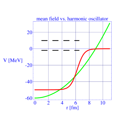
Figure 1: Inadequacy of shell model basis near the drip lines; need for high-accuracy lattice representation.

Several years ago, Umar et al. [13] have developed a three-dimensional HF code in Cartesian coordinates using the Basis-Spline discretization technique. The program is based on a density dependent effective N-N interaction (Skyrme force) which also includes the spin-orbit interaction. The code has proven efficient and extremely accurate; it incorporates BCS and Lipkin-Nogami pairing, and various constraints. The configuration space Hartree-Fock approach has had great successes in predicting systematic trends in the global properties of nuclei, in particular the mass, radii, and deformations across large regions of the periodic table.

So far, our attempts to generalize this 3D code to include self-consistent pairing forces (Hartree-Fock-Bogoliubov theory on the lattice) have proven too ambitious. The reason may be the lack of a suitable damping operator in 3D. We have therefore taken a different approach and developed a new Hartree-Fock + BCS pairing code in cylindrical coordinates for axially symmetric nuclei, based on the Galerkin method with B-Spline test functions [14, 15]. The new code has been written in Fortran 90 and makes extensive use of new data concepts, dynamic memory allocation and pointer variables. Extending this code, we believe that it will be easier to implement HFB in 2D because one can use highly efficient LAPACK routines to diagonalize the lattice Hamiltonian and does not necessarily rely on a damping operator.

We outline now our basic theoretical approach for lattice HFB. As is customary, we start by expanding the nucleon field operator into a complete orthonormal set of s.p. basis states $\phi_{i}$

$$\hat{\psi}^{\dagger}({\bf r},s)=\sum_{i}\ \hat{c}_{i}^{\dagger}\ \phi_{i}^{*}({\bf r},s)$$ (1)

which leads to the Hamiltonian in occupation number representation

$$\hat{H}=\sum_{i,j}<i|\ t\ |j>\ \hat{c}_{i}^{\dagger}\ \hat{c}_{j}\ +\frac{1}{4}\sum_{i,j,m,n}<ij|\ \tilde{v}^{(2)}\ |mn>\ \hat{c}_{i}^{\dagger}\ \hat{c}_{j}^{\dagger}\ \hat{c}_{n}\ \hat{c}_{m}\ .$$ (2)

Like in the BCS theory, one performs a canonical transformation to quasiparticle operators $\hat{\beta},\hat{\beta}^{\dagger}$

$$\left(\begin{array}[]{c}\hat{\beta}\\ \hat{\beta}^{\dagger}\end{array}\right)=\left(\begin{array}[]{cc}U^{\dagger}&V^{\dagger}\\ V^{T}&U^{T}\end{array}\right)\left(\begin{array}[]{c}\hat{c}\\ \hat{c}^{\dagger}\end{array}\right)\ .$$ (3)

The HFB ground state is defined as the quasiparticle vacuum

$$\hat{\beta}_{k}\ |\Phi_{0}>\ =\ 0\ .$$ (4)

The basic building blocks of the theory are the normal density

$$\rho_{ij}=<\Phi_{0}|\hat{c}_{j}^{\dagger}\ \hat{c}_{i}|\Phi_{0}>=(V^{*}V^{T})_{ij}$$ (5)

and the pairing tensor

$$\kappa_{ij}=<\Phi_{0}|\hat{c}_{j}\ \hat{c}_{i}|\Phi_{0}>=(V^{*}U^{T})_{ij}$$ (6)

from which one can form the generalized density matrix

$$\mathcal{R}=\left(\begin{array}[]{cc}\rho&\kappa\\ -\kappa^{*}&1-\rho^{*}\end{array}\right)\ \Rightarrow\mathcal{R}^{\dagger}=\mathcal{R},\ \mathcal{R}^{2}=\mathcal{R}\ .$$ (7)

Using the definition of the HFB ground state energy

$$E^{\prime}(\mathcal{R})=<\Phi_{0}|\hat{H}-\lambda\hat{N}|\Phi_{0}>$$ (8)

we derive the equations of motion from the variational principle

$$\delta\ [E^{\prime}(\mathcal{R})-{\rm{tr}}\ \Lambda(\mathcal{R}^{2}-\mathcal{R})]\ =\ 0$$ (9)

which results in the standard HFB equations

$$[\mathcal{H},{\mathcal{R}}]\ =\ 0$$ (10)

with the generalized single-particle Hamiltonian

$$\mathcal{H}=\left(\begin{array}[]{cc}h&\Delta\\ -\Delta^{*}&-h^{*}\end{array}\right);\ h=\partial E^{\prime}/\partial\rho,\ \Delta=\partial E^{\prime}/\partial\kappa^{*}\ .$$ (11)

Our goal is to transform to a coordinate space representation and solve the resulting differential equations on a lattice. For this purpose, we define two types of quasi-particle wavefunctions $\phi_{1},\phi_{2}$

$$\phi_{1}^{*}(E_{n},{\bf r}\sigma)\ =\ \sum_{i}U_{in}\ \phi_{i}({\bf r}\sigma)\ ,\ \ \ \phi_{2}(E_{n},{\bf r}\sigma)\ =\ \sum_{i}V_{in}^{*}\ \phi_{i}({\bf r}\sigma)$$ (12)

in terms of which the particle density matrix for the HFB ground state assumes a very simple mathematical structure [9]

$$\rho_{0}\ ({\bf r},\sigma,{\bf r}^{\prime},\sigma^{\prime})\ =\ <\Phi_{0}|\ \hat{\psi}^{\dagger}({\bf r}^{\prime}\sigma^{\prime})\ \hat{\psi}({\bf r}\sigma)\ |\Phi_{0}>$$

$$=\sum_{i,j}\rho_{ij}\ \phi_{i}({\bf r}\sigma)\ \phi_{j}^{*}({\bf r}^{\prime}\sigma^{\prime})=\sum_{E_{n}>0}^{\infty}\phi_{2}(E_{n},{\bf r}\sigma)\ \phi_{2}^{*}(E_{n},{\bf r}^{\prime}\sigma^{\prime})\ .$$ (13)

In a similar fashion we obtain for the pairing tensor

$$\kappa_{0}\ ({\bf r},\sigma,{\bf r}^{\prime},\sigma^{\prime})\ =\ <\Phi_{0}|\ \hat{\psi}({\bf r}^{\prime}\sigma^{\prime})\ \hat{\psi}({\bf r}\sigma)\ |\Phi_{0}>$$

$$=\sum_{i,j}\kappa_{ij}\ \phi_{i}({\bf r}\sigma)\ \phi_{j}({\bf r}^{\prime}\sigma^{\prime})=\sum_{E_{n}>0}^{\infty}\phi_{2}(E_{n},{\bf r}\sigma)\ \phi_{1}^{*}(E_{n},{\bf r}^{\prime}\sigma^{\prime})\ .$$ (14)

For certain types of effective interactions (e.g. Skyrme forces) the HFB equations in coordinate space are local and have a structure which is reminiscent of the Dirac equation [9]

$$\left(\matrix{(h-\lambda)&\tilde{h}\cr\tilde{h}&-(h-\lambda)\cr}\right)\left(\matrix{\phi_{1}({\bf r})\cr\phi_{2}({\bf r})\cr}\right)=E\left(\matrix{\phi_{1}({\bf r})\cr\phi_{2}({\bf r})\cr}\right)\ ,$$ (15)

where $h$ is the “particle” Hamiltonian and $\tilde{h}$ denotes the “pairing” Hamiltonian.

The various terms in $h$ depend on the particle densities $\rho_{q}(\bf r)$ for protons and neutrons, on the kinetic energy density $\tau_{q}(\bf r)$, and on the spin-current tensor $J_{ij}(\bf r)$. The pairing Hamiltonian $\tilde{h}$ has a similar structure, but depends on the pairing densities $\tilde{\rho}_{q}(\bf r),\tilde{\tau}_{q}(\bf r)$ and $\tilde{J}_{ij}(\bf r)$ instead. Because of the structural similarity between the Dirac equation and the HFB equation in coordinate space, we encounter here similar computational challenges: for example, the spectrum of quasiparticle energies $E$ is unbounded from above and below. The spectrum is discrete for $|E|<-\lambda$ and continuous for $|E|>-\lambda$. In the case of axially symmetric nuclei, the spinor wavefunctions $\phi_{1}({\bf r})$ and $\phi_{2}({\bf r})$ have the structure

$$\psi^{\Omega}(\phi,r,z)=\frac{1}{\sqrt{2\pi}}\left(\matrix{e^{i(\Omega-\frac{1}{2})\phi}\ U(r,z)\cr e^{i(\Omega+\frac{1}{2})\phi}\ L(r,z)\cr}\right)\ .$$ (16)

3 Computational method: Spline-Galerkin lattice representation

For nuclei near the p/n driplines, we overcome the convergence problems of the traditional shell-model expansion method by representing the nuclear Hamiltonian on a lattice utilizing a Basis-Spline expansion [16, 15, 14]. B-Splines $B_{i}^{M}(x)$ are piecewise-continuous polynomial functions of order $(M-1)$. They represent generalizations of finite elements which are B-splines with $M=2$. A set of fifth-order B-Splines is shown in Figure 2.

Figure 2: Set of fifth-order B-Splines for fixed boundary conditions.

Let us now discuss the Galerkin method with B-Spline test functions. We consider an arbitrary (differential) operator equation

$${\cal{O}}\bar{f}(x)-\bar{g}(x)=0\;.$$ (17)

Special cases include eigenvalue equations of the HF/HFB type where ${\cal{O}}=h$ and $\bar{g}(x)=E\bar{f}(x)$. We assume that both $\bar{f}(x)$ and $\bar{g}(x)$ are well approximated by Spline functions

$$\bar{f}(x)\approx f(x)\equiv\sum_{i=1}^{\cal N}B_{i}^{M}(x)a^{i}\;,\ \ \ \ \bar{g}(x)\approx g(x)\equiv\sum_{i=1}^{\cal N}B_{i}^{M}(x)b^{i}\;.$$ (18)

Because the functions $f(x)$ and $g(x)$ are approximations to the exact functions $\bar{f}(x)$ and $\bar{g}(x)$, the operator equation will in general only be approximately fulfilled

$${\cal{O}}f(x)-g(x)=R(x)\;.$$ (19)

The quantity $R(x)$ is called the residual; it is a measure of the accuracy of the lattice representation. We multiply the last equation from the left with the spline function $B_{k}(x)$ and integrate over $x$

$$\int v(x)dxB_{k}(x){\cal{O}}f(x)-\int v(x)dxB_{k}(x)g(x)=\int v(x)dxB_{k}(x)R(x)\;\;.$$ (20)

We have included a volume element weight function $v(x)$ in the integrals to emphasize that the formalism applies to arbitrary curvilinear coordinates. Various schemes exist to minimize the residual function $R(x)$; in the Galerkin method one requires that there be no overlap between the residual and an arbitrary B-spline function

$$\int v(x)dxB_{k}(x)R(x)=0\;\;.$$ (21)

This so called Galerkin condition amounts to a global reduction of the residual. Applying the Galerkin condition and inserting the B-Spline expansions for $f(x)$ and $g(x)$ results in

$$\sum_{i}\left[\int v(x)dxB_{k}(x){\cal{O}}B_{i}(x)\right]a^{i}-\sum_{i}\left[\int v(x)dxB_{k}(x)B_{i}(x)\right]b^{i}=0\;\;.$$ (22)

Defining the matrix elements

$${\cal{O}}_{ki}=\int v(x)dxB_{k}(x){\cal{O}}B_{i}(x)\;\;,\ \ G_{ki}=\int v(x)dxB_{k}(x)B_{i}(x)\;$$ (23)

transforms the (differential) operator equation into a matrix $\times$ vector equation

$$\sum_{i}{\cal{O}}_{ki}a^{i}=\sum_{i}G_{ki}b^{i}\;$$ (24)

which can be implemented on modern vector or parallel computers with high efficiency. The matrix $G_{ki}$ is sometimes referred to as the Gram matrix; it represents the nonvanishing overlap integrals between different B-Spline functions (see Fig. 2). We eliminate the expansion coefficients $a^{i},\ b^{i}$ in the last equation by introducing the function values at the lattice support points $x_{\alpha}$ including both interior and boundary points.

The upper $(U)$ and lower $(L)$ components of the spinor wavefunctions defined earlier are represented on the 2-D lattice $(r_{\alpha},z_{\beta})$ by a product of Basis Splines $B_{i}(x)$ evaluated at the lattice support points

$$U(r_{\alpha},z_{\beta})=\sum_{i,j}B_{i}(r_{\alpha})\ B_{j}(z_{\beta})\ U^{ij}\ ,\ \ \ L(r_{\alpha},z_{\beta})=\sum_{i,j}B_{i}(r_{\alpha})\ B_{j}(z_{\beta})\ L^{ij}\ .$$ (25)

We are also extending our previous B-spline work to include nonlinear grids. Use of a nonlinear lattice should be most useful for loosely bound systems near the proton or neutron drip lines. Non-Cartesian coordinates necessitate the use of fixed endpoint boundary conditions; much effort has been directed toward improving the treatment of these boundaries [14].

4 Numerical tests and results

We expect our Spline techniques to be superior to the traditional harmonic oscillator basis expansion method in cases of very strong nuclear deformation. To illustrate this point, we have performed a numerical test using a phenomenological (Woods-Saxon) deformed shell model potential. We calculate the single-particle energy spectrum for neutrons in ${}^{40}Ca$ for quadrupole deformations ranging from strong oblate ($\beta_{2}=-1.25$) to extreme prolate ($\beta_{2}=+2.25$). The results are shown in Fig. 3. Apparently, for $\beta_{2}=0$ we correctly reproduce the spherical shell structure of magic nuclei. As $\beta_{2}$ approaches large positive values our s.p. potential approaches the structure of two separated potential wells; as expected, we observe pairs of levels with opposite parity that are becoming degenerate in energy. The largest quadrupole deformation corresponds physically to a symmetric fission configuration. Clearly, such configurations cannot be described in a single oscillator basis, which confirms the numerical superiority of the B-Spline lattice technique.

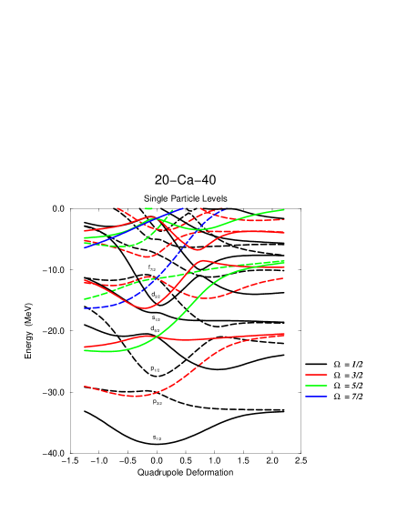
Figure 3: Single-particle neutron levels for ${}^{40}_{20}Ca$ as function of quadrupole deformation in the Woods-Saxon shell model. Solid lines indicate positive parity and broken lines negative parity levels.

In a second test calculation, we have investigated the properties of a nucleus near the neutron drip line. During the last decade the discovery of a ‘neutron halo’ in several neutron-rich isotopes generated a great deal of interest in the area of weakly bound quantum systems. The halo effect was first observed in ${}^{11}_{\ 3}$Li, which consists of three protons and six neutrons in a central core and two planetary neutrons which comprise the halo. By adjusting the depth of the Woods-Saxon potential so that the separation energy of the last bound neutron is only $10$ keV, i.e. very close to the continuum, we were able to determine this neutron wavefunction on the lattice which shows a very large spatial extent (see Fig. 4). We conclude that the B-Spline lattice techniques are well-suited for representing weakly bound states near the drip lines; a similar calculation in the basis expansion method would require a large number of oscillator shells.

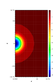
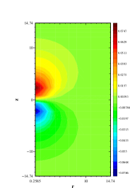
Figure 4: (a) Woods Saxon potential for ${}^{11}_{\ 3}$Li; (b) spin-up component of the wave function for the last bound neutron.

We now discuss our numerical results for the selfconsistent Hartree-Fock calculations with Skyrme-M^∗ interaction and BCS pairing. This is a special case of the HFB equation with a constant pairing matrix element. In Fig. 5 we display the proton density for a heavy nucleus, ${}^{154}_{\ 64}$Gd, calculated with our new 2-D (HF+BCS) code. It should be noted that ALL 154 nucleons are treated dynamically (no inert core approximation). The theoretical charge density looks quite similar to the experimental result which is shown on the right hand side.

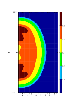
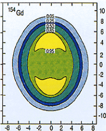
Figure 5: Proton density for ${}^{154}_{\ 64}$Gd, (a) calculated with the 2-D Skyrme Hartree-Fock + BCS pairing code; (b) measured charge distribution.

For several spherical nuclei, we have also compared the selfconsistent s.p. energy levels of our 2-D Spline-Galerkin code with a fully converged 1-D radial calculation. The result is shown in Table 1.

Table 1: Total binding energy and s.p. energy levels for ${}^{16}O$, calculated in the Hartree-Fock + BCS pairing theory with the SkM^∗ force. Comparison of results from 1D radial finite difference code [17] and our new 2D Spline-Galerkin code. We obtain the same level of accuracy despite the $25$ times larger lattice spacing $\Delta=0.625$ fm.

	1D Radial	2D Spline-Galerkin
	$\Delta=0.025$fm	$\Delta=0.625$fm
$E_{tot}$	-127.73 MeV	-127.48 MeV
$E_{s1/2}(n)$	-33.31 MeV	-33.29 MeV
$E_{p3/2}(n)$	-19.88 MeV	-19.86 MeV
$E_{p1/2}(n)$	-13.55 MeV	-13.53 MeV
$E_{s1/2}(p)$	-29.74 MeV	-29.72 MeV
$E_{p3/2}(p)$	-16.48 MeV	-16.45 MeV
$E_{p1/2}(p)$	-10.27 MeV	-10.26 MeV

4.1 Plans and Future Directions

Having validated our new (HF+BCS) code on a 2D lattice with the Spline-Galerkin method, we plan to proceed as follows: We are currently working on the 2D HFB implementation with a pairing delta-force. After that, we will generalize the code utilizing the full SkP force with mean pairing field and pairing spin-orbit term. We will also add appropriate constraints, e.g. $Q_{20},Q_{30},\omega j_{x}$ for calculating potential energy surfaces and rotational bands. As we compare the observables (e.g. total binding energy, charge radii, densities $\rho_{p,n}({\bf r})$, separation energies for neutrons and protons, pairing gaps) with experimental data from the RIB facilities, it will almost certainly be necessary to develop new effective N-N interactions as we move farther away from the stability line towards the p/n drip lines.

References

- [1] “Nuclear Science: A Long Range Plan”, DOE/NSF Nuclear Science Advisory Committee (Feb. 1996)
- [2] “Scientific Opportunities with an Advanced ISOL Facility”, Panel Report (Nov. 1997), ORNL
- [3] I.Y. Lee et al., Int. Conf. NUCLEAR STRUCTURE ’98, Gatlinburg, TN (Aug. 1998), Abstracts p.76
- [4] P. Möller, J.R. Nix and K.L. Kratz, Atomic Data Nucl. Data Tables 66, 131 (1997)
- [5] W. Nazarewicz, T.R. Werner and J. Dobaczewski, Phys. Rev. C 50, 2860 (1994)
- [6] P. Navratil, B.R. Barrett and W.E. Ormand, Phys. Rev. C 56, 2542, (1997)
- [7] S.E. Koonin, D.J. Dean, and K. Langanke, Phys. Rep. 278, 1 (1997)
- [8] J. Dobaczewski, H. Flocard, and J. Treiner, Nucl. Phys. A422 (1984) 103.
- [9] J. Dobaczewski, W. Nazarewicz, T.R. Werner, J.F. Berger, C.R. Chinn, and J. Dechargé, Phys. Rev. C53 (1996) 2809.
- [10] P.-G. Reinhard, M. Bender, K. Rutz, and J. A. Maruhn, Z. Phys. A358 (1997) 277.
- [11] W. Nazarewicz, J. Dobaczewski, T.R. Werner, J.A. Maruhn, P.-G. Reinhard, K.Rutz, C.R. Chinn, A.S. Umar, M.R. Strayer, Phys. Rev. C53, 740 (1996).
- [12] W. Pöschl, D. Vretenar, G.A. Lalazissis and P. Ring, Phys. Rev. Lett. 79, 3841 (1997)
- [13] C.R. Chinn, A.S. Umar, M. Vallieres, and M.R. Strayer, Phys. Rev. E50, 5096 (1994).
- [14] D.R. Kegley, V.E. Oberacker, M.R. Strayer, A.S. Umar, and J.C. Wells, J. Comp. Phys. 128 (1996) 197.
- [15] D.R. Kegley, Ph.D. thesis, Vanderbilt University (1996)
- [16] J.C. Wells, V.E. Oberacker, M.R. Strayer and A.S. Umar, Int. J. Mod. Phys. C6 (1995) 143
- [17] P.-G. Reinhard, Univ. Erlangen, PGRAD Fortran-77 code.