The Two-Nucleon Sector with Effective Field Theory

I present the results obtained for several observables in the two-nucleon sector using effective field theory with KSW power-counting and dimensional regularization. In addition to the phase shifts for nucleon-nucleon scattering, several deuteron observables are discussed, including electromagnetic form factors, polarizabilities, $\gamma d\rightarrow\gamma d$ Compton scattering, and $np\rightarrow d\gamma$. A detailed comparison between the effective field theory with pions, the theory without pions, and effective range theory is made.

1 Introduction

During the last year there has been a tremendous effort to understand the role of effective field theory (EFT) in the two- and three-nucleon sectors$\!{}^{{\bf?}}$^-$\!{}^{{\bf?}}$. Since the previous Nuclear Physics with Effective Field Theory workshop held twelve months ago at Caltech I have been primarily focused on exploring the implications of KSW power counting$\!{}^{{\bf?}}$ in the two-nucleon sector. In addition to the nucleon-nucleon scattering phase shifts in the spin-singlet ${}^{1}\kern-1.4ptS_{0}$ and spin-triplet ${}^{3}\kern-1.4ptS_{1}$ channels, various properties of the deuteron and processes involving the deuteron have been considered.

If one is interested in the static properties of the deuteron or very low-energy ($|{\bf p}|\ll m_{\pi}$) nucleon-nucleon scattering the pion can be “integrated” out of the theory, leaving a very simple EFT involving only nucleons and external currents (we will denote this theory as ${\rm EFT}({\pi\hskip-6.00006pt/})$). The simplicity of the theory allows for many observables to be computed up to next-to-next-to-leading order (NNLO) with ease$\!{}^{{\bf?}}$, and enables a direct comparison with effective range theory$\!{}^{{\bf?},{\bf?}}$ to be made. The expansion parameter in ${\rm EFT}({\pi\hskip-6.00006pt/})$ is $Q\sim|{\bf p}|/m_{\pi}$, which for static properties of the deuteron corresponds to $Q\sim{1\over 3}$. A direct comparison between ${\rm EFT}({\pi\hskip-6.00006pt/})$ and effective range theory shows that effective range theory reproduces EFT up to the order at which multi-nucleon-external-current operators enter. At that order and beyond, effective range theory fails to reproduce effective field theory, and thus is an incomplete description of the strong interactions.

For processes involving higher momenta, such as $|{\bf p}|\raisebox{-3.01385pt}{$\stackrel{{\scriptstyle\textstyle>}}{{\sim}}$ }m_{\pi}$, the pions must be included as a dynamical field. In KSW power-counting, the exchange of potential pions is a subleading interaction compared to the momentum-independent, quark mass independent four-nucleon operator, and is treated in perturbation theory. Some have questioned the convergence of perturbative pions$\!{}^{{\bf?}}$, and we will see that for the deuteron observables we have considered the subleading contribution from potential pion exchange is smaller than the contribution from higher derivative four-nucleon operators. While this does not directly answer the questions raised by Cohen and Hansen $\!{}^{{\bf?}}$, it is an important observation. For the static properties of the deuteron, one recovers the results of the ${\rm EFT}({\pi\hskip-6.00006pt/})$ with corrections suppressed by terms higher order in ${\rm EFT}({\pi\hskip-6.00006pt/})$, as expected.

2 EFFECTIVE FIELD THEORY WITH PIONS

2.1 THE NUCLEON-NUCLEON INTERACTION

The two-nucleon sector contains length scales that are much larger than one would naively expect from QCD. Scattering lengths in the s-wave channels are $a^{({}^{1}\kern-0.98ptS_{0})}=-23.7\ {\rm fm}$ in the ${}^{1}\kern-1.4ptS_{0}$ channel and $a^{({}^{3}\kern-0.98ptS_{1})}=5.4\ {\rm fm}$ in the ${}^{3}\kern-1.4ptS_{1}$ channel, much greater than both $1/\Lambda_{\chi}\sim 0.2\ {\rm fm}$ and $1/f_{\pi}\sim 1.5\ {\rm fm}$, typical hadronic scales.

Figure 1: The phase shift $\delta^{({}^{1}\kern-0.98ptS_{0})}$ verses the momentum of each nucleon in the center-of-mass. The solid line denotes the Nijmegen partial wave analysis of the experimental data.

The solid curve in fig. (1) shows the phase shift in the ${}^{1}\kern-1.4ptS_{0}$ channel, $\delta^{({}^{1}\kern-0.98ptS_{0})}$, from the Nijmegen partial wave analysis$\!{}^{{\bf?}}$ of the experimental data. $\delta^{({}^{1}\kern-0.98ptS_{0})}$ rises very fast at low momentum and then turns over at about $|{\bf p}|\sim 40\ {\rm MeV}$.

The lagrange density that describes the interaction between two S-wave nucleons has the form

$${\cal L} = -C_{0}^{({}^{1}\kern-0.98ptS_{0})}(N^{T}P^{a}N)^{\dagger}(N^{T}P^{a}N)-D_{2}^{({}^{1}\kern-0.98ptS_{0})}\omega\ Tr[m_{q}](N^{T}P^{a}N)^{\dagger}(N^{T}P^{a}N)$$ (1)

$$+{C_{2}^{({}^{1}\kern-0.98ptS_{0})}\over 8}\left[(N^{T}P^{a}N)^{\dagger}\left(N^{T}P^{a}(\overrightarrow{\bf\nabla}-\overleftarrow{\bf\nabla})^{2}N\right)+h.c.\right]$$

$$-g_{A}N^{\dagger}{\bf\sigma}\cdot{\bf A}N\ +\ ({}^{3}\kern-1.4ptS_{1})\ +\ ...$$

where the ellipses denote terms with more insertions of the small expansion parameters $Q\sim m_{q}$ and $Q\sim\nabla$. The reason for writing such an expansion is that one hopes or expects that QCD will give rise to S-matrix elements for multiple nucleon processes that have a systematic expansion in the light quark masses and in external momenta. Only interactions in the ${}^{1}\kern-1.4ptS_{0}$ channel are explicitly shown in Eq. (1), while interactions in the ${}^{3}\kern-1.4ptS_{1}$ channel are denoted by “$({}^{3}\kern-1.4ptS_{1})$”. In addition, terms from $D_{2}$ involving pion field operators (required by chiral symmetry), and terms involving the photon field are not explicitly shown in Eq. (1). ${\bf A}$ is the axial vector meson field. The $P^{a}$ is a spin-isospin projector, $P^{a}={1\over\sqrt{8}}\sigma_{2}\tau_{2}\tau^{a}$, projects onto the ${}^{1}\kern-1.4ptS_{0}$ channel.

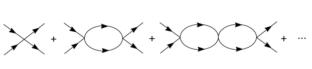
Figure 2: The leading contribution to nucleon-nucleon scattering arising from local operators.

NN scattering in the ${}^{1}\kern-1.4ptS_{0}$ channel receives contributions at leading order from the graphs shown in fig. (2), i.e the bubble-chain of contact operators. Choosing the coefficient $C_{0}^{({}^{1}\kern-0.98ptS_{0})}$ to reproduce the scattering length gives the dot-dashed curve in fig (1). At subleading order, there are contributions from the $C_{2},D_{2}$ operators, in addition to the exchange of a potential pion, as shown in fig (3). The best fit to the phase shift for momenta less than $\sim 250~{}{\rm MeV}$ is shown by the dashed curve in fig (1), while the fit that reproduces both the scattering length and effective range is shown as the dotted curve in fig (1).

Figure 3: Graphs contributing to the subleading amplitude ${\cal A}_{0}$. The shaded ovals correspond to the bubble chain in Fig. (2) and free propagation.

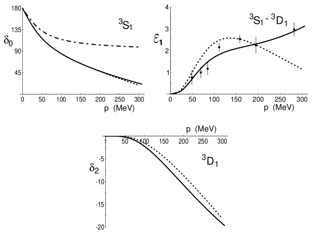
Figure 4: The phase shifts $\delta_{0}$, $\delta_{2}$ and mixing parameter $\overline{\varepsilon}_{1}$ for the ${}^{3}\kern-1.4ptS_{1}-{}^{3}\kern-1.4ptD_{1}$ channel. The solid line denotes the results of the Nijmegen partial wave analysis. The dot-dashed curve is the fit at order $Q^{-1}$ for $\delta_{0}$, while $\delta_{2}=\overline{\varepsilon}_{1}=0$ at this order. The dashed curves are the results of the order $Q^{0}$ fit of $\delta_{0}$ to the partial wave analysis over the momentum range $p\leq 200\ {\rm\ MeV}$.

Analysis of scattering in the ${}^{3}\kern-1.4ptS_{1}-{}^{3}\kern-1.4ptD_{1}$ channel is a straightforward extension of the analysis in the ${}^{1}\kern-1.4ptS_{0}$ channel. The important difference is that the nucleons in the initial and final states with total angular momentum $J=1$ can be in an orbital angular momentum state of either $L=0$ or $L=2$. The S-matrix describing scattering in the coupled channel $J=1$ system is written as

$$S = \left(\matrix{e^{i2\delta_{0}}\cos 2\overline{\varepsilon}_{1}&ie^{i(\delta_{0}+\delta_{2})}\sin 2\overline{\varepsilon}_{1}\cr ie^{i(\delta_{0}+\delta_{2})}\sin 2\overline{\varepsilon}_{1}&e^{i2\delta_{2}}\cos 2\overline{\varepsilon}_{1}}\right)\ \ \ ,$$ (2)

where we use the “barred” parameterization of $\!{}^{{\bf?}}$, also used in $\!{}^{{\bf?}}$. The power counting for amplitudes that take the nucleons from a ${}^{3}\kern-1.4ptS_{1}$-state to a ${}^{3}\kern-1.4ptS_{1}$-state is identical to the analysis in the ${}^{1}\kern-1.4ptS_{0}$-channel. Operators between two ${}^{3}\kern-1.4ptD_{1}$ states are not directly renormalized by the leading operators, which project out only ${}^{3}\kern-1.4ptS_{1}$ states. However, they are renormalized by operators that mix the ${}^{3}\kern-1.4ptS_{1}$ and ${}^{3}\kern-1.4ptD_{1}$ states, which in turn are renormalized by the leading interactions. Further, they involve a total of four spatial derivatives, two on the incoming nucleons, and two on the out-going nucleons. Therefore, such operators contribute at order $Q^{3}$, and can be neglected in the present computation. Consequently, amplitudes for scattering from an ${}^{3}\kern-1.4ptD_{1}$ state into an ${}^{3}\kern-1.4ptD_{1}$ state are dominated by single potential pion exchange at order $Q^{0}$. Operators connecting ${}^{3}\kern-1.4ptD_{1}$ and ${}^{3}\kern-1.4ptS_{1}$ states are renormalized by the leading operators, but only on the $L=0$ “side” of the operator. Therefore the coefficient of this operator, $C_{2}^{(sd)}\sim Q^{-1}$, indicates that this interaction contributes at order $Q^{1}$ and can be neglected at order $Q^{0}$. Thus, mixing between ${}^{3}\kern-1.4ptD_{1}$ and ${}^{3}\kern-1.4ptS_{1}$ states is dominated by single potential pion exchange dressed by a bubble chain of $C_{0}^{({}^{3}\kern-0.98ptS_{1})}$ operators. A parameter free prediction for this mixing exists at order $Q^{0}$. The dashed curves in Fig. (4) show the phase shifts $\delta_{0}$, $\delta_{2}$ and mixing parameter $\overline{\varepsilon}_{1}$ compared to the Nijmegen partial wave analysis$\!{}^{{\bf?}}$ for this set of coefficients. There are no free parameters at this order in either $\overline{\varepsilon}_{1}$ or $\delta_{2}$.

2.2 THE DEUTERON

Electromagnetic Form Factors and Moments

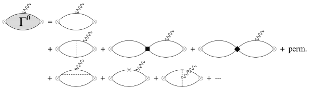
Figure 5: The diagrams contributing to the electric form factors of the deuteron.

Once the Lagrange density in the nucleon sector has been established the standard tools of field theory can be used to determine the properties of the deuteron$\!{}^{{\bf?}}$. To compute the electromagnetic form factors of the deuteron one first computes the three point correlation function between a source that creates a nucleon pair in a ${}^{3}\kern-1.4ptS_{1}$ state, a source that destroys a nucleon pair in a ${}^{3}\kern-1.4ptS_{1}$ state and a source that creates a photon. After LSZ reduction and wavefunction renormalization one obtains the electromagnetic form factors. Leading order (LO), next-to-leading (NLO) and next-to-next-to-leading order (NNLO) graphs contributing to the electric form factors of the deuteron are shown in Fig. (5).

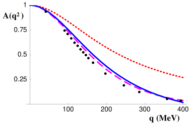
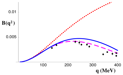
Figure 6: The form factors $A(q^{2})$ and $B(q^{2})$ measured in elastic electron-deuteron scattering. The dotted curve is the LO prediction, while the solid curve NLO prediction. The dashed curve is the prediction of effective range theory. There is one counterterm contributing to $B(q^{2})$ at this order which is fixed by the deuteron magnetic moment.

The resulting form factors $A(q^{2})$ and $B(q^{2})$ that appear in the differential cross section for electron deuteron scattering are shown in Fig. (6). $A(q^{2})$ is dominated by the charge form factor and $B(q^{2})$ depends only upon the magnetic form factor. One sees that the form factors computed at subleading order agree well with the data. The charge radius of the deuteron is found to be

$$\sqrt{<r^{2}>}_{\rm th} = {1\over 2\sqrt{2}\gamma}\ +\ C_{2}(\mu){M_{N}(\mu-\gamma)^{2}\over 8\sqrt{2}\pi}\ +\ {g_{A}^{2}M_{N}m_{\pi}^{2}(3m_{\pi}+10\gamma)\over 48\sqrt{2}\pi f_{\pi}^{2}(m_{\pi}+2\gamma)^{3}}\ +\ ...$$

$$= 1.53\ \ +\ \ 0.36\ \ +\ \ ...\ \ =\ \ 1.89\ {\rm fm}+...$$

$$\sqrt{<r^{2}>}_{\rm expt} = 2.11\ {\rm fm}\ \ \ ,$$ (3)

where $\gamma=\sqrt{M_{N}B}$ is the binding momentum of the deuteron. In computing the numerical value we have used the numerical value of $C_{2}$ extracted from a fit to data over the range of momenta $|{\bf p}|<250\ {\rm MeV}$. Given the expansion parameter for the theory is $\sim{1\over 3}$, we expect $\sqrt{<r^{2}>}_{\rm th}$ given in Eq. (3) is within $\sim 10\%$ of the actual value, which it is.

In effective range theory the electromagnetic form factors are assumed to be dominated by the asymptotic S-wave deuteron wave function,

$$\psi^{({\rm ER})}({\bf r}) = \sqrt{{\gamma\over 2\pi(1-\gamma r_{0})}}{e^{-\gamma r}\over r}\ \ \ .$$ (4)

Assuming the small r part of the deuteron wave function is only important for establishing the normalization condition, $F_{C}(0)=1$, the prediction of effective range theory for the form factor $F_{C}(q^{2})$ follows from the Fourier transform of $|\psi^{(ER)}({\bf r})|^{2}$,

$$F^{(ER)}_{C}(q^{2})=\left({1\over 1-\gamma\rho_{d}}\right)\left(\left({4\gamma\over\sqrt{-q^{2}}}\right){\rm tan}^{-1}\left({\sqrt{-q^{2}}\over 4\gamma}\right)-\gamma\rho_{d}\right)\ \ \ .$$ (5)

This yields a deuteron charge radius,

$$\sqrt{\langle r_{d}^{2}\rangle^{\rm ER}} = {1\over 2\sqrt{2}\gamma}{1\over\sqrt{1-\gamma\rho_{d}}}$$ (6)

$$= {1\over 2\sqrt{2}\gamma}\left[1+{1\over 2}\gamma\rho_{d}\ +{3\over 8}\gamma^{2}\rho_{d}^{2}\ +\ ...\right]\ \ \ ,$$

which gives a numerical value of $\sqrt{\langle r_{d}^{2}\rangle^{\rm ER}}=1.98~{}{\rm fm}$, very close to the quoted value of the matter radius of the deuteron$\!{}^{{\bf?},{\bf?}}$ of $r_{m}=1.967\pm 0.002~{}{\rm fm}$. Conventionally, the charge radius is obtained by combining the nucleon charge radius in quadrature with the matter radius, which agrees very well with the experimental value.

Expanding the EFT expression for $\sqrt{<r^{2}>}_{\rm th}$ in Eq. (3) in powers of $\gamma/m_{\pi}$, we have

$$\gamma\ll m_{\pi} \rightarrow {1\over 2\sqrt{2}\gamma}\left[1+{1\over 2}\gamma r_{0}\ +\ {g_{A}^{2}M_{N}\gamma\over 4\pi f_{\pi}^{2}}{\gamma^{2}\over m_{\pi}^{2}}\ +\ ...\right]\ \ \ ,$$ (7)

where $r_{0}$ is the effective range. It is clear that the NLO calculation is the same order as a single insertion of $r_{0}$, but there is also a contribution arising from pion exchange that is beyond effective range theory.

The quadrupole moment vanishes at leading order in the expansion but receives a contribution at subleading order from the exchange of one potential pion, giving

$$\mu_{{\cal Q},th} = {g_{A}^{2}M_{N}(6\gamma^{2}+9m_{\pi}\gamma+4m_{\pi}^{2})\over 30\pi f_{\pi}^{2}(m_{\pi}+2\gamma)^{3}}\ +\ ....$$

$$= 0.40\ {\rm fm^{2}}\ +...$$

$$\mu_{{\cal Q},expt} = 0.2859\ {\rm fm^{2}}\ \ \ ,$$ (8)

which is approximately $30\%$ larger than the experimental value. Clearly, a NNLO calculation$\!{}^{{\bf?}}$ is needed to ensure that the EFT value is indeed converging to the experimental value.

In contrast, there is a local counterterm contributing to the magnetic moment at NLO,

$$\mu_{M} = \mu_{p}\ +\ \mu_{n}\ +\ L_{2}(\mu){\gamma\over 2\pi}(\mu-\gamma)^{2}\ +\ ...$$ (9)

$$= 0.88\ -\ 0.02\ \ \ (fit)\ \ \ \ ,$$

which determines the counterterm $L_{2}$ at the scale $\mu$. Once this counterterm has been determined from the deuteron magnetic moment, the entire form factor $B(q^{2})$ is determined to NLO.

Polarizabilities

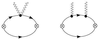
Figure 7: The leading diagrams contributing to the electric polarizability of the deuteron. Crossed graphs are not shown.

The scalar $\alpha_{E0}$ and tensor $\alpha_{E2}$ electric polarizabilities are found to be$\!{}^{{\bf?}}$

$$\alpha_{E0} = {\alpha M_{N}\over 32\gamma^{4}}\ +\ {\alpha M_{N}^{2}\over 64\pi\gamma^{3}}C_{2}(\mu)(\mu-\gamma)^{2}$$

$$+ {\alpha g_{A}^{2}M_{N}^{2}\over 384\pi f^{2}}\ {m_{\pi}^{2}(3m_{\pi}^{2}+16m_{\pi}\gamma+24\gamma^{2})\over\gamma^{3}(m_{\pi}+2\gamma)^{4}}\ +\ ...$$

$$\alpha_{E2} = -{\alpha g_{A}^{2}M_{N}^{2}\over 80\pi f^{2}}\ {2m_{\pi}^{3}+11m_{\pi}^{2}\gamma+16m_{\pi}\gamma^{2}+8\gamma^{3}\over\gamma^{2}(m_{\pi}+2\gamma)^{4}}$$

$$\alpha_{E0} = 0.595\ {\rm fm}^{3}\ +\ ...\ \ ,\ \ \alpha_{E2}=-0.062\ {\rm fm}^{3}\ +\ ...\ \ \ .$$ (10)

Numerically, the value of $\alpha_{E0}$ in Eq. (10) is expected to be within $\sim 10\%$ of the actual value. Potential models, which find a value of$\!{}^{{\bf?}}$ $\alpha_{E0}=0.632\pm 0.003\ {\rm fm}^{3}$, are expected to reproduce this observable to high precision as the short-distance contributions are expected to be small.

It is informative to perform a momentum expansion of $\alpha_{E0}$ to make contact with effective range theory,

$$\alpha_{E0} \rightarrow {\alpha M_{N}\over 32\gamma^{4}}\left[1\ +\ C_{2}(\mu)\ {M_{N}\gamma(\mu-\gamma)^{2}\over 2\pi}\right.$$ (11)

$$\left.\qquad\qquad\ +\ {g_{A}^{2}M_{N}\gamma\over 4\pi f^{2}}\left(1-{8\over 3}{\gamma\over m_{\pi}}+{16\over 3}{\gamma^{2}\over m_{\pi}^{2}}\ +\ ...\right)\right]$$

$$= {\alpha M_{N}\over 32\gamma^{4}}\left[1\ +\ \gamma r_{0}\ +\ {g_{A}^{2}M_{N}\gamma\over 4\pi f^{2}}{10\over 3}{\gamma^{2}\over m_{\pi}^{2}}\ +\ ...\right]\ \ \ .$$

The momentum expansion of Eq. (10) agrees with effective range theory up to order $\gamma^{2}$ at linear order in $r_{0}$. The deviations from effective range theory arise from the electromagnetic interactions of the pions, which are beyond effective range theory.

$\gamma$-Deuteron Compton Scattering

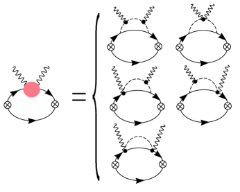
Figure 8: Pion graphs that contribute to the nucleon polarizabilities and to $\gamma$-deuteron Compton scattering at NLO. The crossed circles denote operators that create or annihilate two nucleons with the quantum numbers of the deuteron. The dark solid circles correspond to the photon coupling via the nucleon or pion kinetic energy operator or via the gauged axial pion-nucleon interaction. The solid lines are nucleons and the dashed lines are pions. The photon crossed graphs are not shown.

A process that may allow for a determination of the neutron polarizabilities (given the proton polarizabilities) is $\gamma$-deuteron Compton scattering. In power counting the graphs that contribute to the deuteron polarizability, it was assumed$\!{}^{{\bf?}}$ that $E_{\gamma}\sim|{\bf p}_{\gamma}|\sim Q^{2}$. However, for Compton scattering at photon energies of $\sim 100\ {\rm MeV}$, the appropriate scaling is $E_{\gamma}\sim|{\bf p}_{\gamma}|\sim Q$. With this power counting (called Regime II counting$\!{}^{{\bf?}}$), the nucleon isoscalar polarizabilities contribute at NLO through the graphs shown in fig (8).

The cross section for $\gamma$-deuteron Compton scattering$\!{}^{{\bf?}}$ up to NLO is shown in fig (9) for incident photon energies of $E_{\gamma}~{}=~{}49~{}{\rm MeV}$ and $69~{}{\rm MeV}$.

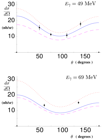
Figure 9: The differential cross section for $\gamma$-deuteron Compton scattering at incident photon energies of $E_{\gamma}=49\ {\rm MeV}$ and $69\ {\rm MeV}$. The dashed curves correspond to the LO result. The dotted curves correspond to the NLO result without the graphs that contribute to the polarizability of the nucleon. The solid curves correspond to the complete NLO result with no free parameters, as described in the text. Systematic and statistical errors associated with each data point have been added in quadrature.

There are no published data for this cross section, but there is unpublished data in the PhD Thesis of M. Lucas$\!{}^{{\bf?}}$, consisting of four data points at $E_{\gamma}=49\ {\rm MeV}$ and two data points at $E_{\gamma}=69\ {\rm MeV}$. In fig (9) the dashed curve is the LO calculation which is consistently below the data. The dotted curve is the NLO calculation with the nucleon polarizabilities resulting from the graphs in fig (8) set equal to zero. This overestimates the cross section, with the exception of the back angle data point at $E_{\gamma}=49\ {\rm MeV}$. The solid curve is the complete NLO calculation which agrees reasonably well with the data.

There are two published potential model calculations of this cross section$\!{}^{{\bf?},{\bf?}}$. Their results disagree with each other at the $\sim 10-15\%$ level, and do not reproduce the data at both energies. A more sophisticated potential model calculation has recently been completed by Karakowski and Miller$\!{}^{{\bf?}}$. Further, a calculation of this process is being performed using Weinberg’s power counting by Beane, Philips and van Kolck$\!{}^{{\bf?}}$. In the near future more data is expected to become available which will allow for a clearer picture of our understanding of this process.

$np\rightarrow d\gamma$

One of the classic nuclear physics processes is the radiative capture $np\rightarrow d\gamma$. It is a clear demonstration of the existence of “meson exchange currents” in nuclei. The cross section for this process has been measured long ago, and for neutrons incident in the lab with speed $|{\bf v}|=2200\ {\rm m/s}$, the cross section is $\sigma^{\rm expt}=334.2\pm 0.5\ {\rm mb}$$\!{}^{{\bf?}}$. The theoretical cross section for this process has been calculated with effective range theory$\!{}^{{\bf?},{\bf?}}$, and also more recently using a potential model motivated by Weinberg’s power counting$\!{}^{{\bf?}}$.

The amplitude for the radiative capture of extremely low momentum neutrons $np\rightarrow d\gamma$ has contributions from both the ${}^{1}\kern-1.4ptS_{0}$ and ${}^{3}\kern-1.4ptS_{1}$ $NN$ channels. It can be written as

$$i{\cal A} = e\ X\ N^{T}\tau_{2}\ \sigma_{2}\ \left[{\bf\sigma}\cdot{\bf k}\ \ {\bf\epsilon}(d)^{*}\cdot{\bf\epsilon}(\gamma)^{*}\ -\ {\bf\sigma}\cdot{\bf\epsilon}(\gamma)^{*}\ \ {\bf k}\cdot{\bf\epsilon}(d)^{*}\right]N$$

$$+ ie\ Y\ \epsilon^{ijk}\ \epsilon(d)^{i*}\ k^{j}\ {\bf\epsilon}(\gamma)^{k*}\ (N^{T}\tau_{2}\tau_{3}\sigma_{2}N)\ \ \ \ ,$$

where $e=|e|$ is the magnitude of the electron charge, $N$ is the doublet of nucleon spinors, ${\bf\epsilon}(\gamma)$ is the polarization vector for the photon, ${\bf\epsilon}(d)$ is the polarization vector for the deuteron and ${\bf k}$ is the outgoing photon momentum. The term with coefficient $X$ corresponds to capture from the ${}^{3}\kern-1.4ptS_{1}$ channel while the term with coefficient $Y$ corresponds to capture from the ${}^{1}\kern-1.4ptS_{0}$ channel. For convenience, we define dimensionless variables $\tilde{X}$ and $\tilde{Y}$, by

$$X = i{2\over M_{N}}\sqrt{\pi\over\gamma^{3}}\ \tilde{X}\ \ ,\ \ Y=i{2\over M_{N}}\sqrt{\pi\over\gamma^{3}}\ \tilde{Y}\ \ \ \ .$$ (13)

Both $\tilde{X}$ and $\tilde{Y}$ have the $Q$ expansions, $\tilde{X}=\tilde{X}_{0}+\tilde{X}_{1}+...$, and $\tilde{Y}=\tilde{Y}_{0}+\tilde{Y}_{1}+...$, where a subscript $n$ denotes a contribution of order $Q^{n}$.

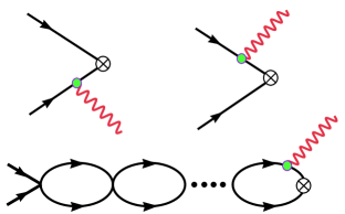
Figure 10: Graphs contributing to the amplitude for $np\rightarrow d\gamma$ at leading order in the effective field theory expansion. The solid lines denote nucleons and the wavy lines denote photons. The light solid circles correspond to the nucleon magnetic moment coupling to the electromagnetic field. The crossed circle represents an insertion of the deuteron interpolating field which is taken to have ${}^{3}\kern-1.4ptS_{1}$ quantum numbers.

At leading order in the EFT$\!{}^{{\bf?}}$ the graphs shown in fig (10) give a contribution to the cross section of

$$\sigma^{LO}={8\pi\alpha\gamma^{5}\kappa_{1}^{2}(a^{({}^{1}\kern-0.98ptS_{0})})^{2}\over|{\bf v}|M_{N}^{5}}\left(1-{1\over\gamma a^{({}^{1}\kern-0.98ptS_{0})}}\right)^{2}\ =\ 297.2\ {\rm mb}\ \ \ .$$ (14)

This agrees with the effective range theory calculation of Bethe and Longmire $\!{}^{{\bf?}}$ and Noyes $\!{}^{{\bf?}}$ when terms in their expression involving the effective range are neglected. Eq. (14) is about $10\%$ less than the experimental value, $\sigma^{\rm expt}=334.2\pm 0.5\ {\rm mb}$$\!{}^{{\bf?}}$.

At NLO there are contributions from insertions of the $C_{2},D_{2}$ operators and from potential pion exchange with the isovector nucleon magnetic moment.

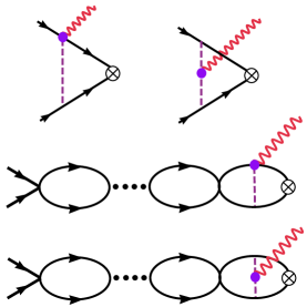
Figure 11: Pion exchange current contributions to the amplitude for $np\rightarrow d\gamma$ arising at NLO. The solid lines denote nucleons and the wavy lines denote photons. The dashed line denotes a pion. The dark solid circles correspond to minimal coupling of the photon. The crossed circle represents an insertion of the deuteron interpolating field.

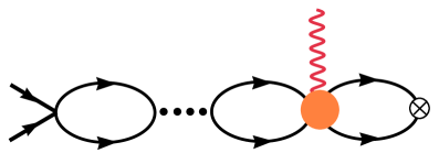
Figure 12: Local counterterm contribution to the amplitude for $np\rightarrow d\gamma$ at NLO. The solid lines denote nucleons and the wavy lines denote photons. The solid circle corresponds to an insertion of the $L_{1}$ operator. The crossed circle represents an insertion of the deuteron interpolating field. The graphs corresponding to final state interactions are not shown.

In addition, there are contributions from meson exchange where the photon is minimally coupled either to the axial current or to the pion itself. These diagrams, shown in fig (11), are called “meson exchange currents”. Also, at this order there is a contribution from a four-nucleon-one-photon counterterm, shown in fig (12). The contributions from the meson exchange currents and the counterterm$\!{}^{{\bf?}}$ are

$$\tilde{Y}^{(\rm\pi,E)} = {g_{A}^{2}M_{N}\gamma^{2}\over 12\pi f^{2}}\left({m_{\pi}-\gamma\over(m_{\pi}+\gamma)^{2}}\right.$$

$$\left.\qquad\qquad\ +\ {M_{N}\over 4\pi}{\cal A}_{-1}^{({}^{1}\kern-0.98ptS_{0})}(0)\left({3m_{\pi}-\gamma\over 2(m_{\pi}+\gamma)}+{\rm ln}\left({m_{\pi}+\gamma\over\mu}\right)-{1\over 6}+\delta\right)\right)$$

$$\tilde{Y}^{(\rm L_{1})} = L_{1}\ \gamma^{2}\ {{\cal A}_{-1}^{({}^{1}\kern-0.98ptS_{0})}(0)\over\bar{C}_{0}^{({}^{1}\kern-0.98ptS_{0})}\bar{C}_{0}^{({}^{3}\kern-0.98ptS_{1})}}\ \ \ ,$$ (15)

where $\delta$ is a subtraction constant. The important point to note here is that the contribution from the meson exchange currents is UV divergent, as is clear from the presense of the $\log(\mu)$ contribution in eq. (15), and the subtraction constant $\delta$. This divergence is absorbed by the local counterterm $L_{1}(\mu)$, and therefore it makes no sense to discuss the contribution from meson exchange currents alone.

The two four-nucleon-one-photon counterterms that arise at NLO are renormalized very differently. In contrast to the counterterm $L_{1}(\mu)$, the counterterm $L_{2}(\mu)$ is not driven by meson exchange currents and satisfies a simple renormalization group equation,

$$\mu{d\over d\mu}\left[{L_{1}-{1\over 2}\kappa_{1}\left(C_{2}^{({}^{1}\kern-0.98ptS_{0})}+C_{2}^{({}^{3}\kern-0.98ptS_{1})}\right)\over\bar{C}_{0}^{({}^{1}\kern-0.98ptS_{0})}\bar{C}_{0}^{({}^{3}\kern-0.98ptS_{1})}}\right] = {g_{A}^{2}M^{2}\over 48\pi^{2}f^{2}}$$

$$\mu{d\over d\mu}\left[{L_{2}\over(\bar{C}_{0}^{({}^{3}\kern-0.98ptS_{1})})^{2}}\right] = 0\ \ \ .$$ (16)

3 EFFECTIVE FIELD THEORY WITHOUT PIONS

For processes involving external momenta much less than the pion mass, it is much simpler to work with an EFT where the pions do not appear. In this pionless theory$\!{}^{{\bf?}}$ (${\rm EFT}({\pi\hskip-6.00006pt/})$), one can examine each of the observables we have just discussed in the theory with dynamical pions. In many of the cases the calculation can be pushed to higher order with little effort, which makes the pionless theory particularly attractive for static properties. Without pions the only expansion parameter is the external momentum, $Q\sim{\bf p}$, where we will neglect the electromagnetic interaction and isospin breaking$\!{}^{{\bf?}}$.

3.1 THE NUCLEON-NUCLEON INTERACTION

In ${\rm EFT}({\pi\hskip-6.00006pt/})$, the mixing parameter $\overline{\varepsilon}_{1}$ is supressed by $Q^{2}$ compared with $\delta_{0}^{(0)}$, and therefore, up to N⁴LO, we can isolate the S-wave from the D-wave in the deuteron channel, leaving

$$S_{00} = e^{i2\delta_{0}}\ =\ 1\ +\ {2i\over\cot\delta_{0}-i}\ \ \ \ .$$ (17)

The phase shift $\delta_{0}$ has an expansion in powers of $Q$, $\delta_{0}=\delta_{0}^{(0)}+\delta_{0}^{(1)}+\delta_{0}^{(2)}+~{}...$, where the superscript denotes the order in the $Q$ expansion. By forming the logarithm of both sides of eq. (17) and expanding in powers of $Q$, it is straightforward to obtain

$$\delta_{0}^{(0)}(|{\bf k}|) = \pi-\tan^{-1}\left({|{\bf k}|\over\gamma}\right)$$

$$\delta_{0}^{(1)}(|{\bf k}|) = -{\rho_{d}\over 2}|{\bf k}|$$

$$\delta_{0}^{(2)}(|{\bf k}|) = -\left[{\rho_{d}^{2}\gamma\over 4}+{\gamma^{3}\over 8M_{N}^{2}(\gamma^{2}+|{\bf k}|^{2})}\right]|{\bf k}|\ \ \ ,$$ (18)

which are shown in fig. (13).

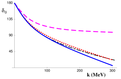
Figure 13: The phase shift in the ${}^{3}\kern-1.4ptS_{1}$ channel, $\delta_{0}$, as a function of the center of mass momentum $|{\bf k}|$. The dashed curve corresponds to $\delta_{0}^{(0)}$, the dotted curve corresponds to $\delta_{0}^{(0)}+\delta_{0}^{(1)}$, the solid curve corresponds to $\delta_{0}^{(0)}+\delta_{0}^{(1)}+\delta_{0}^{(2)}$, and the dot-dashed curve is the Nijmegen partial wave analysis$\!{}^{{\bf?}}$.

Up to NNLO, the shape parameter term, $w_{2}$ does not contribute to the S-wave phase shift and therefore, in addition to being numerically small (about a factor of 5 smaller than $\rho_{d}$), $w_{2}$ enters only at higher orders. Formally, the first deviations from linear $|{\bf k}|$ dependence at large momenta arises from relativistic corrections (the second term in $\delta_{0}^{(2)}$ in eq. (18). The $Q$ expansion is clearly demonstrated in eq. (18), by simply counting powers of $|{\bf k}|$ and $\gamma$, which both scale like $Q$. We expect this perturbative expansion of the phase shifts to converge up to momenta of order $\sim m_{\pi}/2\sim 70~{}{\rm MeV}$, at which point one encounters the t-channel cut from potential pion exchange.

Scattering between the S-wave and D-wave is induced by local operators first arising at $Q^{1}$ in the power counting. At order $Q^{1}$ and $Q^{2}$, the lagrange density describing such interaction is

$${\cal L}^{(sd)}_{2} = {1\over 4}{{}^{\pi\hskip-2.625pt/}\hskip-1.99997ptC_{0}^{(sd)}}\left(N^{T}P^{i}N\right)^{\dagger}\left(N^{T}{\cal O}^{(sd),xyj}N\right){\cal T}^{ijxy}\ +\ {\rm h.c.}$$ (19)

$$- {1\over 16}{{}^{\pi\hskip-2.625pt/}\hskip-1.99997ptC_{2}^{(sd)}}\left(N^{T}\left[P_{i}\overrightarrow{\bf D}^{2}+\overleftarrow{\bf D}^{2}P_{i}-2\overleftarrow{\bf D}P_{i}\overrightarrow{\bf D}\right]N\right)^{\dagger}\left(N^{T}{\cal O}^{(sd),xyj}N\right){\cal T}^{ijxy}\ +\ {\rm h.c.}\ \ \ ,$$

where

$${\cal O}^{(sd),xyj} = \overleftarrow{\bf D}^{x}\overleftarrow{\bf D}^{y}P^{j}+P^{j}\overrightarrow{\bf D}^{x}\overrightarrow{\bf D}^{y}-\overleftarrow{\bf D}^{x}P^{j}\overrightarrow{\bf D}^{y}-\overleftarrow{\bf D}^{y}P^{j}\overrightarrow{\bf D}^{x}$$

$${\cal T}^{ijxy} = \left(\delta^{ix}\delta^{jy}-{1\over n-1}\delta^{ij}\delta^{xy}\right)\ \ \ ,$$ (20)

and where $n$ is the number of spacetime dimensions. The lagrange density in eq. (20) appears somewhat complex. However, when the electromagnetic field is ignored, the operator collapses to

$${\cal O}^{(sd),xyj} \rightarrow P^{j}\left(\overleftarrow{\bf\nabla}-\overrightarrow{\bf\nabla}\right)^{x}\left(\overleftarrow{\bf\nabla}-\overrightarrow{\bf\nabla}\right)^{y}\ \ \ ,$$ (21)

explicitly Galilean invariant.

The coefficients that appear in eq. (20) themselves have an expansion in powers of $Q$, e.g. ${{}^{\pi\hskip-2.625pt/}\hskip-1.99997ptC_{0}^{(sd)}}={{}^{\pi\hskip-2.625pt/}\hskip-1.99997ptC_{0,-1}^{(sd)}}+{{}^{\pi\hskip-2.625pt/}\hskip-1.99997ptC_{0,0}^{(sd)}}+...$. Performing a $Q$ expansion on the mixing parameter $\overline{\varepsilon}_{1}=\overline{\varepsilon}^{(2)}_{1}+\overline{\varepsilon}^{(3)}_{1}+...$ it is straightforward to demonstrate that

$$\overline{\varepsilon}_{1}^{(2)}(|{\bf k}|) = {\sqrt{2}\over 3}\left({{{}^{\pi\hskip-2.625pt/}\hskip-1.99997ptC_{0,-1}^{(sd)}}\over{{}^{\pi\hskip-2.625pt/}\hskip-1.99997ptC_{0,-1}^{({}^{3}\kern-0.98ptS_{1})}}}\right){|{\bf k}|^{3}\over\sqrt{\gamma^{2}+|{\bf k}|^{2}}}$$ (22)

$$= -{M_{N}\over 4\pi}(\mu-\gamma){\sqrt{2}\over 3}\ {{}^{\pi\hskip-2.625pt/}\hskip-1.99997ptC_{0,-1}^{(sd)}}{|{\bf k}|^{3}\over\sqrt{\gamma^{2}+|{\bf k}|^{2}}}\ \ \ .$$

Renormalization group invariance of this leading order contribution to $\overline{\varepsilon}_{1}$ indicates that ${{}^{\pi\hskip-2.625pt/}\hskip-1.99997ptC_{0,-1}^{(sd)}}\propto(\mu-\gamma)^{-1}$. Renormalizing at the scale $\mu=m_{\pi}$, and fitting to the Nijmegen phase shift analysis$\!{}^{{\bf?}}$, we find ${{}^{\pi\hskip-2.625pt/}\hskip-1.99997ptC_{0,-1}^{(sd)}}=-4.57\ {\rm fm}^{4}$.

At the next order, $Q^{3}$, the contribution to $\overline{\varepsilon}_{1}$ is

$$\overline{\varepsilon}_{1}^{(3)}(|{\bf k}|) = -{\sqrt{2}\over 3}{M_{N}\over 4\pi}\left[\left({\mu\gamma\rho_{d}\over 2}\ {{}^{\pi\hskip-2.625pt/}\hskip-1.99997ptC_{0,-1}^{(sd)}}\ +\ (\mu-\gamma)\ {{}^{\pi\hskip-2.625pt/}\hskip-1.99997ptC_{0,0}^{(sd)}}\right){|{\bf k}|^{3}\over\sqrt{\gamma^{2}+|{\bf k}|^{2}}}\right.$$ (23)

$$\left.\qquad\ +\ \left({\rho_{d}\over 2}\ {{}^{\pi\hskip-2.625pt/}\hskip-1.99997ptC_{0,-1}^{(sd)}}+(\mu-\gamma)\ {{}^{\pi\hskip-2.625pt/}\hskip-1.99997ptC_{2,-2}^{(sd)}}\ \right){|{\bf k}|^{5}\over\sqrt{\gamma^{2}+|{\bf k}|^{2}}}\right]\ \ \ ,$$

where we have expanded ${{}^{\pi\hskip-2.625pt/}\hskip-1.99997ptC_{2}^{(sd)}}={{}^{\pi\hskip-2.625pt/}\hskip-1.99997ptC_{2,-2}^{(sd)}}+...$. The first term in eq. (23) has the same momentum dependence as, $\overline{\varepsilon}_{1}^{(2)}$ the leading contribution in eq. (22). In the same way that we have required the position of the deuteron pole is not modified by higher orders in perturbation theory, we may require that the coefficient contributing to $\overline{\varepsilon}_{1}^{(2)}$ is not modified by higher order contributions. This constraint leads to

$${{}^{\pi\hskip-2.625pt/}\hskip-1.99997ptC_{0,0}^{(sd)}} = -{\mu\gamma\rho_{d}\over 2(\mu-\gamma)}\ {{}^{\pi\hskip-2.625pt/}\hskip-1.99997ptC_{0,-1}^{(sd)}}\ \ \ .$$ (24)

Further, as the second term in eq. (23) is an observable, we obtain the RG equation

$$\mu{d\over d\mu}\left({\rho_{d}\over 2}\ {{}^{\pi\hskip-2.625pt/}\hskip-1.99997ptC_{0,-1}^{(sd)}}+(\mu-\gamma)\ {{}^{\pi\hskip-2.625pt/}\hskip-1.99997ptC_{2,-2}^{(sd)}}\ \right) = 0\ \ \ ,$$ (25)

The only free parameter ${{}^{\pi\hskip-2.625pt/}\hskip-1.99997ptC_{2,-2}^{(sd)}}=+41.0~{}{\rm fm}^{6}$ (renormalized at $\mu=m_{\pi}$) is fit to the Nijmegen phase shift analysis$\!{}^{{\bf?}}$, as shown in fig. (14).

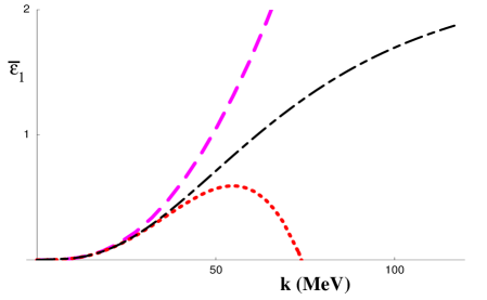
Figure 14: The S-D mixing parameter $\overline{\varepsilon}_{1}$ as a function of the center of mass momentum $|{\bf k}|$. The dashed curve corresponds to $\overline{\varepsilon}_{1}^{(2)}$, the dotted curve corresponds to $\overline{\varepsilon}_{1}^{(2)}+\overline{\varepsilon}_{1}^{(3)}$, and the dot-dashed curve is the Nijmegen partial wave analysis.

Electric Polarizability of the Deuteron

With the ${\rm EFT}({\pi\hskip-6.00006pt/})$ we have computed $\alpha_{E0}$ up to NNLO, including relativistic corrections. It has a perturbative expansion in $Q$, and we write $\alpha_{E0}=\alpha_{E0}^{(-4)}+\alpha_{E0}^{(-3)}+\alpha_{E0}^{(-2)}+...$. Explicit calculation gives

$$\alpha_{E0}^{(-4)}+\alpha_{E0}^{(-3)}+\alpha_{E0}^{(-2)} = {\alpha M_{N}\over 32\gamma^{4}}\left[1\ \ +\ \ \gamma\rho_{d}\ \ +\ \ \gamma^{2}\rho_{d}^{2}\ \ +\ \ {2\gamma^{2}\over 3M_{N}^{2}}\right]$$ (26)

$$= \qquad 0.377\ +\ 0.153\ +\ 0.062\ +\ 0.0006\$$

$$= 0.592~{}{\rm fm}^{3}\ \ \ .$$

Numerically, the relativistic corrections are very small, two orders of magnitude smaller than the NNLO corrections from the four-nucleon interactions. The value of $\alpha_{E0}$ in Eq. (26) is within $\sim 5\%$ of that computed with potential models and with effective range theory. Despite being numerically small, relativistic corrections can be calculated easily with the EFT. The S-wave-D-wave mixing operators (corresponding to the D-wave component of the deuteron in potential model language) make contributions to $\alpha_{E}^{(-2)}$. They do not contribute to the scalar polarizability, $\alpha_{E0}^{(-2)}$, but do contribute to the tensor polarizability, $\alpha_{E2}^{(-2)}$. Such operators will contribute to $\alpha_{E0}$ at higher orders in the expansion.

Electromagnetic Form Factors of the Deuteron

The charge radius of the deuteron at NNLO one finds in ${\rm EFT}({\pi\hskip-6.00006pt/})$ is

$$\langle r_{d}^{2}\rangle^{\rm EFT} = \langle r_{N,0}^{2}\rangle\ +\ {1\over 8\gamma^{2}}\left[1\ +\ \gamma\rho_{d}\ +\ \gamma^{2}\rho_{d}^{2}\right]\ +\ {1\over 32M_{N}^{2}}$$ (27)

$$= 0.62\ \ \ \ +\ \ \ \ 2.33\ +\ 0.95\ +\ 0.39\ +\ 0.0014$$

$$= 4.30~{}{\rm fm}^{2}\ \ \ \ ,$$

where the last term is the relativistic correction. Taking the square root of this value gives $\sqrt{\langle r_{d}^{2}\rangle}=2.07~{}{\rm fm}$, which is within a few percent of the measured value of $\sqrt{\langle r_{d}^{2}\rangle}=2.1303~{}{\rm fm}$$\!{}^{{\bf?},{\bf?},{\bf?},{\bf?}}$.

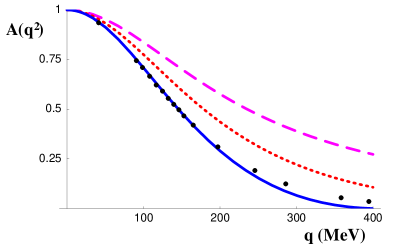
Figure 15: The form factor $A(q^{2})$ as a function of $|{\bf q}|=\sqrt{-q^{2}}$. The dashed curve corresponds to the LO prediction, the dotted curve corresponds to the NLO prediction, and the solid curve corresponds to the NNLO prediction, in ${\rm EFT}({\pi\hskip-6.00006pt/})$.

At NLO the deuteron magnetic moment is

$$\mu_{d} = {e\over 2M_{N}}\left(\kappa_{p}\ +\ \kappa_{n}\ +\ {{}^{\pi\hskip-2.625pt/}\hskip-1.99997ptL_{2}}\ {2M_{N}\gamma(\mu-\gamma)^{2}\over\pi}\right)\ \ \ ,$$ (28)

the same expression as is found in the theory with pions. Comparing the numerical value of this expression with the measured value of $\mu_{d}$ gives (at NLO)

$${{}^{\pi\hskip-2.625pt/}\hskip-1.99997ptL_{2}}(m_{\pi}) = -0.149\ {\rm fm^{4}}\ \ \ \ ,$$ (29)

at the renormalization scale $\mu=m_{\pi}$. The evolution of the ${{}^{\pi\hskip-2.625pt/}\hskip-1.99997ptL_{2}}(\mu)$ operator as the renormalization scale is changed is determined by the RG equation

$$\mu{d\over d\mu}\left[{{{}^{\pi\hskip-2.625pt/}\hskip-1.99997ptL_{2}}\over\left({{}^{\pi\hskip-2.625pt/}\hskip-1.99997ptC_{0,-1}^{({}^{3}\kern-0.98ptS_{1})}}\right)^{2}}\right] = 0\ \ \ \ .$$ (30)

It is combinations of the electric, magnetic and quadrupole form factors that are measured in elastic electron-deuteron scattering. The differential cross section for unpolarized elastic electron-deuteron scattering is given by

$${{\rm d}\sigma\over{\rm d}\Omega}={{\rm d}\sigma\over{\rm d}\Omega}\biggl{|}_{\rm Mott}\biggr{.}\left[A(q^{2})+B(q^{2})\tan^{2}\left({\theta\over 2}\right)\right]\ \ \ \ ,$$ (31)

where $A$ and $B$ are related to the form factors$\!{}^{{\bf?}}$ by

$$A = F_{C}^{2}+{2\over 3}\eta F_{M}^{2}+{8\over 9}\eta^{2}F_{\cal Q}^{2}\ \ \ \ ,$$

$$B = {4\over 3}\eta(1+\eta)F_{M}^{2}\ ,$$ (32)

with $\eta=-q^{2}/4M_{d}^{2}$. In order to compare with data, we take our analytic results for the form factors and expand the expression eq. (32) in powers of $Q$. At the order we are working, $A$ is sensitive both the electric and magnetic form factors, while $B$ depends only on the magnetic form factor. The predictions for $A(q^{2})$ and $B(q^{2})$ along with data are shown in fig. (15) and fig. (16), respectively.

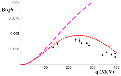
Figure 16: The form factor $B(q^{2})$ as a function of $|{\b{q}}|=\sqrt{-q^{2}}$. The dashed curve corresponds to the LO prediction, and the dotted curve corresponds to the NLO prediction, in ${\rm EFT}({\pi\hskip-6.00006pt/})$.

Numerically, one finds that the quadrupole moment is given by the sum of $\mu_{\cal Q}^{(0)}=0.273\ {\rm fm^{2}}$ and $\mu_{\cal Q}^{(1)}=\left(0.160\ -\ 0.0165\ {{}^{\pi\hskip-2.625pt/}\hskip-1.99997ptC_{\cal Q}}\right)\ {\rm fm^{2}}$ giving, at NLO,

$$\mu_{\cal Q} = \left(0.433\ -\ 0.0165\ {{}^{\pi\hskip-2.625pt/}\hskip-1.99997ptC_{\cal Q}}\right)\ {\rm fm^{2}}\ \ \ ,$$ (33)

where ${{}^{\pi\hskip-2.625pt/}\hskip-1.99997ptC_{\cal Q}}$ is the coefficient of a four-nucleon-one-photon operator, and is measured in ${\rm fm^{5}}$. Setting ${{}^{\pi\hskip-2.625pt/}\hskip-1.99997ptC_{\cal Q}}=0$, we find a quadrupole moment of $0.433\ {\rm fm^{2}}$, which is to be compared with the measured value of $0.287\ {\rm fm^{2}}$. In order to reproduce the measured value of the quadrupole moment ${{}^{\pi\hskip-2.625pt/}\hskip-1.99997ptC_{\cal Q}}=+8.9\ {\rm fm^{5}}$, at $\mu=m_{\pi}$. The quadrupole form factor resulting from this fit is shown in fig. (17).

Figure 17: The quadrupole form factor $F_{\cal Q}(|{\bf k}|^{2})$ as a function of $|{\bf k}|$. The dashed curve corresponds to the LO prediction, and the dotted curve corresponds to the NLO prediction, in ${\rm EFT}({\pi\hskip-6.00006pt/})$. The dot-dashed curve corresponds to a calculation with the Bonn-B potential in the formulation of $\!{}^{{\bf?}}$ .

$np\rightarrow d\gamma$

In ${\rm EFT}({\pi\hskip-6.00006pt/})$ we find a cross section for $np\rightarrow d\gamma$, at NLO and at $|{\bf v}|=2200~{}{\rm m/s}$ incident neutron speed, of

$$\sigma_{{\pi\hskip-2.625pt/}} = \left(287.1\ +\ 6.51\ {{}^{\pi\hskip-2.625pt/}\hskip-1.99997ptL_{1}}\ \right)\ {\rm mb}\ \ \ \ ,$$ (34)

where ${{}^{\pi\hskip-2.625pt/}\hskip-1.99997ptL_{1}}$ is the coefficient of a four-nucleon-one-magnetic-photon operator, with units of ${\rm fm}^{4}$ and is renormalized $\mu=m_{\pi}$. Requiring $\sigma_{{\pi\hskip-2.625pt/}}$ to reproduce the measured cross section $\sigma^{\rm expt}$ fixes ${{}^{\pi\hskip-2.625pt/}\hskip-1.99997ptL_{1}}=7.24~{}{\rm fm}^{4}$.

We see that even in the theory without dynamical pions, one is able to recover the cross section for radiative neutron capture at higher orders. It is clear that in this theory the four-nucleon-one-photon operators play a central role in reproducing the low energy observables. In the theory with pions, one can see by examining the contributing Feynman diagrams$\!{}^{{\bf?}}$, that in the limit that the momentum transferred to the photon is small the pion propagators can be replaced by $1/m_{\pi}^{2}$, while keeping the derivative structure in the numerator. This contribution, as well as the contribution from all hadronic exchanges, is reproduced order by order in the momentum expansion by the contributions from local multi-nucleon-photon interactions. From the calculations in the theory with dynamical pions, the value of ${{}^{\pi\hskip-2.625pt/}\hskip-1.99997ptL_{1}}$ is not saturated by pion exchange currents as these contributions are divergent, and require the presense of the $L_{1}$ operator$\!{}^{{\bf?}}$. Therefore, estimates of ${{}^{\pi\hskip-2.625pt/}\hskip-1.99997ptL_{1}}$ based on meson exchanges alone are model dependent.

The effective range calculation of $np\rightarrow d\gamma$ was first performed by Bethe and Longmire$\!{}^{{\bf?}}$ and revisited by Noyes$\!{}^{{\bf?}}$. After correcting the typographical errors in the expression for $\sigma$ that appears in the Noyes article, the expressions in the two papers$\!{}^{{\bf?},{\bf?}}$ are identical,

$$\sigma^{({\rm ER})} = {2\pi\alpha\ \kappa_{1}^{2}\ \gamma^{6}\ (a^{({}^{1}\kern-0.98ptS_{0})})^{2}\ a^{({}^{3}\kern-0.98ptS_{1})}\over|{\bf v}|M_{N}^{5}\left(2\ -\ \gamma a^{({}^{3}\kern-0.98ptS_{1})}\right)}$$ (35)

$$\left(1\ +\ {1\over\gamma a^{({}^{3}\kern-0.98ptS_{1})}}\ -\ {2\over\gamma a^{({}^{1}\kern-0.98ptS_{0})}}-{\gamma r_{0}^{({}^{1}\kern-0.98ptS_{0})}\over 2}\right)^{2}\ \ \$$

which when expanded in powers of $Q$ is

$$\sigma^{({\rm ER})} = {8\pi\alpha\kappa_{1}^{2}\gamma^{3}\over|{\bf v}|M_{N}^{5}}(1-\gamma a^{({}^{1}\kern-0.98ptS_{0})})\left[(1-\gamma a^{({}^{1}\kern-0.98ptS_{0})})\right.$$ (36)

$$\left.\ +\ {1\over 2}\gamma\left(\rho_{d}-r_{0}^{({}^{1}\kern-0.98ptS_{0})}\right)(1-\gamma a^{({}^{1}\kern-0.98ptS_{0})})\ +\ {1\over 2}\gamma\left(\rho_{d}+r_{0}^{({}^{1}\kern-0.98ptS_{0})}\right)\ +\ ...\ \right]\ \ \ .$$

At LO in the ${\rm EFT}({\pi\hskip-6.00006pt/})$ expansion the cross sections agree, however, at NLO the expressions are very different. In addition to the counterterm that appears at this order in the ${\rm EFT}({\pi\hskip-6.00006pt/})$, the contributions from the effective range parameters are found to disagree, and more importantly be renormalization scale dependent. In the ${\rm EFT}({\pi\hskip-6.00006pt/})$ the local counterterm is renormalized by the short-distance behavior of graphs involving the $C_{2}$ operators and hence the effective range parameters in both channels. Given, this behavior it is no surprise that the effective range contributions differ between the two calculations. It is amusing to ask if there is a scale for which the expressions are identical, with ${{}^{\pi\hskip-2.625pt/}\hskip-1.99997ptL_{1}}=0$. Indeed such a scale exits,

$$\mu^{{\rm ER}} = {\gamma r_{0}^{({}^{1}\kern-0.98ptS_{0})}a^{({}^{1}\kern-0.98ptS_{0})}-\rho_{d}\over a^{({}^{1}\kern-0.98ptS_{0})}\left(r_{0}^{({}^{1}\kern-0.98ptS_{0})}-\rho_{d}\right)}\ \ \ ,$$ (37)

which, by inserting the appropriate values, gives scale $\mu^{{\rm ER}}\sim 144~{}{\rm MeV}$, coincidentally close to $\mu=m_{\pi}$.

4 CONCLUSIONS

We have performed a systematic analysis of the two-nucleon sector with effective field theory using KSW power-counting and dimensional regularization. It is clear that for each observable considered in this work the perturbative expansion appears to be converging, and the expansion parameter(s) is $\sim{1\over 3}$, both in the theory with pions and for the static properties of the deuteron in the pionless theory. I have deliberately avoided a discussion of the scale at which the theory with dynamical pions breaks down, as this has been discussed in other talks at this workshop$\!{}^{{\bf?},{\bf?},{\bf?},{\bf?}}$. In the theory with pions, the NLO contributions from potential pion exchange are found to be $\sim{1\over 3}$ the size of the NLO contributions from the $C_{2}$ operators. From these calculations, there is nothing to indicate that treating pions in perturbation theory is not converging. In order to be more confident that this is generally true, higher order calculations in this theory must be performed.

As the pionless theory is very simple, computations beyond NNLO will be performed, thereby giving calculations with better than $\sim 1\%$ precision. As relativistic contributions to the deuteron static properties are easy to calculate and are found to be very small (suppressed by additional factors of $m_{\pi}^{2}/M_{N}^{2}$) such high precision calculations are possible in the near future.

5 Acknowledgements

I would like to thank the Institute for Nuclear Theory for sponsoring this workshop and particularly Wick Haxton who enabled us (the organizers) to hold the type of workshop we envisaged. I would also like to thank Maria Francom, Linda Vilet and Shizue Shikuma for making the organization of the workshop pain-free. Finally, I would like to thank my co-organizers, Paulo Bedaque, Ryoichi Seki and Bira van Kolck, for a superb job.

References

References

- [1] S. Weinberg, Phys. Lett. B 251, 288 (1990); Nucl. Phys. B 363, 3 (1991); Phys. Lett. B 295, 114 (1992).
- [2] C. Ordonez and U. van Kolck, Phys. Lett. B 291, 459 (1992); C. Ordonez, L. Ray and U. van Kolck, Phys. Rev. Lett. 72, 1982 (1994); Phys. Rev. C 53, 2086 (1996); U. van Kolck, Phys. Rev. C 49, 2932 (1994).
- [3] J. Friar, nucl-th/9601012; nucl-th/9601013; Few Body Systems Suppl. 99, 1 (1996); nucl-th/9804010; J.L. Friar, D. Huber, and U. van Kolck, Phys. Rev. C 59, 53 (1999).
- [4] T.S. Park, D.P. Min and M. Rho, Phys. Rev. Lett. 74, 4153 (1995) ; Nucl. Phys. A 596, 515 (1996); nucl-th/9807054.
- [5] T.D. Cohen, Phys. Rev. C 55, 67 (1997). D.R. Phillips and T.D. Cohen, Phys. Lett. B 390, 7 (1997). K.A. Scaldeferri, D.R. Phillips, C.W. Kao and T.D. Cohen, Phys. Rev. C 56, 679 (1997). S.R. Beane, T.D. Cohen and D.R. Phillips, nucl-th/9709062; D.R. Phillips, S.R. Beane and T.D. Cohen, Annals Phys. 263, 255 (1998).
- [6] M.J. Savage, Phys. Rev. C 55, 2185 (1997).
- [7] G.P. Lepage, nucl-th/9706029, Lectures at 9th Jorge Andre Swieca Summer School: Particles and Fields, Sao Paulo, Brazil, Feb 1997.
- [8] M. Luke and A.V. Manohar, Phys. Rev. D 55, 4129 (1997).
- [9] D.B. Kaplan, M.J. Savage, and M.B. Wise, Nucl. Phys. B 478, 629 (1996).
- [10] D.B. Kaplan, M.J. Savage and M.B. Wise, Phys. Lett. B 424, 390 (1998); Nucl. Phys. B 534, 329 (1998).
- [11] U. van Kolck, Nucl. Phys. A 645, 273 (1999)
- [12] D.B. Kaplan, M.J. Savage and M.B. Wise, Phys. Rev. C 59, 617 (1999).
- [13] J.W. Chen, H. W. Griesshammer, M. J. Savage and R. P. Springer, Nucl. Phys. A 644, 221 (1999);Nucl. Phys. A 644, 245 (1999).
- [14] J.W. Chen, nucl-th/9810021.
- [15] M. J. Savage and R.P. Springer, Nucl. Phys. A 644, 235 (1999).
- [16] D. B. Kaplan, M. J. Savage, R. P. Springer and M. B. Wise, Phys. Lett. B 449, 1 (1999).
- [17] M. J. Savage, K. A. Scaldeferri, Mark B.Wise, nucl-th/9811029.
- [18] T. Mehen and I.W. Stewart, nucl-th/9901064; nucl-th/9809095; Phys. Lett. B 445, 378 (1999).
- [19] G. Rupak and N. Shoresh, Private Communication.
- [20] J. Gegelia, Phys. Lett. B 429, 227 (1998); nucl-th/9806028; nucl-th/9805008; nucl-th/9802038;
- [21] A. K. Rajantie, Nucl. Phys. B 480, 729 (1996).
- [22] J.V. Steele and R.J. Furnstahl, Nucl. Phys. A 637, 46 (1998); Nucl. Phys. A 645, 439 (1999);
- [23] T.D. Cohen and J.M. Hansen, Phys. Rev. C 59, 13 (1999); nucl-th/9901065.
- [24] T.-S. Park, K. Kubodera, D.-P. Min, and M. Rho, Nucl. Phys. A 646, 83 (1999); astro-ph/9804144; Phys. Rev. C 58, 637 (1998).
- [25] X. Kong and F. Ravndal, nucl-th/9803046; Phys. Lett. B 450, 320 (1999).
- [26] X. Kong and F. Ravndal, nucl-th/9902064; hep-ph/9903523.
- [27] E. Epelbaoum and U.G. Meissner, nucl-th/9902042; E. Epelbaoum, W. Glockle, A. Kruger and Ulf-G. Meissner, Nucl. Phys. A 645, 413 (1999); E. Epelbaoum, W. Glockle and Ulf-G. Meissner, Phys. Lett. B 439, 1 (1998); E. Epelbaoum, W. Glockle and Ulf-G. Meissner, Nucl. Phys. A 637, 107 (1998); E. Epelbaoum and U.G. Meissner, nucl-th/9903046, talk presented at this workshop.
- [28] T. Mehen, I. W. Stewart and M.B. Wise, hep-ph/9902370.
- [29] D. R. Phillips, S. R. Beane and M. C. Birse, hep-ph/9810049.
- [30] M. N. Butler and J. W. Chen, Private Communication.
- [31] P.F. Bedaque, H.W. Hammer and U. van Kolck, Phys. Rev. Lett. 82, 463 (1999); Phys. Rev. C 58, R641 (1998); P.F. Bedaque and U. van Kolck, Phys. Lett. B 428, 1998 (.)
- [32] Nucleon-Nucleon Effective Field Theory Without Pions, by J. W. Chen, G. Rupak and M. J. Savage, nucl-th/9902056.
- [33] H. A. Bethe, Phys. Rev. 76, 38 (1949); H. A. Bethe and C. Longmire, Phys. Rev. 77, 647 (1950).
- [34] H. P. Noyes, Nucl. Phys. 74, 508 (1965).
- [35] V.G.J. Stoks, R.A.M. Klomp, C.P.F. Terheggen and J.J. de Swart, Phys. Rev. C49 (1994) 2950, nucl-th/9406039.
- [36] H. P. Stapp, T. J. Ypsilantis and N. Metropolis, Phys. Rev. 105, 302 (1957).
- [37] J.J. de Swart, C.P.F Terheggen and V.G.J. Stoks, nucl-th/9509032.
- [38] M. Binger, nucl-th/9901012.
- [39] J.L. Friar and G.L. Payne, Phys. Rev. C 55, 2764 (1997).
- [40] M. A. Lucas, Ph. D. thesis, University of Illinois at Urbana-Champaign (1994)
- [41] M.I. Levchuk and A.I. L’vov, Few Body Systems Suppl. 9, 439 (1995).
- [42] T. Wilbois, P. Wilhelm and H. Arenhovel, Few Body Systems Suppl. 9, 263 (1995).
- [43] J. Karakowski and G. Miller, private communication.
- [44] S. Beane, D. Philips and U. van Kolck, private communication.
- [45] A.E. Cox, S.A.R. Wynchank and C.H. Collie, Nucl. Phys. 74, 497 (1965).
- [46] C. W. Wong, Int. J. of. Mod. Phys. E3, 821 (1994).
- [47] J.L. Friar, Ann. of Phys. 81, 332 (1973).
- [48] A.J. Buchmann, H. Henning and P.U. Sauer, Few-Body Systems, 21 (1996) 149.
- [49] J. L. Friar, J. Martorell and D. W. L. Sprung, Phys. Rev. A 56, 4579 (1997).
- [50] T. Ericson and W. Weise, Pions and Nuclei, Oxford University Press (1988).
- [51] J. Adam Jr. , H. Göller and H. Arenhövel, Phys. Rev. C 48, 370 (1993).
- [52] J. V. Steele, nucl-th/9904023, talk presented at this workshop.
- [53] D. B. Kaplan, talk presented at this workshop.
- [54] G. Rupak, talk presented at this workshop.
- [55] T. Mehen, talk presented at this workshop.