ISOSPIN VIOLATION IN THE TWO–NUCLEON SYSTEM

Abstract

I discuss isospin violation in an effective field theory appraoch of the nucleon–nucleon interaction. The observed leading order charge independence breaking is explained in terms of one–pion exchange together with a four–nucleon contact term. A general classification scheme of corrections to this leading order results is presented and an explanation is offered why charge–dependent pion–nucleon coupling constants can not play a role in the observed isospin violation in the NN scattering lengths. Charge symmetry breaking, the size of $\pi\gamma$–exchange graphs and the pionless theory are also discussed.

1 Introduction

Heisenberg introduced the notion of isospin in 1930 as a label to distinguish between neutrons and protons when he was studying atomic nuclei. He noticed that the clustering of stable nuclei around $N\simeq Z$ implied a new (internal) symmetry. This was later extended to the pion triplet, which is believed to mediate the long range part of the nuclear force. Heisenberg’s ideas were used by Breit and collaborators (and others) to establish the so–called charge independence, observing that after removal of the Coulomb effects between protons, the $pp$, $np$ and $nn$ force were equal to a good precision. A weaker condition is the so–called charge symmetry, which states that the $pp$ and $nn$ force should be equal with no assertion to the $np$ force. Since that time, QCD has emerged as the theory of the strong interactions. In the absence of electroweak interactions, isospin symmetry is observed in the sector of the two lightest quark flavors for equal masses, $m_{u}=m_{d}$, i.e. the QCD Hamiltonian is invariant under a global (flavor) transformation of the type

$$q=\left(\begin{array}[]{c}u\\ d\end{array}\right)\rightarrow q^{\prime}={\cal V}\,q={\cal V}\,\left(\begin{array}[]{c}u\\ d\end{array}\right)\,\,\,,\quad{\cal V}\in SU(2)\quad.$$ (1)

Of course, in nature the light quark masses are not equal. In fact, they differ considerably, $m_{u}/m_{d}=0.55$. Still, isospin is a good approximate symmetry because what counts is not the ratio of the quark masses but rather their difference compared to the typical scale of strong interactions, $(m_{d}-m_{u})/\Lambda_{\rm QCD}\ll 1$. QCD thus provides a reason why isospin is such a good approximate symmetry. This can hardly be considered “accidental”. In the presence of electromagnetism, further isospin violation is induced since the charges of the quarks are unequal. These effects are in general small due to the explicit apperance of the fine structure constant $\alpha\simeq 1/137$. In fact, in many cases the strong and electromagnetic isospin–violating effects are of the same size. A good example is the neutron–proton mass difference. On the quark level, charge symmetry is a rotation about the 2–axis in isospin space

$${\cal P}_{\rm cs}\left(\begin{array}[]{c}u\\ d\end{array}\right)={\rm e}^{(i\pi/2)\tau_{2}}\,\left(\begin{array}[]{c}u\\ d\end{array}\right)=\left(\begin{array}[]{c}-d\\ \,\,u\end{array}\right)\,\,\,,\quad{\cal P}_{\rm cs}^{2}={\bf 1}\quad.$$ (2)

Our aim is get some insight about isospin symmetry (charge independence) and charge symmetry in the two–nucleon system based on an effective field theory approach. On the level of the two–nucleon force, charge independence implies a potential of the form

$$V_{ij}=A+B\tau_{(i)}\cdot\tau_{(j)}~{},$$ (3)

where $A$ and $B$ are functions of the nucleon spin and momentum (or space) coordinates and ‘$(i),(j)$’ labels the interacting nucleons. Charge symmetry allows for a more general two–body force,

$$V_{ij,{\rm cs}}=A+B\tau_{(i)}\cdot\tau_{(j)}+C\tau_{(i)}^{3}\cdot\tau_{(j)}^{3}~{}.$$ (4)

If one works out the Coulomb potential in terms of the nucleon charge matrix $Q=e(1+\tau^{3})/2$, it is obvious the electromagnetic effects lead to breaking of charge independence and charge symmetry,

$$V_{ij,{\rm Coulomb}}={e^{2}\over 4r^{2}}(1+\tau_{(i)}^{3})(1+\tau_{(j)}^{3})~{}.$$ (5)

I now wish to show how the question of isospin violation can be addressed in an effective field theory approach to the NN interactions. There are two equivalent ways to proceed. One is to follow the suggestion of Weinberg [1] and perform the chiral expansion on the level of the potential (i.e. for the irreducible diagrams) and iterate this potential in the Lippmann–Schwinger equation to generate the bound and scattering states. The other is to directly expand the amplitude after performing a nonperturbative resummation for the S–waves.[2] The first path has been followed by van Kolck [3] and I will consider the second option here.[4] Pions are included and treated perturbatively in this approach. For the topic addressed here, the discussion whether or not pions should be treated in such a way is inessential. In fact, as shown in section 6, one can even work with a pionless theory. In that case, however, the physical interpretation of CIB and CSB becomes much less transparent.

2 Facts, explanations and mysteries

It is well established that the nucleon–nucleon interactions are charge dependent (for a review, see e.g.[5] and a recent summary is given in [6]). For example, in the ${}^{1}S_{0}$ channel one has for the scattering lengths $a$ and the effective ranges $r$

$$\Delta a_{\rm CIB} = \frac{1}{2}\left(a_{nn}+a_{pp}\right)-a_{np}=5.7\pm 0.3~{}{\rm fm}~{},$$ (6)

$$\Delta r_{\rm CIB} = \frac{1}{2}\left(r_{nn}+r_{pp}\right)-r_{np}=0.05\pm 0.08~{}{\rm fm}~{}.$$ (7)

These numbers for charge independence breaking (CIB) are based on the Nijmegen potential [7] and the Coulomb effects for $pp$ ($nn$) scattering are subtracted based on standard methods (for a treatment of this in an EFT framework see refs.[8, 9]). The charge independence breaking in the scattering lengths is large, of the order of 25%, since $a_{np}=(-23.714\pm 0.013)\,$fm. Of course, it is magnified at threshold due to kinematic factors (as witnessed by the disapperance of the effect in the effective range). In addition, there are charge symmetry breaking (CSB) effects leading to different values for the $pp$ and $nn$ threshold parameters,

$$\Delta a_{\rm CSB}=a_{pp}-a_{nn}=1.5\pm 0.5~{}{\rm fm}~{},\quad\Delta r_{\rm CSB}=r_{pp}-r_{nn}=0.10\pm 0.12~{}{\rm fm}~{}.$$ (8)

Combining these numbers gives as central values $a_{nn}=-18.8\,$fm and $a_{pp}=-17.3\,$fm. Both the CIB and CSB effects have been studied intensively within potential models of the nucleon–nucleon (NN) interactions. In such approaches, the dominant CIB comes from the charged to neutral pion mass difference in the one–pion exchange (OPE), $\Delta a_{\rm CIB}^{\rm OPE}\sim 3.6\pm 0.2\,$fm. Additional contributions come from $\gamma\pi$ and $2\pi$ (TPE) exchanges. According to some calculations, their size is approximately $1/3^{\rm rd}$ of the leading OPE contribution. For the TPE, significantly smaller results can also be found in the literature, see e.g. table 3.3 in ref.[5] In case of the $\pi\gamma$ contribution, a recent calculation[10] gives a value which is more than a factor of ten smaller than the leading OPE contribution. We will come back to these issues later (see section 5). Note also that the charge dependence in the pion–nucleon coupling constants (if existing) in OPE and TPE almost entirely cancel. Naively, one would expect a possible charge dependence of the pion–nucleon coupling constants to be of a similar importance as the pion mass difference in OPE. This strong suppression of charge–dependent couplings has so far been eluded a deeper understanding. We will come back to this later on. In the meson–exchange picture, CSB originates mostly from $\rho-\omega$ mixing, $\Delta a_{\rm CSB}^{\rho-\omega}\sim 1.2\pm 0.4\,$fm. Other contributions due to $\pi-\eta$, $\pi-\eta^{\prime}$ mixing or the proton–neutron mass difference are known to be much smaller. It will be shown in what follows that EFT gives novel insight concerning the size of the TPE and $\pi\gamma$ contributions as well as the suppression of possible charge–dependent $\pi N$ coupling constants.

3 Effective Lagrangian and power counting

The effective Lagrangian underlying the analysis of isospin violation in the two–nucleon system consists of a string of terms,

$${\cal L}_{\rm eff}={\cal L}_{\pi\pi}+{\cal L}_{\pi N}+{\cal L}_{NN}~{}.$$ (9)

Each of these terms splits into a strong and an electromagnetic one. The strong contributions include (besides many others) the isospin–violation due to the quark mass difference $m_{u}-m_{d}$ whereas the em terms stem from the dynamics of the virtual photons (photon loops and em counterterms). To include virtual photons in the pion and the pion–nucleon system is by now a standard procedure.[11]^-[15] We note that in the pion and pion–nucleon sector, one can effectively count the electric charge as a small momentum or meson mass. This is based on the observation that $M_{\pi}/\Lambda_{\chi}\sim e/\sqrt{4\pi}=\sqrt{\alpha}\sim 1/10$ since $\Lambda_{\chi}\simeq 4\pi f_{\pi}=1.2\,$GeV. It is thus possible to turn the dual expansion in small momenta/meson masses on one side and in the electric coupling $e$ on the other side into an expansion with one generic small parameter. We also remark that from here we use the fine structure constant $\alpha=e^{2}/4\pi$ as the em expansion parameter. Because of the additional $1/4\pi$ factor (from integrating out hard photons) one expects the corresponding em constants to be of order one (of natural size). A dimensional analysis of such terms in the pion–nucleon sector is given in ref.[16] and similarly for the pion sector in refs.[11]^,[14].

We now turn to the two–nucleon sector. One can either expand the potential (irreducible diagrams) or directly the amplitudes. A complication arises due to the unnaturally large S–wave scattering lengths, $1/a\ll M_{\pi}$. A systematic power counting scheme to deal with this directly on the level of the scattering amplitude is the recently proposed power divergence subtraction method (PDS) of Kaplan, Savage and Wise (KSW) [2]. Essentially, one resums the lowest order local four–nucleon contact terms $\sim C_{0}(N^{\dagger}N)^{2}$ (in the S–waves) to generate the large scattering lengths and treats the remaining effects perturbatively, in particular also pion exchange. This means that most low–energy observables are dominated by contact interactions. The chiral expansion for NN scattering entails a new scale $\Lambda_{NN}$ of the order of 300 MeV, so that one can systematically treat external momenta up to the size of the pion mass. There have been suggestions that the radius of convergence can be somewhat enlarged [17], but in any case $\Lambda_{NN}$ is considerably smaller than the typical scale of about 1 GeV appearing in the pion–nucleon sector. It is straigthforward to extend the underlying effective Lagrangian to include the strong isospin–violating and electromagnetic four–fermion contact interactions. Consider first the strong terms. Up to one quark mass insertion, the effective Lagrangian takes the form (note that terms involving the Pauli isospin matrices $\vec{\tau}$ can be obtained by Fierz reordering)

$${\cal L}_{NN}^{\rm str} = l_{1}(N^{\dagger}N)^{2}+l_{2}(N^{\dagger}\vec{\sigma}N)^{2}+l_{3}(N^{\dagger}\langle\chi_{+}\rangle N)(N^{\dagger}N)+l_{4}(N^{\dagger}\hat{\chi}_{+}N)(N^{\dagger}N)$$ (10)

$$+ l_{5}(N^{\dagger}\vec{\sigma}\langle\chi_{+}\rangle N)(N^{\dagger}\vec{\sigma}N)+l_{6}(N^{\dagger}\vec{\sigma}\hat{\chi}_{+}N)(N^{\dagger}\vec{\sigma}N)+\ldots~{},$$

where $\langle\ldots\rangle$ denotes the trace in flavor space and $\chi_{+}$ contains the light quark masses. $\hat{\chi}_{+}=\chi_{+}-\langle\chi_{+}\rangle/2$ is only non–vanishing for $m_{u}\neq m_{d}$ and the ellipsis denotes terms with two (or more) derivatives acting on the nucleon fields. Similarly, one can construct the em terms. The ones without derivatives on the nucleon fields read (possible terms involving the Pauli isospin matrices are of no relevance for the following)

$${\cal L}_{NN}^{\rm em} = N^{\dagger}\left\{r_{1}\langle Q_{+}^{2}-Q_{-}^{2}\rangle+r_{2}\hat{Q}_{+}\langle Q_{+}\rangle\right\}N(N^{\dagger}N)$$ (11)

$$+ N^{\dagger}\vec{\sigma}\left\{r_{3}\langle Q_{+}^{2}-Q_{-}^{2}\rangle+r_{4}\hat{Q}_{+}\langle Q_{+}\rangle\right\}N(N^{\dagger}\vec{\sigma}N)$$

$$+ N^{\dagger}\left\{r_{5}Q_{+}+r_{6}\langle Q_{+}\rangle\right\}N(N^{\dagger}Q_{+}N)$$

$$+ N^{\dagger}\vec{\sigma}\left\{r_{7}Q_{+}+r_{8}\langle Q_{+}\rangle\right\}N(N^{\dagger}\vec{\sigma}Q_{+}N)$$

$$+ r_{9}(N^{\dagger}Q_{+}N)^{2}+r_{10}(N^{\dagger}\vec{\sigma}Q_{+}N)^{2}~{},$$

with $Q_{\pm}=uQ^{\dagger}u\pm u^{\dagger}Qu^{\dagger}$ and $Q$ the nucleon charge matrix. All these terms are due to the integration of the “hard” virtual photons. The “soft” ones are contained in the pertinent covariant derivatives acting on the pion or nucleon fields, see e.g. refs.[13]^,[15]. We remark that since $\Lambda_{NN}$ is significantly smaller than $\Lambda_{\chi}$, it does not pay to treat the expansion in the generic KSW momentum

$${\tilde{Q}/\Lambda_{NN}}\sim{\mu/\Lambda_{NN}}\sim{M_{\pi}/\Lambda_{NN}}$$ (12)

(with $\mu$ the scale of dimensional regularization) simultaneously with the one in the fine structure constant (as it is done e.g. in the pion–nucleon sector). Instead, one has to assign to each term a double expansion parameter,

$$(\tilde{Q}/\Lambda_{NN})^{n}\,\alpha^{m}~{},\quad\tilde{Q}/\Lambda_{NN}\simeq 1/3~{},\quad\alpha=1/137~{},$$ (13)

with $n$ and $m$ integers ($m\geq 1$ and $n$ can be negative). Clearly, even if we work at next–to–next–to leading order (NNLO) which entails a supression by two powers in $\tilde{Q}$, we need only be concerned with the leading em terms $\sim\alpha$ since $\alpha\ll 1$. Lowest order charge independence breaking is due to a term $\sim(N^{\dagger}\tau^{3}N)^{2}$ whereas charge symmetry breaking at that order is given by a structure $\sim(N^{\dagger}\tau^{3}N)(N^{\dagger}N)$. In the KSW approach, it is customary to project the Lagrangian terms on the pertinent NN partial waves. Denoting by $\beta$ the ${}^{1}S_{0}$ partial wave for a given cms energy $E_{\rm cms}$, the Born amplitudes for the lowest order CIB and CSB operators between the various two–nucleon states takes the form

$$\langle\beta,pp|{\cal L}^{\rm em}_{NN}|\beta,pp\rangle = -\left(\frac{Mp}{2\pi}\right)\alpha\left(E_{0}^{(1)}(\mu)+E_{0}^{(2)}(\mu)\right)~{},$$

$$\langle\beta,nn|{\cal L}^{\rm em}_{NN}|\beta,nn\rangle = -\left(\frac{Mp}{2\pi}\right)\alpha\left(E_{0}^{(1)}(\mu)-E_{0}^{(2)}(\mu)\right)~{},$$ (14)

where the coupling constant $E_{0}^{(1,2)}(\mu)$ will be determined later on. From the renormalization group equations (RGE) it will also be possible to derive the scaling properties of the $E_{2n}^{(1,2)}(\mu)$ for four–nucleon contact operators with $2n$ derivatives. The terms with the superscript ’$(1)$’ refer to CIB whereas the second ones relevant for CSB are denoted by the superscript ’$(2)$’. Higher order operators are denoted accordingly. There is, of course, also a CIB contribution to the $np$ matrix element. To be consistent with the charge symmetric calculation of ref.[2], one has to absorb its effect in the constant $D_{2}$, i.e. it amounts to a finite renormalization of $D_{2}$ and is thus not observable. In eq.(3), $p=\sqrt{ME_{\rm cms}}$ is the nucleon cms momentum and $M$ the nucleon mass.

4 Isospin violation in nucleon–nucleon scattering

Let me now work out the pertinent ${}^{1}S_{0}$ phase shifts. The $np$ case has already been calculated in ref.[2], the leading amplitude being of order $\tilde{Q}^{-1}$. We want to calculate the leading em corrections (here, “Cs” means Coulomb–subtracted and we neglect the small magnetic corrections for the $nn$ system),

$$\Delta{\cal A}={\cal A}_{nn}-{\cal A}_{np}={\cal A}_{pp}^{\rm Cs}-{\cal A}_{np}~{}.$$ (15)

The pertinent diagrams are shown in fig. 1. Besides the contact terms written down in eq.(3), we have to consider the pion mass difference in one–pion exchange. OPE diagrams with different pion masses have the isospin structure $O_{12}=\tau_{(1)a}\Delta_{\pi}^{ab}\tau_{(1)b}=(a+b)\,\vec{\tau}_{(1)}\,\vec{\tau}_{(2)}-b\,{\tau}_{(1)}^{3}\,{\tau}_{(2)}^{3}$ and obviously lead to CIB. From the first graph in fig. 1 one easily concludes that these effects are of order $\alpha\tilde{Q}^{-2}$ since the diagram contains two derivative $\pi N$ couplings of order $\tilde{Q}$ and two pion propagators of order $\tilde{Q}^{-2}$. The notation follows closely the one of KSW in that the corresponding three amplitudes are called ${\cal A}_{2,-2}^{II,III,IV}$. Here, the first (second) subscript refers to the power in $\alpha$ ($\tilde{Q}$) and the superscripts to the first three diagrams of the figure. This gives

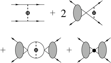
Figure 1: Relevant graphs contributing to charge independence breaking at leading order $\alpha\tilde{Q}^{-2}$. The blob stands for the resummation of the lowest order $(N^{\dagger}N)^{2}$ contact term $\sim C_{0}$. The open (filled) circle denotes a pion mass insertion $\sim\delta m^{2}$ (an insertion of the leading four–nucleon operators $\sim\alpha E_{0}^{(1)}$). For charge symmetry breaking, the leading contribution is given by the last diagram with the filled circle denoting an insertion $\sim\alpha E_{0}^{(2)}$.

$$\Delta{\cal A}^{II}_{1,-2} = \Gamma\left[\frac{1}{4p^{2}}\ln\left(1+\frac{4p^{2}}{m^{2}}\right)-\frac{1}{m^{2}+4p^{2}}\right]~{},$$

$$\Delta{\cal A}^{III}_{1,-2} = \Gamma\,{\cal F}\,\left[\frac{1}{pm}\arctan\frac{2p}{m}+\frac{i}{2pm}\ln\left(1++\frac{4p^{2}}{m^{2}}\right)-\frac{1+\frac{2ip}{m}}{m^{2}+4p^{2}}\right]$$

$$\Delta{\cal A}^{IV}_{1,-2} = \Gamma\,{\cal F}^{2}\left[\frac{i}{m^{2}}\arctan\frac{2p}{m}-\frac{1}{2m^{2}}\ln\left(\frac{m^{2}+4p^{2}}{\mu^{2}}\right)+\frac{1}{m^{2}}-\frac{1}{2}\frac{1+\frac{2ip}{m}}{m^{2}+4p^{2}}\right]$$

$$\Gamma = -\delta m^{2}\frac{g_{A}^{2}}{2f_{\pi}^{2}}~{},\quad{\cal F}=\left(\frac{mM{\cal A}_{-1}}{4\pi}\right)~{},\quad\delta m^{2}=m_{\pi^{\pm}}^{2}-m_{\pi^{0}}^{2}~{},$$ (16)

with ${\cal A}_{-1}\equiv{\cal A}_{0,-1}$ the leading term in the expansion of the $np$ ${}^{1}S_{0}$ amplitude,

$${\cal A}_{1}={C_{0}\over 1+{C_{0}M\over 4\pi}(\mu+ip)}~{}.$$ (17)

Furthermore, $f_{\pi}=92.4\,$MeV is the pion decay constant, $g_{A}=1.26$ the axial–vector coupling constant and $m^{2}=2m_{\pi^{\pm}}^{2}-m_{\pi^{0}}^{2}$ the “average” pion mass. The somewhat unusually looking expressions for $m^{2}$ and $\delta m^{2}$ are derived in appendix A. Note that while the diagrams II and III are convergent, IV diverges logarithmically. Therefore, the Lagrangian must contain a counterterm of the structure $E_{0}^{(1)}(\mu)\alpha(N^{\dagger}\tau^{3}N)(N^{\dagger}\tau^{3}N)$ to make the amplitude scale–independent. The leading CIB contribution thus scales as $\tilde{Q}^{-2}$ and for higher order operators with $2n$ derivatives we can establish the scaling property $E_{2n}^{(1)}\sim\tilde{Q}^{-2+n}$. This does not contradict the KSW power counting for the isospin symmetric theory since $\alpha\ll 1$. The insertion from this contact term is shown in the last diagram of fig. 1 and leads to an additional contribution to $\Delta{\cal A}$. In complete analogy, we can treat the leading order CSB effect which is due to an operator of the form $\alpha E_{0}^{(2)}(N^{\dagger}\tau_{3}N)(N^{\dagger}N)$. This term is, however, finite. Putting pieces together, this gives for the $nn$ and $pp$ case

$$\Delta{\cal A}^{VI}_{1,-2,{\rm nn}} = -\alpha\left(E_{0}^{(1)}-E_{0}^{(2)}\right)\left[\frac{{\cal A}_{-1}}{C_{0}}\right]^{2}~{},$$ (18)

$$\Delta{\cal A}^{VI}_{1,-2,{\rm pp}} = -\alpha\left(E_{0}^{(1)}+E_{0}^{(2)}\right)\left[\frac{{\cal A}_{-1}}{C_{0}}\right]^{2}~{},$$ (19)

where the coupling constants $E_{0}^{(1,2)}(\mu)$ obey the renormalization group equations,

$$\mu\,\alpha\,\frac{dE_{0}^{(1)}(\mu)}{d\mu} = \alpha\frac{M}{2\pi}E_{0}^{(1)}(\mu)C_{0}(\mu)\mu-\delta m^{2}\frac{Mg_{A}^{2}}{48\pi^{2}f_{\pi}^{2}}C_{0}^{2}(\mu)~{},$$

$$\mu\,\alpha\,\frac{dE_{0}^{(2)}(\mu)}{d\mu} = \alpha\frac{M}{2\pi}E_{0}^{(2)}(\mu)C_{0}(\mu)\mu~{}.$$ (20)

The relation of the $pp$ and $nn$ scattering lengths to the $np$ one reads (of course, in the $pp$ system Coulomb subtraction is assumed),

$$\frac{1}{a_{pp}} = \frac{1}{a_{np}}-\frac{4\pi\alpha(E_{0}^{(1)}+E_{0}^{(2)})}{MC_{0}^{2}}+\Delta~{},$$

$$\frac{1}{a_{nn}} = \frac{1}{a_{np}}-\frac{4\pi\alpha(E_{0}^{(1)}-E_{0}^{(2)})}{MC_{0}^{2}}+\Delta~{},$$ (21)

$$\Delta = \delta m^{2}\frac{g_{A}^{2}(-C_{0}M(m-2\mu)+8\pi+C_{0}Mm\ln(m^{2}/\mu^{2}))}{12\pi mC_{0}f_{\pi}^{2}}~{}.$$

For the effective ranges, we have only CIB

$$r_{nn}=r_{pp}=r_{np}+\delta m^{2}\frac{g_{A}^{2}(C_{0}M\mu+4\pi)(C_{0}M(3\mu-2m)+12\pi)}{6\pi Mm^{4}C_{0}^{2}f_{\pi}^{2}}~{}.$$ (22)

Note that the relations in eqs.(4,22) are perturbatively scale–independent and that the last one does not contain any unknown parameter. We remark that for the CIB scattering lengths difference the pion contribution alone is not scale–independent and can thus never be uniquely disentangled from the contact term contribution $\sim E_{0}^{(1)}$. While the leading OPE contribution resembles the result obtained in meson exchange models, the mandatory appearance of this contact term is a distinctively new feature of the effective field theory approach. Matters are somewhat different for CSB. Here, to leading order there is simply a four–nucleon contact term proportional to the constant $E_{0}^{(2)}$. Its value can be determined from a fit to the empirical value given in eq.(8). Corrections to the leading order CIB and CSB effect are classified below. We add the following remarks. Eqs.(4) and (22) are not exact but hold perturbatively. Similarly, the phase shifts are also defined perturbatively and therefore one can not have an exact effective range expansion of $\delta=\delta_{0}+\delta_{1}$ (referring to the isospin symmetric case for the moment). If one works e.g. at next–to–leading order, the norm of the S–matrix is not exactly one, $S^{\dagger}S=1+{\cal O}(\tilde{Q}^{2})\neq 1$. From this it follows that if one adjusts the parameters so as to reproduce the phase shifts in a certain momentum range, one can only approximately reproduce the scattering length and the effective range, $a\simeq a_{\rm exp}$ and $r\simeq r_{\rm exp}$, although the phase shifts may be very well described. This should be kept in mind.

We are now in the position to calculate the phase shifts. In total, we have five coupling constants, three of them related to the isospin–symmetric case, called $C_{0}$, $C_{2}$ and $D_{2}$. We fit the paramters $C_{0,2},D_{2}$ to the $np$ phase shift under the condition that the scattering length and effective range are exactly reproduced. The two new parameters $E_{0}^{(1,2)}$ are determined from the $nn$ and $pp$ scattering lengths. The resulting parameters at $\mu=m$ are of natural size,

$$C_{0} = -3.46~{}{\rm fm}^{2}~{},\quad C_{2}=2.75~{}{\rm fm}^{4}~{},\quad D_{2}=0.07~{}{\rm fm}^{4}~{},$$

$$E_{0}^{(1)} = -6.47~{}{\rm fm}^{2}~{},\quad E_{0}^{(2)}=1.10~{}{\rm fm}^{2}~{}.$$ (23)

The $np$ and $nn$ ${}^{1}S_{0}$ phase shifts are shown in fig. 2. To arrive at these curve, the physical masses for the proton and the neutron have been used. We stress again that the effect of the em terms $\sim E_{0}^{(1,2)}$ is small because of the explicit factor of $\alpha$ not shown in eq.(4). Having fixed these parameters, we can now predict the $nn$ ${}^{1}S_{0}$ phase shift as depicted by the solid line in fig.2. It agress with $nn$ phase shift extracted from the Argonne V18 potential (with the scattering length and effective range exactly reproduced) up to momemta of about 100 MeV. The analogous curve for the $pp$ system (not shown in the figure) is close to the solid line since the CSB effects are very small.

Figure 2: ${}^{1}S_{0}$ phase shifts for the $np$ (dashed line) and $nn$ (solid line) systems versus the nucleon cms momentum. The emipirical values for the $np$ case (open squares) are taken from the Nijmegen analysis. The open octagons are the $nn$ “data” based on the Argonne V18 potential.

5 Classification scheme

In the framework presented here, it is straightforward to work out the various leading (LO), next–to–leading (NLO) and next–to–next–to–leading order (NNLO) contributions to CIB and CSB, with respect to the expansion in $\tilde{Q}$, to leading order in $\alpha$ and the light quark mass difference. Here, I will simply enumerate the pertinent contributions which appear at a given order. This naturally also gives an estimate about their relative numerical importance based on simple dimensional analysis. Based on such an analysis, one can shed some light on the puzzles discussed in section 2, in particular the size of the $\pi\gamma$ graphs and the role of charge–dependent $\pi N$ coupling constants. Let me first consider CIB. In the classification scheme given below, TPE/3PE stands for two/three–pion–exchange.

LO	Pion mass difference in OPE,
$\alpha\tilde{Q}^{-2}$	four–nucleon contact interaction with no derivatives.
NLO	Pion mass difference in TPE,
$\alpha\tilde{Q}^{-1}$, $\varepsilon\tilde{Q}^{-1}$	four–nucleon contact interaction with two derivatives,
	insertions proportional to the $np$ mass difference,
NNLO	Pion mass difference in 3PE,
$\alpha\tilde{Q}^{0}$	four–nucleon contact interaction with four derivatives,
	CIB in the pion–nucleon coupling constants,
	$\pi\gamma$–exchange.

Note that there are no CIB effects due to the light quark mass difference linear in $\varepsilon=m_{u}-m_{d}$ from OPE and from the four–nucleon contact terms. These type of terms can only appear to second order in $\varepsilon$. Effects due to the charge dependence of the pion–nucleon coupling constants, i.e. isospin breaking terms from ${\cal L}_{\pi N}^{\rm em}$, only start to contribute at order $\alpha\tilde{Q}^{0}$. Such effects are therefore suppressed by two orders of $\tilde{Q}$ compared to the leading terms, i.e. by a numerical factor of about $(1/3)^{2}$. This finding is in agreement with the various numerical analyses performed in potential models (if one assumes that there is indeed some charge dependence in the pion–nucleon coupling constants, see e.g. the discussion in ref.[5].) We remark that the TPE contribution is nominally suppressed by one order in the small parameter, i.e. one would expect its contribution to be one third of the leading OPE with different pion masses. This agrees with some (but not all) meson–exchange model calculations.

Figure 3: $\pi\gamma$ graphs. For CIB, the leading contribution comes from the three diagrams a), b) and c). Due to the Kroll–Ruderman vertex in a) and c) the exchanged pion is charged. In case of CSB, the dominant contribution comes from b) with neutral pion exchange. c) vanishes due to parity and a) is suppressed by two additional powers in $\tilde{Q}$. Crossed graphs are not shown. Also omitted are the initial and final–state interactions between the nucleon.

Some remarks on the $\gamma\pi$ graphs (some of them shown in fig. 3) are in order. First, we note that their contribution for CIB is suppressed by two powers in $\tilde{Q}$ with respect to the leading terms (the power counting for these graphs is detailed in appendix B). The larger contribution found in some meson–exchange model calculations (approximately $1/3^{\rm rd}$ of the leading OPE contribution) is therefore at first sight at variance with dimensional analysis since one would expect a suppression of about $(1/3)^{2}$.[5] However, the much smaller value obtained in the more recent calculation of ref.[10] (performed in the static limit for the nucleons and Coulomb gauge for the photons), $\Delta a_{\rm CIB}(\pi\gamma)/\Delta a_{\rm CIB}({\rm OPE})\simeq-1/14.6$, is in much better agreement with the suppression by two powers in $\tilde{Q}$. This deserves further study. Second, the $\gamma\pi$ graphs evaluated in heavy baryon chiral perturbation theory have been used in a refined potential model calculation.[19] The ¹S₀ $np$ low–energy parameters were found to be very little affected. It is also instructive to see how the corrections due to the $np$ mass difference come about. For that, let us write the nucleon mass as $M+\delta M$, where $\delta M$ subsumes the em and strong contribution to the $np$ mass splitting, i.e. these terms are ${\cal O}(\alpha)$ and ${\cal O}(\varepsilon)$. Differentiating the leading isospin–symmertic amplitude eq.(17) with respect to the nucleon mass shift gives

$${\partial{\cal A}_{-1}\over\partial M}=-{{\cal A}_{-1}^{2}\over 4\pi}\,(\mu+ip)~{},$$ (24)

from which it follows that

$$\delta{\cal A}_{-1}=-\delta M{{\cal A}_{-1}^{2}\over 4\pi}\,(\mu+ip)\sim\varepsilon\tilde{Q}^{-1},\alpha\tilde{Q}^{-1}~{}.$$ (25)

We now turn to CSB. The pattern of the various contributions looks different:

LO	Electromagnetic four–nucleon contact interactions
$\alpha\tilde{Q}^{-2},\varepsilon Q^{-2}$	with no derivatives.
NLO	Em four–nucleon contact terms with two derivatives,
$\alpha\tilde{Q}^{-1},\varepsilon Q^{-1}$	strong isospin–breaking contact terms w/ two derivatives,
	insertions proportional to the $np$ mass difference.

We remark that the leading order CSB effects do not modify the effective range but the corresponding scattering length. Also, the leading $\pi\gamma$ graphs (with the exchanged pion now being neutral) are of order $\alpha\tilde{Q}^{0}$, i.e. suppressed by two orders in the KSW expansion parameter. This can be used as an argument to simply ignore such contributions in the study of CSB. Within meson–exchange models, their contribution comes out small but there seems to be no consensus about the actual size.[5] A similar hierarchy can also be derived based on the Weinberg power counting (which applies to the potential) as discussed in ref.[3].

6 The pionless theory

It is also of interest to consider a simplified theory in which even the pions are integrated out and one only deals with four–nucleon contact terms. Such an approximation is clearly only justifiable in a KSW–like approach as followed here. We do not want to enter the discussion about how to treat the pions (perturbative versus nonperturbative) but rather wish to see how accurate the pionless theory works for the question of isospin violation. In such an approach the connection to the chiral aspects of QCD is, of course, lost. Integrating out the pions modifies the coupling constants of the various contact terms like

EFT with pions:	$C_{0}$, $C_{2}$, $D_{2}$	and	$E_{0}^{(1)}$, $E_{0}^{(2)}$ ,
EFT without pions:	$\tilde{C}_{0}$, $\tilde{C}_{2}$	and	$\tilde{E}_{0}^{(1)}$, $\tilde{E}_{0}^{(2)}$ .

In the pionless theory, there is no more $D_{2}$ term. One has thus four parameters which can be fixed from the three scattering lengths and the $np$ effective range. The values of the parameters are

$$\tilde{C}_{0} = -3.42~{}{\rm fm}^{2}~{},\quad\tilde{C}_{2}=6.05~{}{\rm fm}^{4}~{},$$

$$\tilde{E}_{0}^{(1)} = 8.09~{}{\rm fm}^{2}~{},\quad\tilde{E}_{0}^{(2)}=1.07~{}{\rm fm}^{2}~{}.$$ (26)

Figure 4: ${}^{1}S_{0}$ phase shifts for the $np$ (dashed line) and $nn$ (solid line) systems versus the nucleon cms momentum in the pionless theory. The emipirical values for the $np$ case (open squares) are taken from the Nijmegen analysis.

Compared to the values for the theory with pions given in eq.(4), we note that the value of $\tilde{C}_{0}$ almost the same as the one of $C_{0}$. This is expected since we are close to a fix point. Noticeably, there is a dramatic difference in $\tilde{E}_{0}^{(1)}$ compared to $E_{0}^{(1)}$, which is also expected since the former pion contribution is now completely absorbed in the contact term. The resulting $np$ and $nn$ ${}^{1}S_{0}$ phase shifts shown in fig. 4. The description of the phase shifts has clearly worsened, they start to deviate from the data for momenta larger than 50 MeV and are considerably off the data for higher momenta, say about 200 MeV. These results are not surprising, but it is comforting to see that the pionless theory indeed describes the small momentum region correctly. For example, to this order the $nn$ effective range equals the one of the $np$ system which is in agreement with the data (partial wave analysis). However, the interpretation of the CIB is now very different since it is entirely given by the isospin–violating contact interaction. This makes a comparison with the results obtained in potential models very difficult, if not impossible.

7 Summary

We have shown that isospin violation can be systematically included in the effective field theory approach to the two–nucleon system in the KSW formulation. For that, one has to construct the most general effective Lagrangian containing virtual photons and extend the power counting accordingly. We have shown that this framework allows one to systematically classify the various contributions to charge indepedence and charge symmetry breaking (CIB and CSB). In particular, the power counting combined with dimensional analysis allows one to understand the suppression of contributions from a possible charge–dependence in the pion–nucleon coupling constants. Including the pions, the leading CIB breaking effects are the pion mass difference in OPE together with a four–nucleon contact term. These effects scale as $\alpha\tilde{Q}^{-2}$. Power counting lets one expect that the much debated contributions from two–pion exchange and $\pi\gamma$ graphs are suppressed by factors of $1/3$ and $(1/3)^{2}$, respectively. This is in agreement with some, but not all, previous more model–dependent calculations. The leading charge symmetry breaking is simply given by a four–nucleon contact term. One can also use the pionless theory to describe the observed CIB and CSB, but the physical interpretation is much less clear. It would certainly be interesting to investigate such effects in the presence of external sources.

Appendix A: The average pion mass

Here, I briefly show how the average pion mass used in the $np$ system in section 4 comes about. Consider the graphs shown in fig. 5. The strong interaction potential for OPE in the $nn$ and $pp$ system is given by the standard Yukawa form

$$V_{nn}=V_{pp}={g_{\pi N}^{2}\over 4\pi}{(\vec{\sigma}_{(1)}\cdot\vec{\nabla})(\vec{\sigma}_{(2)}\cdot\vec{\nabla})\over 4M^{2}}{{\rm e}^{-m_{0}r}\over r}~{},$$ (27)

where $m_{0}$ is a shorthand notation for the neutral pion mass.

Figure 5: OPE graphs for the $nn$ (left) and the $np$ system (middle and right).

For the $np$ case, we also have charged pion exchange,

$$V_{np}=V_{nn}\left[-1+2{\rm e}^{-\delta m\,r}\right]\simeq V_{nn}\left[1-2\delta m\,r\right]~{},$$ (28)

with $\delta m=m_{\pm}-m_{0}$ and $m_{\pm}$ denotes mass of the charged pion. So effectively one has for the $np$ OPE a mass

$$m=m_{0}+2\delta m\quad{\rm or}\quad m^{2}=m_{0}^{2}+2\delta m^{2}~{},$$ (29)

since $m^{2}\simeq m_{0}^{2}+4\delta m\,m_{0}=m_{0}^{2}+4(m_{\pm}-m_{0})m_{0}\simeq m_{0}^{2}+2\delta m^{2}$ (note that $\delta m^{2}\neq(\delta m)^{2}$). These are exactly the formulae used in section 4.

Appendix B: Power counting for the $\pi\gamma$ graphs

In this appendix, we will work out the explicit power counting of the various $\pi\gamma$–exchange diagrams (cf. fig. 3). First we need the counting rules for the propagators, vertices etc.: Pion propagator $\sim\tilde{Q}^{-2}$, nucleon propagator $\sim\tilde{Q}^{-1}$, pion-nucleon vertex $\sim\tilde{Q}$, photon-nucleon vertex $\sim\tilde{Q}^{0}$, charged pion-photon-nucleon vertex $\sim\tilde{Q}^{0}$, neutral pion-photon-nucleon vertex $\sim\tilde{Q}$ and loop integration $\sim\tilde{Q}^{4}$. This gives (displayed is the respective power in $\tilde{Q}$ for all vertices, propagators, etc for the specified diagram):

Graph	Vertices	Propagators	Loops	Total
3a ($\pi^{\pm}$)	0	-4	4	0
3a ($\pi^{0}$)	2	-4	4	2
3b ($\pi^{\pm}$)	2	-6	4	0
3b ($\pi^{0}$)	2	-6	4	0
3c ($\pi^{\pm}$)	1	-5	4	0
3c ($\pi^{0}$)	2	-5	4	1

For CIB, we have charged and neutral pion exchange and all $\pi\gamma$ diagrams 3a,b,c start contributing $\tilde{Q}^{0}$. In the case of CSB, matters are somewhat different. Graph 3b is leading at $\tilde{Q}^{0}$, while 3c is formally of order $\tilde{Q}$ but vanishes due to parity. The contribution of graph 3a to CSB is suppressed by two additional powers of the small momentum.

References

References

- [1] S. Weinberg, Nucl. Phys. B363 (1991) 3.
- [2] D.B. Kaplan, M.J. Savage and M.B. Wise, Phys. Lett. B424 (1999) 329; Nucl. Phys. B534 (1998) 329.
-
[3]
U. van Kolck, Ph.D. Thesis, University of Texas, Austin
(1993);
U. van Kolck, Few–Body Syst. Suppl. 9 (1995) 444. - [4] E. Epelbaum and Ulf-G. Meißner, nucl-th/9902042.
- [5] G.A. Miller, B.M.K. Nefkens and I. Slaus, Phys. Rep. 194 (1990) 1.
- [6] S.A. Coon, nucl-th/9903033.
- [7] V.G.J. Stoks et al., Phys. Rev. C49 (1994) 2950.
- [8] X. Kong and F. Ravndal, nucl-th/9811076.
- [9] B.R. Holstein, nucl-th/9901041.
- [10] J.L. Friar and S.A. Coon, Phys. Rev. C53 (1996) 588.
- [11] R. Urech, Nucl. Phys. B433 (1995) 234.
- [12] H. Neufeld and H. Rupertsberger, Z. Phys. C68 (195) 91.
- [13] Ulf-G. Meißner, G. Müller and S. Steininger, Phys. Lett. B406 (1997); (E) ibid B407 (1997) 434.
- [14] M. Knecht and R. Urech, Nucl. Phys. B519 (1998) 329.
- [15] Ulf-G. Meißner and S. Steininger, Phys. Lett. B419 (1998) 403.
- [16] G. Müller and Ulf-G. Meißner, hep-ph/9903375.
-
[17]
T. Mehen and I.W. Stewart, Phys. Lett. B445 (1999) 378;
nucl-th/9809095. - [18] D.B. Kaplan, nucl-th/9901003.
- [19] U. van Kolck et al., Phys. Rev. Lett. 80 (1998) 4386.