Kinetic freeze out models

Abstract

Freeze out of particles across a space-time hypersurface is discussed in kinetic models. The calculation of final momentum distribution of emitted particles is described for freeze out surfaces, with spacelike normals. The resulting non-equilibrium distribution does not resemble, the previously proposed, cut Jüttner distribution, and shows non-exponential $p_{t}$-spectra similar to the ones observed in experiments.

1. Introduction

Continuum and fluid dynamical models, due to their simplicity are very popular in heavy ion physics, because they connect directly collective macroscopic matter properties, like the Equation of State (EoS) or transport properties, to measurables.

In contrast to kinetic, Monte Carlo models, in continuum models the evaluation of measurables is a problem in itself. Particles, which leave the system and reach the detectors, can be taken into account via source (drain) terms in the 4-dimensional space-time based on kinetic considerations, or in a more simplified way via freeze out (FO) or final break-up schemes, where the frozen out particles are formed on a 3-dimensional hypersurface in space-time. Such freeze out descriptions are important ingredients of evaluations of two-particle correlation data, transverse-, longitudinal-, radial-, and cylindrical- flow analyses, transverse momentum and transverse mass spectra and many other observables.

The general theory of discontinuities in relativistic flow was not worked out for a long time, and the 1948 work of A. Taub [1] discussed discontinuities across propagating hypersurfaces only (which have a spacelike unit normal vector $d\hat{\sigma}^{\mu}$, $d\hat{\sigma}^{\mu}d\hat{\sigma}_{\mu}=-1$). Events happening on a propagating, (2 dimensional) surface belong to this category.

Another type of change in a continuum is an overall sudden change in a finite volume. This is represented by a hypersurface with a timelike normal ($d\hat{\sigma}^{\mu}d\hat{\sigma}_{\mu}=+1$). If one applies Taub’s formalism to freeze out surfaces with timelike normal vectors, one gets a usual Taub adiabat, but the equation of the Rayleigh line will yield imaginary values for the particle current across the front. Only in 1987 Taub’s approach was generalized to both types of surfaces [2], making it possible to take into account conservation laws exactly across any surface of discontinuity in relativistic flow. This approach also eliminates the imaginary particle currents arising from the equation of the Rayleigh line. When the EoS is different on the two sides of the FO front these conservation laws yield changing temperature, density, flow velocity across the front. Based on conservation laws and on simple kinetic considerations the idealized surface freeze out models were completely worked out in refs. [3, 4, 6, 5].

2. Conservation laws across idealized freeze out fronts

The FO hypersurface is an idealization of a layer of finite thickness (of the order of a mean free path or collision time) where the frozen-out particles are formed and the interactions in the matter become negligible. The dynamics of this layer can be described in different kinetic models as Monte Carlo models [9, 10] or four-volume emission models [11, 12, 13, 14, 15]. The zero thickness limit of such a layer is the idealized FO surface. Kinetic models for hadronic degrees of freedom indicate that such an idealization is meaningful only for collisions of massive heavy ions like Au+Au or Pb+Pb [9, 10]. If we include quark-gluon plasma in our reaction model with rapid final hadronization which coincides with freeze out [16, 17], the applicability of idealized surface freeze out description becomes even better.

In general the energy - momentum tensor changes discontinuously across this idealized hypersurface. If the flow is not orthogonal to this surface the four-vector of the flow velocity will also change across this surface [2, 16, 18]. The FO discontinuity has a timelike normal in most cases, and so the method for the description of timelike detonations and deflagrations [2] should be used (see also [16, 18, 19, 20, 21]).

If $d\sigma^{\mu}$ is the normal vector of an element of the FO hypersurface ($d\hat{\sigma}^{\mu}$ is a unit vector parallel to $d\sigma^{\mu}$), the observable triple differential cross section is obtained by integrating the FO current over the whole FO hypersurface. This is described by the Cooper-Frye formula [3, 6]:

$$E\frac{dN}{d^{3}p}=\int f_{FO}(x,p;T,n,u^{\nu})\ p^{\mu}d\sigma_{\mu}\ ,$$ (1)

where $f_{FO}(x,p;T,n,u^{\nu})$ is the post FO phase space distribution of frozen out particles which is not known from the fluid dynamical model. When we apply this formula we have to ensure [6] that: (i) the particles are really leaving the surface outwards:

$$f_{FO}(x,p;T,n,u^{\nu})=\Theta(p^{\mu}\ d\hat{\sigma}_{\mu})f_{FO}(x,p;T,n,u^{\nu})\,,$$ (2)

and (ii) the conservation laws and entropy condition are satisfied [1, 2]:

$$[N^{\mu}\ d\hat{\sigma}_{\mu}]=0\,,\ \ \ \ \ \ [T^{\mu\nu}\ d\hat{\sigma}_{\mu}]=0\ \ \ \ \ {\rm and}\ \ \ \ \ \ [S^{\mu}\ d\hat{\sigma}_{\mu}]\geq 0\,,\ \ \ \ \ \$$ (3)

where $[A]\equiv A-A_{0}$, and the pre FO baryon and entropy currents and energy-momentum tensor are $N_{0}^{\mu}$, $S_{0}^{\mu}$ and $T_{0}^{\mu\nu}$, while the post freeze out quantities are, $N^{\mu}$ $S^{\mu}$ and $T^{\mu\nu}$, In numerical calculations the local freeze out surface can be determined most accurately via self-consistent iteration [4, 22]. This fixes the parameters of our post FO momentum distribution, $f_{FO}(x,p;T,n,u^{\nu})$ if the shape of the distribution is known.

A simple approach is to assume that $f_{FO}$ is a cut Jüttner distribution [4, 6] if we have a FO hypersurface with spacelike normal. It was shown that one can formally solve the freeze out problem with this ansatz [6].

3. Freeze out distribution from kinetic theory

At the same time in a kinetic gas model it was studied how we can obtain a non-equilibrium post FO distribution across a FO hypersurface with a spacelike normal [5]. The result indicated that actually the cut Jüttner distribution is not a realistic choice. Apart of the non-physical shape by the sharp momentum cut, the simplified model which recovered the cut Jüttner shape led to other nonphysical consequences also: The freeze out was not complete in the model even for an asymptotically large thickness of the FO layer. Thus, the simple kinetic model [5] had two unsatisfactory features: (i) it did not achieve complete freeze out, and (ii) it resulted in exponentially weakening freeze out with a FO layer thickness which tends to infinity. A solution to the first problem has also been suggested.

Here we present solutions to both problems by making additional improvements of the model used in [5]. The two extended models are still very superficial and should not be considered as final and physically realistic solutions of the freeze out problem. For transparency we perform and demonstrate the modifications separately, although both of these could be included in a combined model. This way we can see which improvement (consideration of which physical process) cures problems.

Let us assume an infinitely long tube with its left half ($x<0$) filled with nuclear matter and in the right vacuum is maintained. We can remove the dividing wall at $t=0$, and then the matter will expand into the vacuum. By continuously removing particles at the right end of the tube and supplying particles on the left end, we can establish a stationary flow in the tube, where the particles will gradually freeze out in an exponential rarefaction wave propagating to the left in the matter. We can move with this rarefaction wave or front, so that we describe it from the reference frame of the front (RFF), where the rarefaction is stationary.

In this frame, we have a stationary supply of equilibrated matter from the left, and a stationary rarefaction front on the right, $x>0$. We can describe the freeze out kinetics on the r.h.s. of the tube assuming that we have two components of our momentum distribution [12, 13, 14], $f_{free}(x,\vec{p})$ and $f_{int}(x,\vec{p})$. However, we only assume that at $x=0$, $f_{free}$ vanishes exactly and $f_{int}$ is an ideal Jüttner distribution (supplied by the inflow of equilibrated matter), while $f_{int}$ gradually disappears and $f_{free}$ gradually builds up as $x$ tends to infinity.

Let us recall [5] the most simple kinetic model describing the evolution of such a system. Starting from a fully equilibrated Jüttner distribution the two components of the momentum distribution develop according to the coupled differential equations:

$$\partial_{x}f_{int}(x,\vec{p})dx = -\Theta(p^{\mu}d\hat{\sigma}_{\mu})\frac{\cos\theta_{\vec{p}}}{\lambda}f_{int}(x,\vec{p})dx,\$$

$$\partial_{x}f_{free}(x,\vec{p})dx = +\Theta(p^{\mu}d\hat{\sigma}_{\mu})\frac{\cos\theta_{\vec{p}}}{\lambda}f_{int}(x,\vec{p})dx.$$ (4)

Here $\cos\theta_{\vec{P}}=\frac{p_{x}}{p}$ in the RFF frame. The interacting component, $f_{int}$, will deviate from the Jüttner shape and the solution will take the form:

$$f_{int}(x,\vec{p})=f_{Juttner}(x=0,\vec{p})\exp\left[-\Theta(p^{\mu}d\hat{\sigma}_{\mu})\frac{\cos\theta_{\vec{p}}}{\lambda}x\right].$$ (5)

This solution is depleted in the forward $\vec{p}$-direction, particularly along the $x$-axis. Inserting it into the second differential equation above, leads to the freeze out solution:

$$f_{free}(x,\vec{p})=f_{Juttner}(x=0,\vec{p})\left\{1-\exp\left[-\Theta(p^{\mu}d\hat{\sigma}_{\mu})\frac{\cos\theta_{\vec{p}}}{\lambda}x\right]\right\}=$$

(6)

$$f_{Juttner}(x=0,\vec{p})-f_{int}(x,\vec{p})\,.$$

At $x\longrightarrow\infty$ this distribution will tend to the cut Jüttner distribution introduced in the previous section. The remainder of the original Jüttner distribution survives as $f_{int}$, even if $x\longrightarrow\infty$. In this model the particle density does not change with $x$, barely particles moving faster than the freeze out front (i.e. $p^{\mu}d\hat{\sigma}_{\mu}>0$) are transferred gradually from component $f_{int}$ to component $f_{free}$. This is a highly unrealistic model, indicating that rescattering and re-thermalization should be taken into account in $f_{int}$. This would allow particle transfer from the ”negative momentum part” (i.e. $p^{\mu}d\hat{\sigma}_{\mu}<0$) of $f_{int}$ to $f_{free}$, which is not possible otherwise.

4. Freeze out distribution with rescattering

The assumption that the interacting part of the distribution remains the distorted (after some drain) Jüttner distribution, is of course highly unrealistic. As suggested in ref. [5] rescattering within this component will lead to re-thermalization and re-equilibration of this component. Thus the evolution of the component, $f_{int}$ is determined by drain terms as much as the re-equilibration. Here, we repeat the introduction of the model with rescattering, and present it more generally for both positive and negative flow parameter velocities. This turned out necessary because during the FO process the interacting component will acquire negative velocity parameters, even with large positive initial velocities. We also introduce the $m=0$ limit of the suggested solution which enables us to present a transparent and not completely numerical solution.

If we include the collision terms explicitly into the transport equations (4) in general case leads to a combined set of integro-differential equations. We can, however, take advantage of the relaxation time approximation to simplify the description of the dynamics.

Then the two components of the momentum distribution develop according to the coupled differential equations:

$$\begin{array}[]{rll}\partial_{x}f_{int}(x,\vec{p})dx=&-\Theta(p^{\mu}d\hat{\sigma}_{\mu})\frac{\cos\theta_{\vec{p}}}{\lambda}f_{int}(x,\vec{p})dx+\\ &&\\ &+\left[f_{eq}(x,\vec{p})-f_{int}(x,\vec{p})\right]\frac{1}{\lambda^{\prime}}dx,\end{array}$$ (7)

$$\begin{array}[]{rll}\partial_{x}f_{free}(x,\vec{p})dx=&+\Theta(p^{\mu}d\hat{\sigma}_{\mu})\frac{\cos\theta_{\vec{p}}}{\lambda}f_{int}(x,\vec{p})dx.\end{array}$$ (8)

The interacting component of the momentum distribution, described by eq. (7), shows the tendency to approach an equilibrated distribution with a relaxation length $\lambda^{\prime}$. Of course due to the energy, momentum and conserved particle drain, this distribution, $f_{eq}(x,\vec{p})$ is not the same as the initial Jüttner distribution, but its parameters, $n_{eq}(x)$, $T_{eq}(x)$ and $u^{\mu}_{eq}(x)$, change as required by the conservation laws.

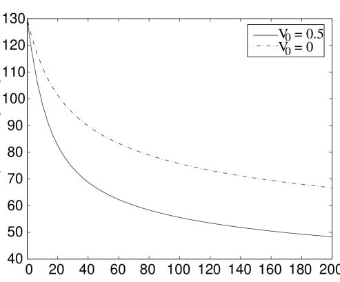
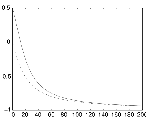
Fig. 1.: The temperature and flow velocity of the interacting component in the rest frame of the freeze out front (RFF) for baryonfree and massless gas, calculated according to the coupled set of equations (4.1.). We assume an initial temperature of $T_{0}=130$ MeV to fit the situation in refs. [16, 17].

Conservation Laws.   In this case the change of the conserved quantities caused by the particle transfer from component $int$ to component $free$ can be obtained in terms of the distribution functions as:

$$dN_{i}^{\mu}=-\frac{dx}{\lambda}\int\frac{d^{3}p}{p_{0}}p^{\mu}\Theta(p^{\mu}d\hat{\sigma}_{\mu})\cos\theta_{\vec{p}}f_{int}(x,\vec{p})$$ (9)

and

$$dT_{i}^{\mu\nu}=-\frac{dx}{\lambda}\int\frac{d^{3}p}{p_{0}}p^{\mu}p^{\nu}\Theta(p^{\mu}d\hat{\sigma}_{\mu})\cos\theta_{\vec{p}}f_{int}(x,\vec{p}).$$ (10)

If we do not have collision or relaxation terms in our transport equation then the conservation laws are trivially satisfied. If, however, collision or relaxation terms are present, these contribute to the change of $T^{\mu\nu}$ and $N^{\mu}$, and this should be considered in the modified distribution function $f_{int}(x,\vec{p})$.

4.1. Immediate re-thermalization limit

We can get from the equation (7) the general solution for $f_{int}(x,\vec{p})$ in the RFF frame:

$$f_{int}(x,\vec{p})=e^{-\frac{x}{\lambda}[\Theta(p^{x})\frac{p^{x}}{p}+\frac{\lambda}{\lambda^{\prime}}]}\left\{f_{int}(0,\vec{p})+\phantom{\int_{0}^{x}e^{\frac{x}{x}}}\right.$$

$$\left.+\frac{1}{\lambda^{\prime}}\int_{0}^{x}f_{eq}(x^{\prime},\vec{p})e^{\frac{x^{\prime}}{\lambda}[\Theta(p^{x})\frac{p^{x}}{p}+\frac{\lambda}{\lambda^{\prime}}]}dx^{\prime}\right\}\,.$$ (11)

As a first approximation to this solution let us assume that $\lambda^{\prime}\ll\lambda$, i.e. re-thermalization is much faster than particles freezing out, or much faster than parameters, $n_{eq}(x)$, $T_{eq}(x)$ and $u^{\mu}_{eq}(x)$ change. Eq. (11) then leads to

$$f_{int}(x,\vec{p})\approx f_{eq}(x,\vec{p}),\ \ {\rm for}\ \ \lambda^{\prime}\ll\lambda\,.$$ (12)

For $f_{eq}(x,\vec{p})$ we can assume the spherical Jüttner form at any $x$ including both positive and negative momentum parts with parameters $\hat{n}(x),\ T(x)$ and $u_{RFG}^{\mu}(x)$, where $u_{RFG}^{\mu}(x)$ is the peak velocity of the Jüttner gas (which is the same as the flow velocity of the non-cut Jüttner gas), and $\hat{n}(x)$ is the proper density i.e. the density in the frame moving with $u_{RFG}^{\mu}(x)$ [6, 5].

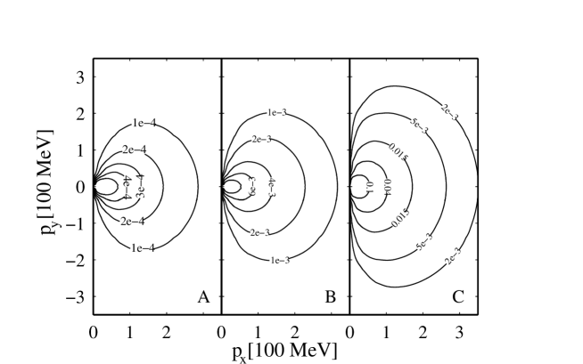
Fig. 2.: The freeze-out distribution, $f_{free}(x,\vec{p})$, in the rest frame of the freeze out front (RFF) calculated according to eqs. (4.1.). A, B and C correspond to $x=0.2\lambda,\ 3\lambda,\ 100\lambda$ respectively and $u_{RFG}^{\mu}|_{x=0}=(1,0,0,0)$. The numbers in the contours are in arbitrary units. The distribution is asymmetric and elongated in the freeze out direction, $x$. This may lead to a large-$p_{t}$ enhancement, compared to the usual Jüttner assumption used in most previous calculations as a freeze out distribution. Note that $f_{int}(x,\vec{p})$ does not tend to the cut Jüttner distribution in the limit $x\rightarrow\infty$.

In this case the change of conserved quantities due to particle drain or transfer can be evaluated for an infinitesimal $dx$. We assume that the 3-flow is normal to the freeze out surface. The changes of the conserved particle currents and energy-momentum tensor in the RFF, using the notation of ref. [6],^b eqs. (9,10) are given by

$$\begin{array}[]{rll}dN_{i}^{0}=&-\frac{dx}{\lambda}\frac{\tilde{n}}{4v^{2}\gamma^{2}}\left\{aK_{1}(b)+jb(3v^{2}-1)\gamma^{2}[(1+j)K_{1}(a)-{\cal K}_{1}(a,b)]\right.\\ &&\\ &\left.+j\gamma v^{2}b^{2}[(1+j)K_{0}(a)-{\cal K}_{0}(a,b)]+2jv^{3}\gamma^{3}(b+1)e^{-b}\right\}\\ &&\\ \stackrel{{\scriptstyle\scriptscriptstyle m=0}}{{\longrightarrow}}&-\frac{dx}{\lambda}\frac{\tilde{n}}{4}\gamma(1+u)^{2},\\ &&\\ dN_{i}^{x}=&-\frac{dx}{\lambda}\frac{\tilde{n}}{4jv^{3}\gamma^{3}}\left\{-2K_{0}(b)+2jv\gamma^{2}e^{-b}[v^{2}\gamma^{2}(b+1)-v^{2}b-1]\right.\\ &&\\ &\left.+j(2+v^{4}\gamma^{2}b^{2})[(1+j)K_{0}(a)-{\cal K}_{0}(a,b)]\right.+\\ &&\\ &\left.+jv^{2}(3v^{2}-1)\gamma^{3}b[(1+j)K_{1}(a)-{\cal K}_{1}(a,b)]\right\}\\ &&\\ \stackrel{{\scriptstyle\scriptscriptstyle m=0}}{{\longrightarrow}}&-\frac{dx}{\lambda}\frac{\tilde{n}}{4u^{3}\gamma^{3}}\left[-2u\gamma^{2}(1+u)-2ln(1-u)+u^{2}\gamma^{4}(1+u)^{2}\right],\end{array}$$

and by the expressions

$$\begin{array}[]{rll}dT_{i}^{00}=&-\frac{dx}{\lambda}\frac{\tilde{n}T}{4v^{2}\gamma^{2}}\left\{\frac{a}{\gamma}K_{1}(b)+jv\gamma^{2}e^{-b}\!\left[(1{+}3v^{2})\gamma^{2}\!A(b)-\right.\right.\\ &&\\ &\left.-(2+v^{2}b^{2})(b+1)+v^{4}(1+\frac{v^{2}}{3})\gamma^{2}b^{3}\right]+a^{2}K_{0}(b)\\ &&\\ &+jv^{2}\gamma^{2}b^{2}(3+v^{2})\left[(1+j)K_{2}(a)-{\cal K}_{2}(a,b)\right]\\ &&\\ &+j(v^{2}b^{2}-v^{2}-1)\gamma b\left[(1+j)K_{1}(a)-{\cal K}_{1}(a,b)\right]\\ &&\\ &\left.-jb^{2}\left[(1+j)K_{0}(a)-{\cal K}_{0}(a,b)\right]\right\}\\ &&\\ \stackrel{{\scriptstyle\scriptscriptstyle m=0}}{{\longrightarrow}}&-\frac{dx}{\lambda}\frac{\tilde{n}T}{4u^{2}\gamma^{2}}\left[1-u^{2}+2u\gamma^{4}(1+u)^{3}-\gamma^{2}(1+u)^{2}\right]\ ,\\ &&\\ dT_{i}^{0x}=&-\frac{dx}{\lambda}\frac{\tilde{n}T}{4jv^{3}\gamma^{3}}\left\{j(1+3v^{2})v^{2}\gamma^{3}b^{2}\left[(1+j)K_{2}(a)-{\cal K}_{2}(a,b)\right]\right.\\ &&\\ &+jv^{2}\gamma^{5}e^{-b}\left[v(v^{2}+3)A(b)-a^{2}bv^{3}+(1+3v^{2})\frac{(bv)^{3}}{3}-va^{2}\right]\\ &&\\ &\left.+jv^{4}\gamma^{2}b^{3}\left[(1+j)K_{1}(a)-{\cal K}_{1}(a,b)\right]\right\}-\frac{2T}{jv\gamma}dN_{i}^{0}\\ &&\\ \stackrel{{\scriptstyle\scriptscriptstyle m=0}}{{\longrightarrow}}&-\frac{dx}{\lambda}\frac{\tilde{n}T}{2}\gamma^{2}(1+u)^{3}\ ,\\ &&\\ dT_{i}^{xx}=&-\frac{dx}{\lambda}\frac{\tilde{n}T}{4v^{4}\gamma^{4}}\left\{jv^{4}(3+v^{2})\gamma^{4}b^{2}\left[(1+j)K_{2}(a)-{\cal K}_{2}(a,b)\right]\right.\\ &&\\ &+jv^{6}\gamma^{3}b^{3}\left[(j+1)K_{1}(a)-{\cal K}_{1}(a,b)\right]+jv^{3}\gamma^{6}e^{-b}\\ &&\\ &\left.\left[\frac{v(3+v^{2})(bv)^{3}}{3}+a^{2}(v^{4}b-1)+(3v^{2}+1)A(b)\right]\right\}-\frac{3T}{jv\gamma}dN_{i}^{x}\\ &&\\ \stackrel{{\scriptstyle\scriptscriptstyle m=0}}{{\longrightarrow}}&-\frac{dx}{\lambda}\frac{\tilde{n}T}{4u^{4}\gamma^{4}}\left[2u^{3}\gamma^{6}(1+u)^{3}-3u^{2}\gamma^{4}(1+u)^{2}+\right.\\ &&\\ &\left.+6u\gamma^{2}(1+u)+6ln(1-u)\right]\ ,\\ &&\\ dT_{i}^{yy}=&-\frac{dx}{\lambda}\frac{\tilde{n}T}{8v^{4}\gamma^{4}}\left\{-jv^{2}\gamma^{3}(v^{2}+1)b\left[(1+j)K_{1}(a)-{\cal K}_{1}(a,b)\right]\right.\\ &&\\ &-jv^{4}\gamma^{2}b^{2}\left[(1+j)K_{0}(a){-}{\cal K}_{0}(a,b)\right]+bv^{2}K_{1}(b)\\ &&\\ &\left.-2jv^{3}\gamma^{4}(b{+}1)e^{-b}\right\}+\frac{3T}{2jv\gamma}dN_{i}^{x}\par\\ &&\\ \stackrel{{\scriptstyle\scriptscriptstyle m=0}}{{\longrightarrow}}&-\frac{dx}{\lambda}\frac{\tilde{n}T}{8u^{4}\gamma^{4}}\left[2u^{2}\gamma^{4}(1{+}u)^{2}-6u\gamma^{2}(1{+}u)+u^{2}-2ln(1{-}u)\right],\end{array}$$

and $dT_{i}^{zz}=dT_{i}^{yy}$. Note that in RFF the flow velocity of the re-thermalized component is $u_{i,RFG}^{\mu}(x)=\gamma(x)\ (1,u(x),0,0)|_{RFF}$, where $\gamma=1/\sqrt{1-u^{2}}$; and we also use the notation $v=|u|$ and $j=sgn(u)$.

The new parameters of distribution $f_{int}$, after moving to the right by $dx$ can be obtained from $dN_{i}^{\mu}$ and $dT_{i}^{\mu\nu}$. The conserved particle density of the re-thermalized spherical Jüttner distribution after a step $dx$ is:

$$\hat{n}_{i}(x+dx)=\hat{n}_{i}(x)+d\hat{n}_{i}(x)=\sqrt{N_{i}^{\mu}(x+dx)N_{i,\mu}(x+dx)}\ ,$$

where the expressions are invariant scalars. The differential equation describing the change of the proper particle density is:

$$d\hat{n}_{i}(x)=u_{i,RFG}^{\mu}(x)\ dN_{i,\mu}(x)\,.$$ (13)

Although this covariant equation is valid in any frame, we can calculate it in the RFF, where the values of $dN_{i}^{\mu}$ were given above in eq. (4.1.).

For the re-thermalized interacting component Eckart’s flow velocity is the velocity of the RFG, which changes with $x$, so we denote this frame as RFG$(x)$. The velocity of this frame decreases with decreasing $x$ due to the particle drain at positive momenta. For the spherical Jüttner distribution the Landau and Eckart flow velocities are the same, $u^{\mu}_{i,E,RFG}(x)=u^{\mu}_{i,L,RFG}(x)=u^{\mu}_{i,RFG}(x)$. Thus we can evaluate the flow velocity $u_{i,RFG}^{\mu}(x+dx)$:

$$u^{\mu}_{i,RFG}(x+dx)=N_{i}^{\mu}(x+dx)/\sqrt{N_{i}^{\mu}N_{i,\mu}}\,,$$

which leads to the following covariant expression

$$du^{\mu}_{i,E,RFG}(x)=\Delta^{\mu\nu}_{i}(x)\ \frac{dN_{i,\nu}(x)}{\hat{n}_{i}(x)}\,,$$ (14)

where $\Delta^{\mu\nu}_{i}(x)=g^{\mu\nu}-u_{i,RFG}^{\mu}(x)\,u_{i,RFG}^{\nu}(x)\,$  is a projector to the plane orthogonal to $u^{\mu}_{i,RFG}(x)$. This equation is valid in any reference frame, nevertheless we know the four-vectors on the r.h.s. in the RFF explicitly. Then the new Eckart flow velocity of the matter is $u^{\mu}_{i,E,RFG}(x+dx)$ $=$ $u^{\mu}_{i,RFG}(x)$ $+$ $du_{i,E,RFG}^{\mu}(x)$.

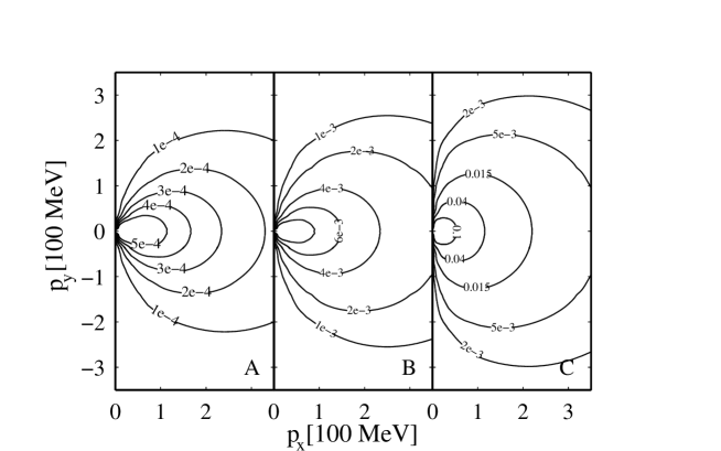
Fig. 3.: The same as Fig. 2, just $u_{RFG}^{\mu}|_{x=0}=\gamma(1,0.5,0,0)$. We can see that particles are freezing out faster if we start with positive initial flow velocity.

To get the temperature and the change of Landau’s flow velocity, we analyze the change of the energy momentum tensor. Before the particle drain the energy - momentum tensor at $x$ in the RFG is diagonal, $T^{\mu\nu}_{i}(x)={\rm diag}(e_{i},P_{i},P_{i},P_{i})|_{RFG(x)}$ while in the RFF $T^{\mu\nu}_{i}(x)$ $=$ $\left[(e_{i}+P_{i})\right.$ $u_{i,RFG}^{\mu}u_{i,RFG}^{\nu}(x)$ $\left.-P_{i}g^{\mu\nu}\right]|_{RFF(x)}$. Adding to this the drain terms, $dT^{\mu\nu}_{i}(x)$, arising from the freeze out while we move to the right by $dx$, yields $T^{\mu\nu}_{i}(x+dx)$ which will not be diagonal in the RFG$(x)$ and the pressure part will not be isotropic. We can Lorentz transform this to another frame which diagonalizes $T^{\mu\nu}_{i}(x+dx)$. This means to find the Landau flow velocity of the new system, $u^{\mu}_{i,L,RFG}(x+dx)$ in the original RFG$(x)$. After a straightforward diagonalization, a somewhat tricky algebra and neglecting second and higher order terms we arrive at the covariant expression[5]

$$du^{\mu}_{i,L,RFG}(x)=\frac{\Delta^{\mu\nu}_{i}(x)\ \ dT_{i,\nu\sigma}\ \ u^{\sigma}_{i,RFG}(x)}{e_{i}+P_{i}}.$$ (15)

Although, for the spherical Jüttner distribution the Landau and Eckart flow velocities are the same, the change of this flow velocity calculated from the baryon current and from the energy current are different in general

$$du^{\mu}_{i,E,RFG}(x)\neq du^{\mu}_{i,L,RFG}(x)\,.$$

This is a clear consequence of the asymmetry caused by the freeze out process as it was discussed in ref. [5].

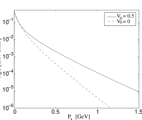
Fig. 4.: The local transverse momentum (here $p_{x}$) distribution for baryon free, massless gas at $p_{y}=0$, $x=100\lambda$ and $T_{0}=130\,$MeV. The transverse momentum spectrum is obviously curved due to the freeze out process, particularly for large initial flow velocities. The apparent slope parameter increases with increasing transverse momentum. This behavior agrees with observed pion transverse mass spectra at SPS [24, 25].

In the special case of the massless limit we can calculate $du^{\mu}_{i,E,RFG}(x)$ and $du^{\mu}_{i,L,RFG}(x)$ in the RFG. In this frame $u^{\mu}_{i}=(1,0,0,0)$, and according to (14) and (15) we can get: $du^{0}_{i,E}=du^{0}_{i,L}=0$, $du^{y}_{i,E}=du^{y}_{i,L}=0$, $du^{z}_{i,E}=du^{z}_{i,L}=0$ and

$$du^{x}_{i,E}=\frac{dN^{x}_{i}}{n}=\frac{dN^{x}_{i}}{N^{0}_{i}}$$

$$du^{x}_{i,L}=\frac{dT^{x0}_{i}}{e+P}=\frac{dT^{x0}_{i}}{T^{00}_{i}+T^{xx}_{i}}.$$

Here the last values of both equations are in the RFG. Thus we can see that $du^{x}_{i,E}={4\over 3}du^{x}_{i,L}\,,$ in the massless limit. Using the definitions of the $dN^{x}$ and $dT^{x0}$ from equations (9),(10) and $N^{0}$ and $T^{00}$ from section 2.   , it is easy to see, that in the limit $m\rightarrow 0$, (and $p^{0}=p$) the calculation leads to the integral:

$$du^{x}_{i,E}={4\over 3}du^{x}_{i,L}=-\frac{dx}{2\lambda}\int_{-1}^{1}d\cos\theta\ \ \frac{\cos\theta(\cos\theta-u)}{1-u\cos\theta}\Theta(u-\cos\theta)\,,$$

where $u$ is defined via $u_{i,RFG}^{\mu}=\gamma(x)(1,u,0,0)$ (in RFF), and $\cos\theta$ is the polar angle of the emitted particle in the RFG. (The polar emission angle in RFF, given earlier, can be expressed as $\cos\theta_{\vec{p}}=(\cos\theta-u)/(1-u\cos\theta)\,.$)

This problem does not occur for the freeze out of baryonfree plasma, and we have only $du^{\mu}_{i,L}$.

The last item is to determine the change of the temperature parameter of $f_{int}$. From the relation $e\equiv u_{\mu}T^{\mu\nu}u_{\nu}$ we readily obtain the expression for the change of energy density

$$de_{i}(x)=u_{\mu,i,RFG}(x)\ dT^{\mu\nu}_{i}(x)\ u_{\nu,i,RFG}(x)\,,$$ (16)

and from the relation between the energy density and the temperature (e.g. Chapter 3 in ref. [7]), we can obtain the new temperature at $x+dx$. Fixing these parameters we fully determined the spherical Jüttner approximation for $f_{int}$.

The application of this model to the baryonfree and massless gas gives the following coupled set of equations:

$$\frac{d\ln{T}}{dx}=-\frac{u_{\mu}\tau^{\mu\nu}u_{\nu}}{4\sigma_{SB}}\,,$$

(17)

$$\frac{du^{\mu}}{dx}=-\frac{3}{4\sigma_{SB}}\left[\tau^{\mu\nu}-u^{\mu}u_{\sigma}\tau^{\sigma\nu}\right]u_{\nu}\,.$$

Here we use the EoS, $e=\sigma_{SB}T^{4}$,  and the definition $dT^{\mu\nu}$ $=$ $-dx\,\tau^{\mu\nu}T^{4}$,  where $dT^{\mu\nu}$ are given by eqs. (4.1.), and so $x$ is measured in units of $\lambda$.

The results of numerical calculation are displayed in Figs. 1 - 4. The velocity and temperature of the interacting component are gradually decreasing due to the loss of particles carrying most momentum and thermal energy. Thus, we see that $T\rightarrow 0$, when $x\rightarrow\infty$. So, $f_{int}(x,\vec{p})=\frac{1}{(2\pi\hbar)^{3}}\exp[(\mu-p^{\nu}u_{\nu})/T]\rightarrow 0$, when $x\rightarrow\infty$. Thus, all particles freeze out in the model with rescattering.

Now we can find the distribution function for the noninteracting, frozen out part of particles according to equation (8). The results are shown in Fig. 2 - Fig. 4. We would like to note that now $f_{free}(x,\vec{p})$ does not tend to the cut Jüttner distribution in the limit $x\rightarrow\infty$, it has a smooth, anisotropic shape. Most importantly the slope in the FO direction is not exponential, resembling recent experimental data.

5. Volume emission model

In this section we demonstrate an improvement which yields complete FO in a layer of finite width. We calculate the kinetic freeze out distribution based on four volume emission models [12, 13, 14]. In order to illustrate the physical mechanism of this freeze out process, let us study again a simple one-dimensional flow [6, 5]. We suppose an infinite tube where a stationary flow of a fluid is supplied from the left ($x<0$), so that the freeze out occurs for the positive direction of $x$.

In the four volume emission model, we introduce the basic quantity, the so-called escape probability

$${\cal P}(\vec{r},t,\vec{p})\equiv e^{-\int_{t}^{\infty}\sigma v_{rel}{\sf n}(\vec{r}+\vec{v}t,t)dt},$$ (18)

where ${\sf n}$ is the total density in the calculational frame, $\vec{v}=\vec{p}/E$, the velocity of the particle, $\sigma$, the total cross section and $v_{rel}$, the relative velocity.

We can understand this assumption in the following way: let us think for simplicity of an ideal gas of hard balls with radius $R_{eff}$, so that the collision cross section becomes $\sigma_{0}=4\pi R_{eff}^{2}$. A particle is frozen out at time $t$ if it will not collide any more starting from this time. The probability to have no collisions, or to freeze out, is described by a Poisson distribution

$$P=W(0)=e^{-\rho N}\,,$$ (19)

where $\rho$ is the probability of a collision, and $N$ is the total number of particles. Then, in the hard ball approximation $\rho N$ is the number of particles which our particle can meet on its way

$$\rho N=\int_{t}^{\infty}\sigma_{0}v_{rel}{\sf n}(\vec{r}+\vec{p}/Et,t)dt\,,$$ (20)

where ${\sf n}(x)$ is the particle density in the calculational frame ${\sf n}(x)=N^{0}(x)$. This leads us to the expression (18), where the interaction can be included through hard ball cross section $\sigma=\sigma_{0}$ or the effective cross section $\sigma=\sigma_{eff}$.

For a stationary one dimensional case, we can express the escape probability, $\cal{P}$, as^c

$${\cal P}(\vec{r},t,\vec{p})\rightarrow{\cal P}(x,\cos\theta)=\left\{\begin{array}[]{ll}e^{-\int_{x}^{\infty}\sigma{\sf n}(x)\frac{dx}{\cos\theta}}\,,\quad\cos\theta\geq 0\\ \\ e^{-\int_{x}^{-\infty}\sigma{\sf n}(x)\frac{dx}{\cos\theta}}\,,\ \ \cos\theta\leq 0\end{array}\right.$$

where $\cos\theta=\frac{p^{x}}{p}$. Let us rewrite this result in the following form

$${\cal P}(x,\cos\theta)=e^{-\sigma N\frac{\Theta(\cos\theta)}{\cos\theta}+\frac{\sigma}{\cos\theta}\int_{-\infty}^{x}{\sf n}(x)dx}\,,$$ (21)

where $N=\int_{-\infty}^{+\infty}{\sf n}(x)dx$ is the total number of particles. Note that $N$ is so large that $exp\left(-\sigma N\right)\rightarrow 0$. Let us check different cases. We have

$$\cos\theta\geq 0\quad\Rightarrow\quad{\cal P}(-\infty,\cos\theta)\rightarrow 0\,,\quad{\cal P}(\infty,\cos\theta)=1\,,$$

(22)

$$\cos\theta\leq 0\quad\Rightarrow\quad{\cal P}(-\infty,\cos\theta)=1\,,\quad{\cal P}(\infty,\cos\theta)\rightarrow 0\,,$$

The result for $cos\theta\leq 0$, $x=-\infty$ seems to be a little confusing, but it just shows that a particle going in negative direction and starting from $x=-\infty$ has no particle to collide with. We are interested in the region with positive $x$:

$${\cal P}(0,\cos\theta)=e^{-N\sigma\frac{\Theta(\cos\theta)}{\cos\theta}+N^{\prime}\frac{\sigma}{\cos\theta}}\,,$$ (23)

where $N^{\prime}=\int_{-\infty}^{0}{\sf n}(x)dx$. Let us assume that $N$ and $N^{\prime}$ are such that $exp\left(-\sigma N^{\prime}\right)\rightarrow 0$ and $exp\left(-\sigma(N-N^{\prime})\right)\rightarrow 0$. In this case

$${\cal P}(0,\cos\theta)\rightarrow 0,\quad\forall\cos\theta\,.$$ (24)

This condition is easily satisfied , because there is always a point $A$ such that $\int_{-\infty}^{A}{\sf n}(x)dx=\frac{N}{2}$, and then we should shift origo of our frame to this point along the $x$ axis.

This escape probability determines the free particle distribution $f_{free}(x,p)$ as a fraction of the total particle distribution

$$f_{free}(x,p)={\cal P}f(x,p)\,,$$ (25)

and the interacting part of the particle distribution $f_{int}$ is defined as

$$f_{int}(x,p)=(1-{\cal P})f(x,p)\,,$$ (26)

where $f(x,p)=f_{free}(x,p)+f_{int}(x,p)\,.$ The total density ${\sf n}(x)$ is given as

$$N^{0}(x)={\sf n}(x)=\int d^{3}pf(x,p).$$ (27)

Note that for $x\rightarrow-\infty$, ${\sf n}(x)\rightarrow constant$. Condition (24) means that we do not have frozen out particles at $x=0$, i.e., $f(0,p)=f_{int}(0,p)$. It is obvious from eq.(21) that if ${\sf n}$ is constant, then ${\cal P}$ becomes identically zero, because $N\rightarrow\infty$, and the post-FO component can never emerge. Another important fact that could be seen from eq.(21) is that if

$${\cal P}(0,\cos\theta)=0\,,\quad\cos\theta\leq 0$$

it will be equal $0$ for all $x>0$. So backward going particles can not freeze out in our consideration. From this point of view this volume emission model close to idealized model with drain term discussed in section 3..  We will see later that the results of these calculations are similar in some aspects to those in the kinetic freeze out models discussed above.

If the system is truly one-dimensional for all $x$ values, then the total density $n$ should vanish for large $x$, otherwise ${\cal P}$ vanishes. However, this contradicts the assumed conservation of flux in the stationary case:

$$N^{1}(\infty)=N^{1}(0)=\int d^{3}p(p^{x}/E)f(\infty,p)\neq 0$$

is incompatible with

$$N^{0}(\infty)={\sf n}(\infty)=\int d^{3}pf(\infty,p)=0\,,$$

since the velocity $p^{x}/E\leq 1$. Therefore, to get a stationary one-dimensional flow the system should have a finite size in the freeze out direction.

Suppose that there exists a boundary at $x=L>0$, so that for $x>L$, the density falls off very rapidly and the escape probability is almost zero there. Such a situation happens for a semi-infinite tube open to the vacuum at $x=L$. We should write

$$N=\int_{-\infty}^{L}{\sf n}(x)dx\,.$$ (28)

We are going to show that the equations (25, 26) together with the conservation laws determine all the distribution functions when we assume a thermal spectrum for the interacting component.

First, note that all distributions are specified if,

1. the interacting flow velocity, $v_{int}(x)$,

2. the interacting temperature, $T(x)$,

3. the interacting density, ${\sf n}_{int}(x),$ and

4. the escape probability in the $x$ direction,

   $$P_{0}(x)\equiv e^{\int_{0}^{x}\sigma{\sf n}(x)dx},$$ (29)

are known. To see this, first we write

$${\cal P}(x,\cos\theta)=P_{1}(\cos\theta)\left\{P_{0}(x)\right\}^{\frac{1}{\cos\theta}},$$ (30)

where

$$P_{1}(cos\theta)={\cal P}(0,\cos\theta)=e^{-\sigma N\frac{\Theta(\cos\theta)}{\cos\theta}+N^{\prime}\frac{\sigma}{\cos\theta}}\,,$$ (31)

and express the total and free distributions in terms of $f_{int}$.

$$f(x,p) = \frac{1}{1-{\cal P}}f_{int}(x,p)=\frac{1}{1-{\cal P}}{\sf n}_{int}(x)\frac{1}{Z}e^{-p^{\mu}u^{int}_{\mu}/T},$$ (32)

$$f_{free}(x,p) = \frac{{\cal P}}{1-{\cal P}}{\sf n}_{int}(x)\frac{1}{Z}e^{-p^{\mu}u^{int}_{\mu}/T},$$ (33)

where

$$u^{int}_{\mu}=\left(\begin{array}[]{c}\gamma\\ -\gamma v_{int}\end{array}\right),$$

with $\gamma=1/\sqrt{1-v_{int}(x)^{2}}$ and $Z$ is the normalization factor,

$$Z=Z(T)=\int d^{3}p\ e^{-p^{\mu}u^{int}_{\mu}/T}.$$

In our stationary regime, the conservation laws are expressed as

$$N^{1}(x)=const=N^{1}(0),\ \ T^{01}(x)=const=T^{01}(0),\ \ T^{11}(x)=const=T^{11}(0),$$ (34)

where

$$N^{1}(x)\equiv\int d^{3}p\frac{p^{x}}{p^{0}}f(x,p),$$

$$T^{01}(x)\equiv\int d^{3}p\;p^{x}f(x,p),$$

$$T^{11}(x)\equiv\int d^{3}p\;\frac{(p^{x})^{2}}{p^{0}}f(x,p).$$

Once the initial values $N^{1}(0),T^{01}(0)$ and $T^{11}(0)$ are specified, these equations, together with Eq. (32), determine algebraically $T(x)$, $v_{int}(x)$ and ${\sf n}_{int}(x)$, at each $x$ as functions of $P_{0}(x)$.

On the other hand, from Eq.(29)

$$\frac{1}{P_{0}}\frac{dP_{0}}{dx}=\sigma{\sf n}(x),$$ (35)

and

$$N^{0}(x)={\sf n}(x)=\int d^{3}pf(x,p)={\sf n}_{int}(x)\int d^{3}p\frac{1}{1-{\cal P}}\frac{1}{Z}e^{-p^{\mu}u^{int}_{\mu}/T},$$ (36)

so that we get an integro-differential equation for $P_{0}$,

$$\frac{1}{P_{0}}\frac{dP_{0}}{dx}=\sigma{\sf n}_{int}(x)\int d^{3}p\frac{1}{1-{P_{1}(\cos\theta)P_{0}{}^{1/\cos\theta}}}\frac{1}{Z}e^{-p^{\mu}u^{int}_{\mu}/T}.$$ (37)

To compute $n=N^{0}$, $N^{1}$, $T^{01}$ and $T^{11}$, we need to know the integrals:

$$I_{1}[P_{int},T,v_{int}]\equiv\int d^{3}p\frac{1}{1-P_{1}(\cos\theta)P_{0}{}^{1/\cos\theta}}e^{-p^{\mu}u^{int}_{\mu}/T},$$

$$I_{2}[P_{int},T,v_{int}]\equiv\int d^{3}p\frac{p\cos\theta}{p_{0}}\frac{1}{1-P_{1}(\cos\theta)P_{0}{}^{1/\cos\theta}}e^{-p^{\mu}u^{int}_{\mu}/T},$$

$$I_{3}[P_{int},T,v_{int}]\equiv\int d^{3}p\frac{p\cos\theta}{1-P_{1}(\cos\theta)P_{0}{}^{1/\cos\theta}}e^{-p^{\mu}u^{int}_{\mu}/T},$$

$$I_{4}[P_{int},T,v_{int}]\equiv\int d^{3}p\frac{p^{2}\cos^{2}\theta}{p_{0}}\frac{1}{1-P_{1}(\cos\theta)P_{0}{}^{1/\cos\theta}}e^{-p^{\mu}u^{int}_{\mu}/T}.$$

Note that these functions are not scalar, and the above expressions are valid in the frame where the density distributions are at rest, i.e. in the LR frame. The local rest frame quantities are labeled by $*$. Then in the local rest frame $p\rightarrow p^{*}$, $p^{\mu}u_{\mu}\rightarrow p^{*0}=E^{*}$, and:

$$I_{1}[P_{int},T,v_{int}]\equiv\int d^{3}p^{*}\frac{1}{1-P_{1}(\cos\theta)\left\{P_{0}(x)\right\}^{1/\cos\theta}}e^{-E^{*}/T},$$

$$I_{2}[P_{int},T,v_{int}]\equiv\int d^{3}p^{*}\frac{p^{*}\cos\theta^{*}}{E^{*}}\frac{1}{1-P_{1}(\cos\theta)\left\{P_{0}(x)\right\}^{1/\cos\theta}}e^{-E^{*}/T},$$

$$I_{3}[P_{int},T,v_{int}]\equiv\int d^{3}p^{*}\frac{p^{*}\cos\theta^{*}}{1-P_{1}(\cos\theta)\left\{P_{0}(x)\right\}^{1/\cos\theta}}e^{-E^{*}/T},$$

$$I_{4}[P_{int},T,v_{int}]\equiv\int d^{3}p^{*}\frac{p^{*2}\cos^{2}\theta^{*}}{E^{*}}\frac{1}{1-P_{1}(\cos\theta)\left\{P_{0}(x)\right\}^{1/\cos\theta}}e^{-E^{*}/T},$$

with

$$\cos\theta={p_{x}}/p=\frac{\gamma p^{*}\cos\theta^{*}+\gamma v_{int}E^{*}}{\sqrt{E^{*2}-p^{*2}\cos^{2}\theta^{*}+\left(\gamma p^{*}\cos\theta^{*}+\gamma v_{int}E^{*}\right)^{2}}}$$

and the limits of integral are restricted by $\gamma p^{*}\cos\theta^{*}+\gamma v_{int}E^{*}\geq 0$.

5.1. Extrapolation approach

It is obvious that solving integro-differential equation (37), and evaluating the above integrals require nontrivial numerical calculations. Nevertheless, we would like to show a simple approach of the solution of this model. We can not get the equations for ${\sf n}_{int}(x)\,,u^{\mu}(x)$ and $T(x)$, since we can not evaluate the integrals in the conservation laws, but we are going to extrapolate $f^{free}(x)\,,f^{int}(x)$ and ${\sf n}(x)$.

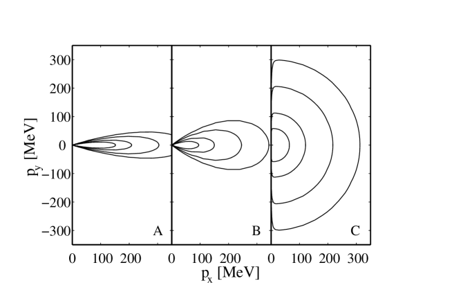
Fig. 5.: The freeze out distribution, $f^{free}(x,\vec{p})$, in the Rest Frame of the freeze out Front (RFF) calculated according to eqs. (42-49). A, B and C correspond to $x=30{\rm fm},\ 80{\rm fm},\ 89.66{\rm fm}$ respectively and $u_{RFG}^{\mu}|_{x=0}=(1,0,0,0)$. We put $N=180\,,N^{\prime}=90\,,m=0\,,n_{0}=1$ and $\sigma={\rm fm}^{2}=10\ {\mu}{\rm barn}$. Contours correspond to $f^{free}=[1,\ 2,\ 4,\ 6]\cdot 10^{-35}(A),10^{-13}(B),10^{-9}(C)\ \frac{fm^{-1}}{\rm MeV^{3}}$. Note that the form of the final freeze out distribution (C) seems to be similar to the cut Jüttner distribution for large $p_{x}$.

Let us define a set of points on the interval $[0$, $L]$ so that:

$$\{x_{i}\},i=1,...,m\,,\quad x_{i}\subset[0,L]\,,\ x_{1}=0,\ x_{m}=L\,.$$ (38)

$$\Delta x_{i}=x_{i+1}-x_{i}\,,\quad 0<{\Delta x_{i}\over L}\ll 1\,.$$ (39)

We assume that $f_{1}(p)=f(0,p)=f^{int}_{1}(p)=f^{int}(0,p)$ is known (i.e. ${\sf n(0)}\,,u^{\mu}(0)$ and $T(0)$ are known). The normalization factor $Z$ can be evaluated as

$$Z(T)\Bigg{|}_{RFF}=\int d^{3}p\ e^{-p^{\mu}u^{int}_{\mu}/T}=4\pi\gamma T^{3}a\left(2K_{1}(a)+K_{0}(a)\right)\stackrel{{\scriptstyle\scriptscriptstyle m=0}}{{\longrightarrow}}8\pi\gamma T^{3}\,.$$ (40)

We have calculated $Z(T)$ in RFF using the same mathematics as in the previous section, and all calculations below will be made in RFF too. The probability $P_{i}(\cos{\theta})\equiv P(x_{i},\cos{\theta})$ is then

$${\cal P}_{i}(\cos\theta)=e^{-N\sigma\frac{\Theta(\cos\theta)}{\cos\theta}+N^{\prime}\frac{\sigma}{\cos\theta}+\frac{\sigma}{\cos\theta}\sum\limits_{j=1}^{i-1}\Delta x_{i}\frac{({\sf n}_{i}+{\sf n}_{i+1})}{2}}\,,\quad{\cal P}_{1}(\cos\theta)\equiv 0\,.$$ (41)

If ${\sf n}(x)$ is a slowly varying function of $x$, we can extrapolate the escape probability by

$$\tilde{\cal P}_{i+1}(\cos\theta)={\cal P}_{i}(\cos\theta)e^{\frac{\sigma}{\cos\theta}\Delta x_{i}{\sf n}_{i}}\,.$$ (42)

Since ${\cal P}_{i}\ll 1$ for almost all values of $x_{i}$, except for the few last nodes, $f^{int}$ is a much more smooth function of $x$ than $f^{free}$, and its extrapolation will be:

$$f^{int}_{i+1}(p)=\left(1-\tilde{\cal P}_{i+1}(\cos\theta)\right)f_{i}(p)\,.$$ (43)

Next we calculate:

$$\tilde{f}_{i+1}(p)=f^{int}_{i+1}(p)+f^{free}_{i}(p)\,,$$ (44)

$$\tilde{{\sf n}}_{i+1}=\int d^{3}p\ \tilde{f}_{i+1}(p)\,,$$ (45)

$${\cal P}_{i+1}(\cos\theta)={\cal P}_{i}(\cos\theta)\ e^{\frac{\sigma}{\cos\theta}\Delta x_{i}\frac{{\sf n}_{i}+\tilde{{\sf n}}_{i+1}}{2}}\,,$$ (46)

$$f^{free}_{i+1}(p)={\cal P}_{i+1}(\cos\theta)\tilde{f}_{i+1}(p)\,,$$ (47)

$$f_{i+1}(p)=f^{int}_{i+1}(p)+f^{free}_{i+1}(p)\,,$$ (48)

$${\sf n}_{i+1}=\int d^{3}pf_{i+1}(p)\,.$$ (49)

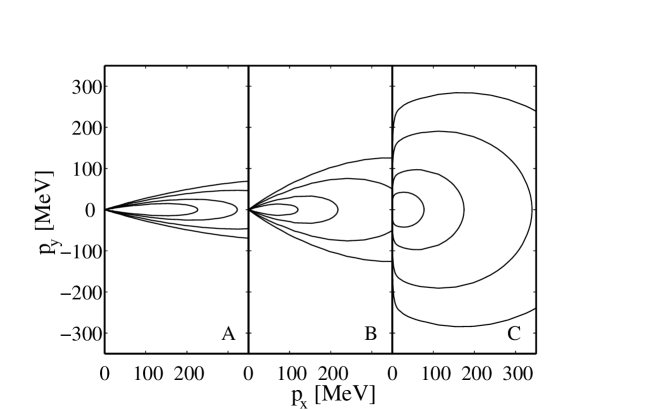
Fig. 6.: The same as Fig. 5, just for $u_{RFG}^{\mu}|_{x=0}=\gamma(1,0.5,0,0)$.

Results received according to such an extrapolation are shown in the Figures 5 - 7. We can see that ${\sf n}(x)$ decreases very sharply and vanishes at point $x=L$, determined from the condition $N=N^{\prime}+\int_{0}^{L}{\sf n}(x)dx$. We can also observe the similarity of Figures 5 with the cut Jüttner distribution. At the same time the initial stages are much more elongated in the $x$ direction in Figures 5 and 6, what may also lead to a large-$p_{t}$ enhancement. This model leads to incomplete freeze out as the one, presented in section 3..   , but such a problem can be cured if rescattering would also be included in the model, as we demonstrated in the previous case.

So far in the calculations described above we did not take into account the conservation laws. Let us check do we break conservation laws or not. According to (43, 47, 48) we have:

$$f_{i+1}(p)=\left(1-\tilde{\cal P}_{i+1}(\cos\theta)\right)f_{i}(p)+{\cal P}_{i+1}(\cos\theta)\left[\left(1-\tilde{\cal P}_{i+1}(\cos\theta)\right)f_{i}(p)+\right.$$

(50)

$$\left.+{\cal P}_{i}\left[\left(1-\tilde{\cal P}_{i}(\cos\theta)\right)f_{i-1}(p)+{\cal P}_{i-1}\left[\left(1-\tilde{\cal P}_{i-1}(\cos\theta)\right)f_{i-2}(p)+...\right]\right]\right]\,.$$

$$f_{i+1}(p)-f_{i}(p)=\left({\cal P}_{i+1}(\cos\theta)-\tilde{\cal P}_{i+1}(\cos\theta)\right)+O\left({\cal P}^{2}\right)\,,$$ (51)

since ${\cal P}_{i}\ll 1$ as well as $\tilde{\cal P}_{i}\ll 1$. Using (42, 46) we get:

$$f_{i+1}(p)-f_{i}(p)={\cal P}_{i}(\cos\theta)e^{\frac{\sigma}{\cos\theta}\Delta x_{i}{{\sf n}_{i}\over 2}}\left(e^{\frac{\sigma}{\cos\theta}\Delta x_{i}{\tilde{{\sf n}}_{i+1}\over 2}}-e^{\frac{\sigma}{\cos\theta}\Delta x_{i}{{\sf n}_{i}\over 2}}\right)f_{i}(p)\,.$$ (52)

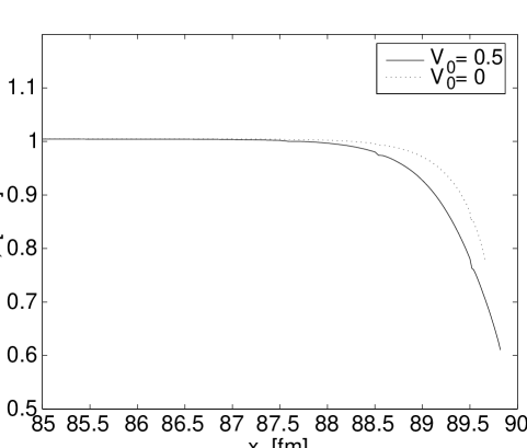
Fig. 7.: Total density ${\sf n}(x)$.We assume $N=180\,,N^{\prime}=90\,,m=0\,,n_{0}=1$ and $\sigma={\rm fm}^{2}=10\ {\mu}{\rm barn}$. We can see ${\sf n}(x)$ is almost the same for $x\subset[0,87]{\rm fm}$, but then it decreases very sharply.

Let us define

$$dF=\frac{d^{3}p}{p^{0}}p^{x}\quad{\rm or}\quad\frac{d^{3}p}{p^{0}}p^{x}p^{0}\quad{\rm or}\quad\frac{d^{3}p}{p^{0}}p^{x}p^{x}\,.$$

Then the conservation laws take the form

$$\int dF\ f_{i}(p)=Const\,,$$ (53)

where $Const=N^{1}(0)\,,\ {\rm or}\ T^{01}(0)\,,\ {\rm or}\ T^{11}(0)$ respectively. Assume that this is true for $f_{i}(p)$, and then let us check $f_{i+1}(p)$.

$${\cal P}_{i}(\cos\theta)=P_{1}(\cos\theta)\ e^{\frac{\sigma{\sf n}_{i}}{\cos\theta}}\,,$$ (54)

where ${\sf n}_{i}=\sum\limits_{j=1}^{i-1}\Delta x_{i}\frac{({\sf n}_{i}+{\sf n}_{i+1})}{2}$, and $P_{1}(\cos\theta)$ is defined by (31). The changes of conserved values at the $i$th step of extrapolation are given by

$$\int dF\left(f_{i+1}(p){-}f_{i}(p)\right)=\int\left(1+\frac{\sigma\Delta x_{i}}{\cos\theta}{{\sf n}_{i}\over 2}\right)\frac{\sigma\Delta x_{i}}{\cos\theta}{(\tilde{{\sf n}}_{i+1}{-}{\sf n}_{i})\over 2}f_{i}(p)P_{1}(\cos\theta)\ e^{\frac{\sigma{\sf n}_{i}}{\cos\theta}}dF\,.$$ (55)

Since $\tilde{{\sf n}}_{i+1}\approx{\sf n}_{i+1}$ with a good accuracy, and ${\cal P}_{i}(\cos\theta)$ has its maximum at $\cos\theta=\pm 1$ (if we put $N^{\prime}={N\over 2}$ we get ${\cal P}_{i}(1)={\cal P}_{i}(-1)$) we have

$$\int dF\left(f_{i+1}(p)-f_{i}(p)\right)\leq P_{1}(1)\ e^{\sigma{\sf n}_{i}}{\sigma\over 2}\left(\frac{d{\sf n}}{dx}\right)_{i}\left(\Delta x_{i}\right)^{2}\cdot Const\,.$$ (56)

Finally,

$$\int dF\left(f_{k}(p)-f_{1}(p)\right)\leq P_{1}(1)\ Const\ {\sigma\over 2}\ \sum\limits_{i=1}^{k-1}e^{\sigma{\sf n}_{i}}\left(\frac{d{\sf n}}{dx}\right)_{i}\left(\Delta x_{i}\right)^{2}\,.$$ (57)

We have seen that $\left(\frac{d{\sf n}}{dx}\right)_{i}\ll 1$ (Fig. 7) and ${\cal P}_{i}(1)\ll 1$ for all $i$, except the last few nodes. So, making $\Delta x_{i}$ small enough, we can keep $dN^{x},\ dT^{0x},\ dT^{xx}$ conserved with the necessary accuracy.

6. Conclusions

In this work we evaluated in a simple kinetic model the freeze out distribution, $f_{free}(x,p)$, for stationary freeze out across a surface with spacelike normal vector, $d\hat{\sigma}^{\mu}d\hat{\sigma}_{\mu}<0$.

The first simple kinetic freeze out model, adopted from [5] (see section 3.. ) reproduces the cut Jüttner distribution as the limiting distribution, $f_{free}$, after complete freeze out at large distances. However, the model at the same time leads to unrealistic consequences, namely that the interacting part of the distribution, $f_{int}$ also survives fully, as the other part of the Jüttner distribution. Thus, having both components at the end in this model, the physical freeze out is actually not realized.

Here we have presented a solution for an improved but still rather approximate kinetic freeze out model which takes rescattering into account (see section 4..5. ). In this model the interacting component is assumed to be instantly re-thermalized taking a spherical Jüttner shape at each time step with changing parameters. The three parameters of the interacting component, $f_{int}$, are obtained in each time step. The density of the interacting component gradually decreases and disappears, the flow velocity also decreases and the energy density decreases also. The temperature, as a consequence of the gradual change in the emission mechanism, gradually decreases at the final stages of the freeze out, when only high energy, forward going particles are taken away from the interacting component.

The arising post freeze out distribution, $f_{free}$ is a superposition of cut Jüttner type of components, from a series of gradually slowing down Jüttner distributions. This leads to a final momentum distribution with a more dominant peak and a forward halo, Fig. 4. In this rough model a large fraction ($\sim 95\%$) of the matter is frozen out by $x=3\lambda$, thus the distribution $f_{free}$ at this distance can be considered as a first estimation of the post freeze out distribution. One should also keep in mind that the model presented here does not have realistic behavior in the limit $x\longrightarrow\infty$, due to its one dimensional character. Nevertheless, this improved model with rescattering enables complete freeze out.

The second model presented here (see section 5..5. ) shows that we can achieve full freeze out in finite length even in oversimplified one dimensional models. Thus, the drawback of the previous model that full freeze out happened exponentially slowly, can be remedied by including more realistic features in the model in a straightforward way.

These studies indicate that more attention should be paid to the final freeze out process, because a more realistic freeze out description may lead to large $p_{t}$ enhancement [24, 25] as the considerations above indicate (Fig. 4). If the heavy ion reaction is basically described by a kinetic model of weakly interacting hadrons, then idealized FO models with an assumed FO hypersurface are on the limits of their applicability, and even then, such models could only be applicable for the heaviest systems.

If, however, QGP is formed in heavy ion reactions, the number of degrees of freedom increases tremendously, and continuum models become more suitable to the problem than dilute gas kinetic or string models with binary interactions. In case of rapid hadronization of QGP and simultaneous freeze out, the idealization of a freeze out hypersurface may be justified, however, an accurate determination of the post freeze out hadron momentum distribution would require a nontrivial dynamical calculation.

Notes

• For the classification scheme see http://www.aip.org/pubservs/pacs.html.

• Assuming that the matter is characterized with 4-velocity $u_{RFG}^{\mu}$, which is normal to the freeze out surface in the three dimensional space, and differs from the Local Rest frame (LR) velocities of $f^{*}_{FO}$, (i.e., $u_{L}^{\mu}$ and $u_{E}^{\mu}$) we introduce here $\tilde{n}(\mu,T)=8\pi T^{3}e^{\mu/T}(2\pi\hbar)^{-3}$,  $a={m\over T}$,  so that $\hat{n}(\mu,T)=\tilde{n}a^{2}K_{2}(a)/2$ is the invariant scalar density of the symmetric massless Jüttner gas, $b=a/\sqrt{1-v^{2}}=a\gamma$,  $v\equiv v_{\sigma}=d\sigma_{0}/d\sigma_{x}=u_{RFG}^{1}|_{RFF}$,  $A=(2+2b+b^{2})e^{-b}$,  and

  $${\cal K}_{n}(z,w)\equiv\frac{2^{n}(n)!}{(2n)!}\ z^{-n}\!\!\int_{w}^{\infty}\!\!\!dx\ (x^{2}-z^{2})^{n-1/2}\ e^{-x}\ ,$$

  i.e. ${\cal K}_{n}(z,z)=K_{n}(z)$. When evaluating the limit we used the relation ${\cal K}_{n}(a,b)\stackrel{{\scriptstyle\scriptstyle a,b=0}}{{\longrightarrow}}K_{n}(a)\stackrel{{\scriptstyle\scriptstyle a=0}}{{\longrightarrow}}(n-1)!\,2^{n-1}a^{-n}$. This baryon current may then be Lorentz transformed into the Eckart Local Rest (ELR) frame of the post FO matter, which moves with $u^{\mu}_{E}=N^{\mu}/(N^{\nu}N_{\nu})^{1/2}=\gamma_{E}(1,v_{E},0,0)|_{RFG}$ in the RFG,  or alternatively into the Rest Frame of the Freeze out front (RFF), where $d\hat{\sigma}_{\mu}=(0,1,0,0)|_{RFF}$ and the velocity of the RFG is $u^{\mu}_{RFG}=\gamma_{\sigma}(1,v,0,0)|_{RFF}$. Then the Eckart flow velocity of the matter represented by the cut Jüttner distribution viewed from the RFF is $u^{\mu}_{E}=\gamma_{c}(1,v_{c},0,0)|_{RFF}$, where $v_{c}=(v+v_{E})/(1+vv_{E})$.

• We are considering fast particles, so that $v_{rel}\sim v$. A formula similar to (21) is also obtained for massless particles.

References

- [1] A.H. Taub, Phys. Rev. 74 (1948) 328.
- [2] L.P. Csernai, Sov. JETP 65 (1987) 216; Zh. Eksp. Theor. Fiz. 92 (1987) 379.
- [3] F. Cooper and G. Frye, Phys. Rev. D 10 (1974) 186.
- [4] K.A. Bugaev, Nucl. Phys. A606 (1996) 559.
- [5] Cs. Anderlik, Zs. Lázár, V.K. Magas, L.P. Csernai, H. Stöcker and W. Greiner, (nucl-th/9808024) Phys. Rev. C 59 (1999) 388.
- [6] Cs. Anderlik, L.P. Csernai, F. Grassi, W. Greiner, Y. Hama, T. Kodama, Zs. Lázár, V.K. Magas and H. Stöcker, (nucl-th/9806004) Phys. Rev. C 59 (1999) in press May 1 issue.
- [7] L.P. Csernai: Introduction to Relativistic Heavy Ion Collisions (Wiley, 1994).
- [8] Yu.M. Sinyukov, Sov. Nucl. Phys. 50 (1989) 228; and Z. Phys. C43 (1989) 401.
- [9] L.V. Bravina, I.N. Mishustin, N.S. Amelin, J.P. Bondorf and L.P. Csernai, Phys. Lett. B354 (1995) 196.
- [10] L.V. Bravina, I.N. Mishustin, J.P. Bondorf and L.P. Csernai, Heavy Ion Phys. 5 (1997) 455.
- [11] H.W. Barz, L.P. Csernai and W. Greiner, Phys. Rev. C26 (1982) 740.
- [12] F. Grassi, Y. Hama and T. Kodama, Phys. Lett. B 355 (1995) 9.
- [13] F. Grassi, Y. Hama and T. Kodama, Z. Phys. C 73 (1996) 153.
- [14] F. Grassi, Y. Hama, T. Kodama and O. Socolowski, Heavy Ion Phys. 5 (1997) 417.
- [15] H. Heiselberg, Heavy Ion Phys. 5 (1997) 435.
- [16] T. Csörgő and L.P. Csernai, Phys. Lett. B333 (1994) 494.
- [17] L.P. Csernai and I.N. Mishustin, Phys. Rev. Lett. 74 (1995) 5005.
- [18] L.P. Csernai and M. Gong, Phys. Rev. D37 (1988) 3231.
- [19] M. Gyulassy and L.P. Csernai, Nucl. Phys. A460 (1986) 723.
- [20] P. Lévai, G. Papp, E. Staubo, A. Holme, D. Strottman and L.P. Csernai, in Proc. of the Int. Workshop on Gross Properties of Nuclei and Nuclear Excitations XVIII, Hirschegg, Austria, Jan. 15-20, 1990 (TH Darmstadt, 1990) p. 90.
- [21] M.I. Gorenstein, Univ. of Frankfurt preprint, UFTP 251/1990.
- [22] J.J. Neumann, B. Lavrenchuk and G. Fai, Heavy Ion Phys. 5 (1997) 27.
- [23] F. Jüttner, Ann. Physik u. Chemie 34 (1911) 865.
- [24] Nu Xu, et al., (NA44), Nucl. Phys. A610 (1997) 175c. (pion spectra in Figs. 4 and 6.)
- [25] P.G. Jones, et al., (NA49), Nucl. Phys. A610 (1997) 188c. ( spectra in Fig. 2.)