SOLAR, SUPERNOVA, AND ATMOSPHERIC NEUTRINOS

In these Canberra summer school lectures we treat a number of topical issues in neutrino astrophysics: the solar neutrino problem, including the physics of the standard solar model, helioseismology, and the possibility that the solution involves new particle physics; atmospheric neutrinos; Dirac and Majorana neutrino masses and their consequences for low-energy weak interactions; red giant evolution as a test of new particle astrophysics; the supernova mechanism; spin-flavor oscillations and oscillations into sterile states, including the effects of density fluctuations; and neutrino-induced and explosive nucleosynthesis.

1 Introduction

The lectures summarized here were originally delivered by the authors at a summer school held in Canberra, Australia, in January, 1998. The written version is a somewhat updated copy of the original, as we have taken this opportunity to include some of the exciting neutrino astrophysics results announced in summer, 1998.

The main theme of these lectures is the interplay between the properties of the neutrinos — their mass, mixing, and charge conjugation properties — and astrophysical phenomena. The first topic is the solar neutrino problem, where we describe the current status of the measurements, the physics of the standard solar model including helioseismology tests, the input nuclear microphysics, and possible solutions. We discuss the MSW mechanism in some detail as well as the potential of SuperKamiokande and SNO to demonstrate that oscillations are occurring.

We then discuss Dirac and Majorana neutrino masses, the seesaw mechanism, and possibilities such as pseudoDirac neutrinos. The associated phenomenology in $\beta$ decay and $\beta\beta$ decay is briefly described.

We discuss a second astrophysical laboratory for neutrino physics, the evolution of red giants. Topics include the nuclear physics of the He flash and the effects of stellar cooling in red giant and horizontal branch stellar evolution. We illustrated how stellar cooling arguments can place powerful constraints on axions and on anomalous properties of the neutrino, such as electric and magnetic dipole moments.

Core-collapse supernovae are the third laboratory. We describe currently favored theories of the explosion mechanism and characterize the spectrum and flavor of the produced neutrinos. We use supernovae and the solar neutrino problem to motivate a discussion of more exotic aspects of the MSW mechanism, including spin-flavor oscillations and the effects of density fluctuations. We also discuss the nucleosynthesis that can arise because of neutrino interactions in the mantle of the star.

We then turn to the explosive nucleosynthesis associated with the supernova shock wave and the neutrino-driven wind off the proto-neutron star surface. We discuss the s- and r-processes, and constraints the latter can place on neutrino oscillations. These constraints prove relevant to certain terrestrial oscillation experiments, such as KARMEN and LSND.

The audience for these lectures consisted of advanced graduate students in nuclear and particle physics: the material is covered at this level and at a depth appropriate to a survey.

2 Solar Neutrinos $\!{}^{{\bf?}}$

More than three decades ago Ray Davis, Jr. and his collaborators $\!{}^{{\bf?}}$ constructed a 0.615 kiloton C₂Cl₄ radiochemical solar neutrino detector in the Homestake Gold Mine, one mile beneath Lead, South Dakota. Within a few years it was apparent that the number of neutrinos detected was considerably below the predictions of the standard solar model, that is, the standard theory of main sequence stellar evolution.

Today the results from the ³⁷Cl detector, which have become quite accurate due to 30 years of careful measurement, have been augmented by results from four other experiments, the SAGE $\!{}^{{\bf?}}$ and GALLEX $\!{}^{{\bf?}}$ gallium experiments and the Kamiokande $\!{}^{{\bf?}}$ and SuperKamiokande $\!{}^{{\bf?}}$ water Cerenkov detectors. It now appears that the combined results are very difficult to explain — some have argued impossible — by any plausible change in the standard solar model (SSM). Thus most believe that the answer to the solar neutrino problem is new particle physics, most likely some effect like solar neutrino oscillations associated with massive neutrinos. With the recent news that SuperKamiokande sees direct evidence for $\nu_{\mu}$ oscillations in the azimuthal dependence of atmospheric $\!{}^{{\bf?}}$ neutrinos, it seems that we may be on the threshold of a major discovery.

The purpose of this first (and longest) lecture is to summarize the solar neutrino problem and to present arguments that it represents new particle physics.

2.1 The Standard Solar Model $\!{}^{{\bf?}}$

Solar models trace the evolution of the Sun over the past 4.6 billion years of main sequence burning, thereby predicting the present-day temperature and composition profiles of the solar core that govern neutrino production. Standard solar models share four basic assumptions:

* The sun evolves in hydrostatic equilibrium, maintaining a local balance between the gravitational force and the pressure gradient. To describe this condition in detail, one must specify the equation of state as a function of temperature, density, and composition.

* Energy is transported by radiation and convection. While the solar envelope is convective, radiative transport dominates in the core region where thermonuclear reactions take place. The opacity depends sensitively on the solar composition, particularly the abundances of heavier elements.

* Thermonuclear reaction chains generate solar energy. The standard model predicts that over 98% of this energy is produced from the pp chain conversion of four protons into ⁴He (see Fig. 1)

$$4p\rightarrow^{4}\mathrm{He}+2e^{+}+2\nu_{e}$$ (1)

with proton burning through the CNO cycle contributing the remaining 2%. The Sun is a large but slow reactor: the core temperature, $T_{c}\sim 1.5\cdot 10^{7}$ K, results in typical center-of-mass energies for reacting particles of $\sim$ 10 keV, much less than the Coulomb barriers inhibiting charged particle nuclear reactions. Thus reaction cross sections are small: in most cases, as laboratory measurements are only possible at higher energies, cross section data must be extrapolated to the solar energies of interest.

* The model is constrained to produce today’s solar radius, mass, and luminosity. An important assumption of the standard model is that the Sun was highly convective, and therefore uniform in composition, when it first entered the main sequence. It is furthermore assumed that the surface abundances of metals (nuclei with A $>$ 5) were undisturbed by the subsequent evolution, and thus provide a record of the initial solar metallicity. The remaining parameter is the initial ⁴He/H ratio, which is adjusted until the model reproduces the present solar luminosity after 4.6 billion years of evolution. The resulting ⁴He/H mass fraction ratio is typically 0.27 $\pm$ 0.01, which can be compared to the big-bang value of 0.23 $\pm$ 0.01. Note that the Sun was formed from previously processed material.

Figure 1: The solar pp chain.

The model that emerges is an evolving Sun. As the core’s chemical composition changes, the opacity and core temperature rise, producing a 44% luminosity increase since the onset of the main sequence. The temperature rise governs the competition between the three cycles of the pp chain: the ppI cycle dominates below about 1.6 $\cdot 10^{7}$ K; the ppII cycle between (1.7-2.3) $\cdot 10^{7}$K; and the ppIII above 2.4 $\cdot 10^{7}$K. The central core temperature of today’s SSM is about 1.55 $\cdot 10^{7}$K.

The competition between the cycles determines the pattern of neutrino fluxes. Thus one consequence of the thermal evolution of our sun is that the ⁸B neutrino flux, the most temperature-dependent component, proves to be of relatively recent origin: the predicted flux increases exponentially with a doubling period of about 0.9 billion years.

A final aspect of SSM evolution is the formation of composition gradients on nuclear burning timescales. Clearly there is a gradual enrichment of the solar core in ⁴He, the ashes of the pp chain. Another element, ³He, is a sort of catalyst for the pp chain, being produced and then consumed, and thus eventually reaching some equilibrium abundance. The timescale for equilibrium to be established as well as the eventual equilibrium abundance are both sharply decreasing functions of temperature, and thus increasing functions of the distance from the center of the core. Thus a steep ³He density gradient is established over time.

The SSM has had some notable successes. From helioseismology the sound speed profile $c(r)$ has been very accurately determined for the outer 90% of the Sun, and is in excellent agreement with the SSM. Such studies verify important predictions of the SSM, such as the depth of the convective zone. However the SSM is not a complete model in that it does not explain all features of solar structure, such as the depletion of surface Li by two orders of magnitude. This is usually attributed to convective processes that operated at some epoch in our sun’s history, dredging Li to a depth where burning takes place.

The principal neutrino-producing reactions of the pp chain and CNO cycle are summarized in Table 1. The first six reactions produce $\beta$ decay neutrino spectra having allowed shapes with endpoints given by E${}_{\nu}^{\rm max}$. Deviations from an allowed spectrum occur for ⁸B neutrinos because the ⁸Be final state is a broad resonance. The last two reactions produce line sources of electron capture neutrinos, with widths $\sim$ 2 keV characteristic of the temperature of the solar core. Measurements of the pp, ⁷Be, and ⁸B neutrino fluxes will determine the relative contributions of the ppI, ppII, and ppIII cycles to solar energy generation. As discussed above, and as later illustrations will show more clearly, this competition is governed in large classes of solar models by a single parameter, the central temperature $T_{c}$. The flux predictions of the 1998 calculations of Bahcall, Basu, and Pinsonneault $\!{}^{{\bf?}}$ (BP98) and of Brun, Turck-Chieze and Morel $\!{}^{{\bf?}}$ are included in Table 1.

Table 1: Solar neutrino sources and the flux predictions of the Bahcall/Pinsonneault (BP98) and Brun/Turck-Chieze/Morel (BTCM98) SSMs in cm^-2s^-1.

Source	E${}_{\nu}^{max}$ (MeV)	BP98	BTCM98
p + p $\rightarrow^{2}$H + e${}^{+}+\nu$	0.42	5.94E10	5.98E10
13N $\rightarrow^{13}$C + e${}^{+}+\nu$	1.20	6.05E8	4.66E8
15O $\rightarrow^{15}$N + e${}^{+}+\nu$	1.73	5.32E8	3.97E8
17F $\rightarrow^{17}$O + e${}^{+}+\nu$	1.74	6.33E6
8B $\rightarrow^{8}$Be + e${}^{+}+\nu$	$\sim$ 15	5.15E6	4.82E6
3He + p $\rightarrow^{4}$He + e${}^{+}+\nu$	18.77	2.10E3
7Be + e${}^{-}\rightarrow^{7}$Li + $\nu$	0.86 (90%)	4.80E9	4.70E9
	0.38 (10%)
p + e- + p $\rightarrow^{2}$H + $\nu$	1.44	1.39E8	1.41E8

2.2 Solar Neutrino Detection $\!{}^{{\bf?}}$

Let us start with a brief reminder about low energy neutrino-nucleus interactions in detectors. Consider the charged current reaction

$$\nu_{e}+(A,Z)\rightarrow e^{-}+(A,Z+1)$$ (2)

Because the momentum transfer to the nucleus is very small for solar neutrinos, it can be neglected in the weak propagator, leading to an effective contact current-current interaction. If we begin with the simplest case of the free neutron decay $n\rightarrow p+e^{-}+\bar{\nu}_{e}$, the corresponding transition amplitude is then

$$S_{fi}={G_{F}\over\sqrt{2}}\cos\theta_{C}\bar{u}(p)\gamma_{\mu}(1-g_{A}\gamma_{5})u(n)\bar{u}(e)\gamma^{\mu}(1-\gamma_{5})u(\nu)$$ (3)

where $G_{F}$ is the weak coupling constant measured in muon decay and $\cos\theta_{c}$ gives the amplitude for the weak interaction to connect the u quark to its first-generation partner, the d quark. The origin of this effective amplitude is the underlying standard model predictions for the elementary quark and lepton currents. The weak interactions at this level are predicted by the standard model to be exactly left handed. Experiment shows that the effective coupling of the W boson to the nucleon is governed by $\gamma_{\mu}(1-g_{A}\gamma_{5})$, as noted above, where $g_{A}\sim 1.26$. The axial coupling is thus shifted from its underlying value by the strong interactions responsible for the binding of the quarks within the nucleon.

If an isolated nucleon were the target, one could proceed to calculate the cross section from the effective nucleon current given above. The extension to nuclear systems traditionally begins with the observation that nucleons in the nucleus are rather non-relativistic, $v/c\sim 0.1$. The amplitude $\bar{u}(p)\gamma^{\mu}(1-g_{A}\gamma_{5})u(n)$ can be expanded in powers of $p/M$. The leading vector and axial operators are readily found to be

$$\gamma_{0} : ~{}~{}~{}1$$

$$\vec{\gamma} : ~{}~{}~{}\vec{p}/M\sim v/c$$

$$\gamma_{0}\gamma_{5} : ~{}~{}~{}\vec{\sigma}\cdot\vec{p}/M\sim v/c$$

$$\vec{\gamma}\gamma_{5} : ~{}~{}~{}\vec{\sigma}$$

Thus it is the time-like part of the vector current and the space-like part of the axial-vector current that survive in the non-relativistic limit.

If such a non-relativistic reduction is done for our single current one obtains

$$S_{fi} \sim \cos\theta_{c}{G_{F}\over\sqrt{2}}(\phi^{\dagger}(p)\phi(n)\bar{u}(e)\gamma^{0}(1-\gamma_{5})u(\nu)$$ (4)

$$-\phi^{\dagger}(p)g_{A}\vec{\sigma}\phi(n)\cdot\bar{u}(e)\vec{\gamma}(1-\gamma_{5})u(\nu))$$

where the $\phi$’s are now two-component Pauli spinors for the nucleons. The above result can be generalized to include $\bar{\nu}_{e}$ reactions by introducing the isospin operators $\tau_{\pm}$ where $\tau_{+}$ $\mid$ n$\rangle$ = $\mid$ p$\rangle$ and $\tau_{-}$$\mid$ p$\rangle$ = $\mid$ n$\rangle$, with all other matrix elements being zero. Thus we can generalize our $n\rightarrow p$ amplitude to $n\leftrightarrow p$ by

$$\phi^{\dagger}(p)\phi(n)\rightarrow\phi^{\dagger}(N)\tau_{\pm}\phi(N)$$

$$\phi^{\dagger}(p)\vec{\sigma}\phi(n)\rightarrow\phi^{\dagger}(N)\vec{\sigma}\tau_{\pm}\phi(N).$$

This result easily generalizes to nuclear decay. Given our comments about exchange currents, the first step is the replacement

$$\tau_{\pm}\rightarrow\sum_{i=1}^{A}\tau_{\pm}(i)$$

$$\sigma\tau_{\pm}\rightarrow\sum_{i=1}^{A}\sigma(i)\tau_{\pm}(i).$$

Plugging $S_{fi}$ into the standard cross section formula (which involves an average over initial and sum over final nuclear spins of the square of the transition amplitude) then yields the allowed nuclear matrix element

$${1\over 2J_{i}+1}\left(|\langle f||\sum_{i=1}^{A}\tau_{\pm}(i)||i\rangle|^{2}+g_{A}^{2}|\langle f||\sum_{i=1}^{A}\sigma(i)\tau_{\pm}(i)||i\rangle|^{2}\right).$$ (5)

Our initial calculation for the nucleon treated that particle as structureless. Implicitly we assumed that the momentum transfer is much smaller than the inverse nucleon size. If we take 10 MeV as a typical solar neutrino momentum transfer, these quantities would be in the ratio 1:20. For a light nucleus, the corresponding result might be 1:10. This long-wavelength approximation in combination with the non-relativistic approximation yields the allowed result, where only Fermi and Gamow-Teller operators survive. These are the spin-independent and spin-dependent operators appearing above.

The Fermi operator is proportional to the isospin raising/lowering operator: in the limit of good isospin, which typically is good to 5% or better in the description of low-lying nuclear states, it can only connect states in the same isospin multiplet, that is, states with a common spin-spatial structure. If the initial state has isospin $(T_{i},M_{Ti})$, this final state has $(T_{i},M_{Ti}\pm 1)$ for $(\nu,e^{-})$ and $(\bar{\nu},e^{+})$ reactions, respectively, and is called the isospin analog state (IAS). In the limit of good isospin the sum rule for this operator in then particularly simple

$$\sum_{f}{1\over 2J_{i}+1}|\langle f||\sum_{i=1}^{A}\tau_{+}(i)||i\rangle|^{2}={1\over 2J_{i}+1}|\langle IAS||\sum_{i=1}^{A}\tau_{+}(i)||i\rangle|^{2}=|N-Z|.$$ (6)

The excitation energy of the IAS relative to the parent ground state can be estimated accurately from the Coulomb energy difference

$$E_{IAS}\sim\left({1.728Z\over 1.12A^{1/3}+0.78}-1.293\right)\mathrm{MeV}.$$ (7)

The angular distribution of the outgoing electron for a pure Fermi $(N,Z)+\nu\rightarrow(N-1,Z+1)+e^{-}$ transition is 1 + $\beta\cos\theta_{\nu e}$, and thus forward peaked. Here $\beta$ is the electron velocity.

The Gamow-Teller (GT) response is more complicated, as the operator can connect the ground state to many states in the final nucleus. In general we do not have a precise probe of the nuclear GT response apart from weak interactions themselves. However a good approximate probe is provided by forward-angle (p,n) scattering off nuclei, a technique that has been developed in particular by experimentalists at the Indiana University Cyclotron Facility$\!{}^{{\bf?}}$. The (p,n) reaction transfers isospin and thus is superficially like $(\nu,e^{-})$. At forward angles (p,n) reactions involve negligible three-momentum transfers to the nucleus. Thus the nucleus should not be radially excited. It thus seems quite plausible that forward-angle (p,n) reactions probe the isospin and spin of the nucleus, the macroscopic quantum numbers, and thus the Fermi and GT responses. For typical transitions, the correspondence between (p,n) and the weak GT operators is believed to be accurate to about 10%. Of course, in a specific transition, much larger discrepancies can arise.

The (p,n) studies demonstrate that the GT strength tends to concentrate in a broad resonance centered at a position $\delta=E_{GT}-E_{IAS}$ relative to the IAS given by

$$\delta\sim\left(7.0-28.9{N-Z\over A}\right)~{}\mathrm{MeV}.$$ (8)

Thus while the peak of the GT resonance is substantially above the IAS for $N\sim Z$ nuclei, it drops with increasing neutron excess. Thus $\delta\sim 0$ for Pb. A typical value for the full width at half maximum $\Gamma$ is $\sim$ 5 MeV.

The approximate Ikeda sum rule constrains the difference in the $(\nu,e^{-})$ and $(\bar{\nu},e^{+})$ strengths

$$\sum_{f}(|M_{GT}^{fi}(\nu,e^{-})|^{2}-|M_{GT}^{fi}(\bar{\nu},e^{+})|^{2})=3(N-Z)$$ (9)

where

$$|M_{GT}^{fi}(\nu,e^{-})|^{2}={1\over 2J_{i}+1}|\langle f||\sum_{i=1}^{A}\sigma(i)\tau_{+}(i)||i\rangle|^{2}.$$ (10)

In many cases of interest in heavy nuclei, the strength in the $(\bar{\nu},e^{+})$ direction is largely blocked. For example, in a naive $2s1d$ shell model description of ³⁷Cl, the p $\rightarrow$ n direction is blocked by the closed neutron shell at N=20. Thus this relation can provide an estimate of the total $\beta^{-}$ strength. Experiment shows that the $\beta^{-}$ strength found in and below the GT resonance does not saturate the Ikeda sum rule, typically accounting for $\sim(60-70)$ % of the total. Measured and shell model predictions of individual GT transition strengths tend to differ systematically by about the same factor. Presumably the missing strength is spread over a broad interval of energies above the GT resonance. This is not unexpected if one keeps in mind that the shell model is an approximate effective theory designed to describe the long wavelength modes of nuclei: such a model should require effective operators, renormalized from their bare values. Phenomenologically, the shell model seems to require $\!{}^{{\bf?}}$ $g_{A}^{eff}\sim$ 1.0 as well as a small spin-tensor term $(\sigma\otimes Y_{2}(\hat{r}))_{J=1}$ of relative strength $\sim$ 0.1.

The angular distribution of GT $(N,Z)+\nu_{e}\rightarrow(N-1,Z+1)+e^{-}$ reactions is $3-\beta\cos\theta_{\nu e}$, corresponding to a gentle peaking in the backward direction.

The above discussion of allowed responses can be repeated for neutral current processes such as $(\nu,\nu^{\prime})$. The analog of the Fermi operator contributes only to elastic processes, where the standard model nuclear weak charge is approximately the neutron number. As this operator does not generate transitions, it is not yet of much interest for solar or supernova neutrino detection, though there are efforts to develop low-threshold detectors (e.g., cryogenic technologies) for recording the modest nuclear recoil energies. The analog of the GT response involves

$$|M_{GT}^{fi}(\nu,\nu^{\prime})|^{2}={1\over 2J_{i}+1}|\langle f||\sum_{i=1}^{A}\sigma(i){\tau_{3}(i)\over 2}||i\rangle|^{2}.$$ (11)

The operator appearing in this expression is familiar from magnetic moments and magnetic transitions, where the large isovector magnetic moment ($\mu_{v}\sim$ 4.706) often leads to it dominating the orbital and isoscalar spin operators.

Finally, there is one purely leptonic reaction of great interest, since it is the reaction exploited by Kamiokande and SuperKamiokande. Electron neutrinos can scatter off electrons via both charged and neutral current reactions. The cross section calculation is straightforward and will not be repeated here. Two features of the result are of importance for our later discussions, however. Because of the neutral current contribution, heavy-flavor $(\nu_{\mu}$ and $\nu_{\tau})$ also scatter off electrons, but with a cross section reduced by about a factor of seven at low energies. Second, for neutrino energies well above the electron rest mass, the scattering is sharply forward peaked. Thus this reaction allows one to exploit the position of the Sun in separating the solar neutrino signal from a large but isotropic background.

As we mentioned earlier, the first experiment performed was one exploiting the reaction

$${}^{37}\mathrm{Cl}(\nu,e^{-})^{37}\mathrm{Ar}.$$

As the threshold for this reaction is 0.814 MeV, the important neutrino sources are the ⁷Be and ⁸B reactions. The ⁷Be neutrinos excite just the GT transition to the ground state, the strength of which is known from the electron capture lifetime of ³⁷Ar. The ⁸B neutrinos can excite all bound states in ³⁷Ar, including the dominant transition to the IAS residing at an excitation of 4.99 MeV. The strength of excite-state GT transitions can be determined from the $\beta$ decay ³⁷Ca$(\beta^{+})^{37}$K, which is the isospin mirror reaction to ³⁷Cl$(\nu,e^{-})^{37}$Ar. The net result is that, for SSM fluxes, 78% of the capture rate should be due to ⁸B neutrinos, and 15% to ⁷Be neutrinos. The measured capture rate $\!{}^{{\bf?}}$ 2.56 $\pm 0.16\pm 0.16$ SNU (1 SNU = 10^-36 capture/atom/sec) is about 1/3 the standard model value.

Similar radiochemical experiments were done by the SAGE and GALLEX collaborations using a different target, ⁷¹Ga. The special properties of this target include its low threshold and an unusually strong transition to the ground state of ⁷¹Ge, leading to a large pp neutrino cross section (see Fig. 2). The experimental capture rates are $66\pm 13\pm 6$ and $76\pm 8$ SNU for the SAGE and GALLEX detectors, respectively. The SSM prediction is about 130 SNU $\!{}^{{\bf?}}$. Most important, since the pp flux is directly constrained by the solar luminosity in all steady-state models, there is a minimum theoretical value for the capture rate of 79 SNU, given standard model weak interaction physics. Note there are substantial uncertainties in the ⁷¹Ga cross section due to ⁷Be neutrino capture to two excited states of unknown strength. These uncertainties were greatly reduced by direct calibrations of both detectors using ⁵¹Cr neutrino sources.

Figure 2: Level scheme for ⁷¹Ge showing the excited states that contribute to absorption of pp, ⁷Be, ⁵¹Cr, and ⁸B neutrinos.

The remaining experiments, Kamiokande II/III and SuperKamiokande, exploited water Cerenkov detectors to view solar neutrinos on an event-by-event basis. Solar neutrinos scatter off electrons, with the recoiling electrons producing the Cerenkov radiation that is then recorded in surrounding photo-tubes. Thresholds are determined by background rates; SuperKamiokande is currently operating with a trigger at approximately 6 MeV. The initial experiment, Kamiokande II/III, found a flux of ⁸B neutrinos of (2.91 $\pm 0.24\pm 0.35)\cdot 10^{6}$/cm²s after about a decade of measurement. Its much larger successor SuperKamiokande, with a 22.5 kiloton fiducial volume, yielded the result $(2.44\pm 0.05^{+0.09}_{-0.07})\cdot 10^{6}$/cm²s after the first 504 days of measurements$\!{}^{{\bf?}}$. This is about half of the SSM flux. This result continues to improve in accuracy.

2.3 Uncertainties in Standard Solar Model Parameters

The pattern of solar neutrino fluxes that has emerged from these experiments is

$$\phi(pp) \sim 0.9\,\phi^{\rm{SSM}}(pp)$$

$$\phi(^{7}{\rm{Be}}) \sim 0$$

$$\phi(^{8}{\rm B}) \sim 0.43\,\phi^{\rm{SSM}}(^{8}{\rm B}).$$ (12)

A reduced ⁸B neutrino flux can be produced by lowering the central temperature of the sun somewhat, as $\phi(^{8}$B)$\sim T_{c}^{18}$. However, such an adjustment, either by varying the parameters of the SSM or by adopting some nonstandard physics, tends to push the $\phi(^{7}$Be)/$\phi(^{8}$B) ratio to higher values rather than the low one of eq. (12),

$${\phi(^{7}{\rm{Be}})\over\phi(^{8}{\rm B})}\sim T_{c}^{-10}.$$ (13)

Thus the observations seem difficult to reconcile with plausible solar model variations: one observable, $\phi(^{8}$B), requires a cooler core while a second, the ratio $\phi(^{7}$Be)/$\phi(^{8}$B), requires a hotter one.

An initial question is whether this problem remains significant when one takes into account known uncertainties in the parameters of the SSM. While a detailed summary of the SSM uncertainties would take us well beyond the limits of these lectures, a qualitative discussion of pp chain nuclear uncertainties is appropriate. This nuclear microphysics has been the focus of a great deal of experimental work. The pp chain involves a series of non-resonant charged-particle reactions occurring at center-of-mass energies that are well below the height of the inhibiting Coulomb barriers. As the resulting small cross sections generally preclude laboratory measurements at the relevant energies, one must extrapolate higher energy measurements to threshold to obtain solar cross sections. This extrapolation is often discussed in terms of the astrophysical S-factor

$$\sigma(E)={S(E)\over E}\exp(-2\pi\eta)$$ (14)

where $\eta={Z_{1}Z_{2}\alpha\over\beta}$, with $\alpha$ the fine structure constant and $\beta=v/c$ the relative velocity of the colliding particles. This parameterization removes the gross Coulomb effects associated with the s-wave interactions of charged, point-like particles. The remaining energy dependence of S(E) is gentle and can be expressed as a low-order polynomial in E. Usually the variation of S(E) with E is taken from a direct reaction model and then used to extrapolate higher energy measurements to threshold. The model accounts for finite nuclear size effects, strong interaction effects, contributions from other partial waves, etc. As laboratory measurements are made with atomic nuclei while conditions in the solar core guarantee the complete ionization of light nuclei, additional corrections must be made to account for the different electronic screening environments.

Recently a large working group met at a workshop sponsored by the Institute for Nuclear Theory, University of Washington, to review past work on the nuclear reactions of the pp chain and CNO cycle, to recommend best values and appropriate errors, and to identify specific issues in experiment and theory where additional work is needed. The results are published in Reviews of Modern Physics$\!{}^{{\bf?}}$. We will not attempt a summary here, but will give one or two highlights.

The most significant recommend change involves the reaction ⁷Be(p, $\gamma)\,^{8}$B, where the standard S₁₇(0)$\sim$ 22.4 eVb is that given $\!{}^{{\bf?}}$ by Johnson et al. Measurements of S₁₇(E) are complicated by the need to use radioactive targets and thus to determine the areal density of the ⁷Be target nuclei. Two techniques have been employed, measuring the rate of 478 keV photons from ⁷Be decay or counting the daughter ⁷Li nuclei via the reaction ⁷Li (d,p)⁸Li. The low-energy data sets for S₁₇(E) disagree by 25%. This is a systematic normalization problem as each data set is consistent with theory in its dependence on E. The energy dependence below $\sim$ 500 keV is believed to be quite simple as it is determined by the asymptotic nuclear wave function.

The Seattle working group on S₁₇(E) found that only one low-energy data set, that of Filippone et al. $\!{}^{{\bf?}}$, was described in the published literature in sufficient detail to be evaluated. The target activity in that experiment had been measured by both 478 keV gamma rays and by the (d,p) reaction, with consistent results. The resulting recommended value was thus based on this measurement, yielding

$$S_{17}(0)=19^{+4}_{-2}\mathrm{eV~{}b},~{}~{}1\sigma.$$ (15)

A recent measurement$\!{}^{{\bf?}}$ is consistent with this value.

The ³He($\alpha,\gamma)^{7}$Be reaction has been measured by two techniques, by counting the capture $\gamma$ rays and by detecting the resulting ⁷Be activity. While the two techniques have been used by several groups and have yielded separately consistent results, the capture $\gamma$ ray value S₁₇(0) = 0.507 $\pm$ 0.016 keV b is not in good agreement with the ⁷Be activity value 0.572 $\pm$ 0.026 keV-b. The Seattle working group concluded that the evidence for a systematic discrepancy of unknown origin was reasonably strong and recommended that standard procedures be used in assigning a suitably expanded error. The recommended value S₃₄ (0) is 0.53 $\pm$ 0.05.

These and other recommended values were recently incorporated into the BP98 and BTCM98 solar model calculations. While the workshop’s recommended values involve no qualitative changes, there is some broadening of error bars. The downward shift in S₁₇(0) leads to a lower ⁸B flux. The workshop’s Reviews of Modern Physics article summarizes a substantial amount of work on topics not discussed here: screening effects, weak radiative corrections to and exchange current effects on p+p, the atomic physics of ⁷Be + e^-, etc. Much of this discussion was useful in evaluating possible uncertainties in solar microphysics, and in identifying opportunities for reducing these uncertainties.

Are uncertainties in the parameters of the SSM a significant source of uncertainty? The S-factors discussed above comprise one set of parameters, but there are others: the solar lifetime, the opacities, the solar luminosity, etc. In order to answer this question while also taking into account correlations among the fluxes when input parameters are varied, first Bahcall and Ulrich $\!{}^{{\bf?}}$ and later Bahcall and Haxton $\!{}^{{\bf?}}$ constructed 1000 SSMs by randomly varying five input parameters, the primordial heavy-element-to-hydrogen ratio Z/X and S(0) for the p-p, ³He-³He, ³He-⁴He, and p-⁷Be reactions, assuming for each parameter a normal distribution with the mean and standard deviation. (These were the parameters assigned the largest uncertainties.) Smaller uncertainties from radiative opacities, the solar luminosity, and the solar age were folded into the results of the model calculations perturbatively.

The resulting pattern of ⁷Be and ⁸B flux predictions is shown in Fig. 3. The elongated error ellipses indicate that the fluxes are strongly correlated. Those variations producing $\phi(^{8}$B) below 0.8$\phi^{\rm{SSM}}(^{8}$B) tend to produce a reduced $\phi(^{7}$Be), but the reduction is always less than 0.8. Thus a greatly reduced $\phi(^{7}$Be) cannot be achieved within the uncertainties assigned to parameters in the SSM.

Figure 3: SSM ⁷Be and ${}^{8}B$ flux predictions. The dots represent the results of SSM calculations where the input parameters were varied according to their assigned uncertainties, as described in the text. The 90% and 99% confidence level error ellipses are shown.

A similar exploration, but including parameter variations very far from their preferred values, was carried out by Castellani et al. $\!{}^{{\bf?}}$, who displayed their results as a function of the resulting core temperature $T_{c}$. The pattern that emerges is striking (see Fig. 4): parameter variations producing the same value of $T_{c}$ produce remarkably similar fluxes. Thus $T_{c}$ provides an excellent one-parameter description of standard model perturbations. Figure 4 also illustrates the difficulty of producing a low ratio of $\phi(^{7}$Be)/$\phi(^{8}$B) when $T_{c}$ is reduced.

The 1000-solar-model variations were made under the constraint of reproducing the solar luminosity. Those variations show a similar strong correlation with $T_{c}$

$$\phi(pp)\propto T_{c}^{-1.2}~{}~{}~{}~{}~{}~{}~{}\phi(^{7}{\rm{Be}})\propto T_{c}^{8}~{}~{}~{}~{}~{}~{}~{}\phi(^{8}{\rm B})\propto T_{c}^{18}.$$ (16)

Figures 3 and 4 offer a strong argument that reasonable variations in the parameters of the SSM, or nonstandard changes in quantities like the metallicity, opacities, or solar age, cannot produce the pattern of fluxes deduced from experiment (eq. (12)). This would seem to limit possible solutions to errors either in the underlying physics of the SSM or in our understanding of neutrino properties.

Figure 4: The responses of the pp, ⁷Be, and ⁸B neutrino fluxes to the indicated variations in solar model input parameters, displayed as a function of the resulting central temperature $T_{c}$. From Castellani et al.

2.4 Nonstandard Solar Models

Nonstandard solar models include both variations of SSM parameters far outside the ranges that are generally believed to be reasonable (some examples of which are given in Figure 4), and changes in the underlying physics of the model. The solar neutrino problem has been a major stimulus to models: in fact, most suggestions were motivated by the hope of producing a cooler Sun ($T_{c}\sim 0.95T_{c}$) that would avoid conflict with the results of the ³⁷Cl experiment. The suggestions included models with low heavy element abundances (“low Z” models), in which one abandons the SSM assumption that the initial heavy element abundances are those we measure today at the Sun’s surface; periodically mixed solar cores; models where hydrogen is continually mixed into the core by turbulent diffusion or by convective mixing; and models where the solar core is partially supported by a strong central magnetic field or by its rapid rotation, thereby relaxing the SSM assumption that hydrostatic equilibrium is achieved only through the gas pressure gradient. A larger list is given by Bahcall and Davis $\!{}^{{\bf?}}$. To illustrate the kinds of consequences such models have, two of these suggestions are discussed in more detail below.

In low-Z models one postulates a reduction in the core metallicity from Z $\sim$ 0.02 to Z $\sim$ 0.002. This lowers the core opacity (primarily because metals are very important to free-bound electron transitions), thus reducing $T_{c}$ and weakening the ppII and ppIII cycles. The attractiveness of low-Z models is due in part to the existence of additional mechanisms for adding heavier elements to the Sun’s surface. These include the infall of comets and other debris, as well as the accumulation of dust as the Sun passes through interstellar clouds. However, the increased radiative energy transport in low-Z models leads to a thin convective envelope, in contradiction to interpretations of the 5-minute solar surface oscillations. A low He mass fraction also results. As diffusion of material from a thin convective envelope into the interior would deplete heavy elements at the surface, investigators have also questioned whether present abundances could have accumulated in low-Z models. Finally, the general consistency of solar heavy element abundances with those observed in other main sequence stars makes the model appear contrived.

Models in which the solar core ($\sim$ 0.2 M_⊙) is intermittently mixed break the standard model assumption of a steady-state Sun: for a period of several million years (the thermal relaxation time for the core) following mixing, the usual relationship between the observed surface luminosity and rate of energy (and neutrino) production is altered as the Sun burns out of equilibrium. Calculations show that both the luminosity and the ⁸B neutrino flux are suppressed while the Sun relaxes back to the steady state. Such models have been considered seriously because of instabilities associated with large gradients in the ³He abundance, which in equilibrium varies as $\sim T^{-6}$, where $T$ is the local temperature. The resulting steep profile is unstable under finite amplitude displacements of a volume to smaller r: the energy released by the increased ³He burning at higher T can exceed the energy in the perturbation. For a discussion of the plausibility of such a trigger for core mixing, one can see the original work of Dilke and Gough $\!{}^{{\bf?}}$ as well as a more recent critique by Merryfield $\!{}^{{\bf?}}$. The possibility that continuous mixing on time scales of ³He mixing could produce a flux pattern close to that observed (e.g., a suppression in both the ⁸B neutrino flux and the ⁷Be/⁸B flux ratio) was recently discussed by Cumming and Haxton $\!{}^{{\bf?}}$.

This discussion of two of the more seriously explored nonstandard model possibilities illustrates how changes motivated by the solar neutrino problem often produce other, unwanted consequences. In particular, many experts feel that the good SSM agreement with helioseismology is likely to be destroyed by changes such as those discussed above.

Figure 5 is an illustration by Hata et al. $\!{}^{{\bf?}}$ of the flux predictions of several nonstandard models, including a low-Z model consistent with the ³⁷Cl results. As in the Castellani et al. exploration, the results cluster along a track that defines the naive $T_{c}$ dependence of the $\phi(^{7}$Be)/$\phi(^{8}$B) ratio, well separated from the experimental contours.

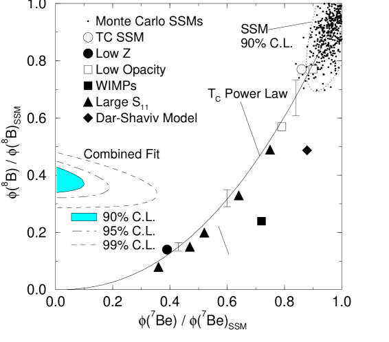
Figure 5: The fluxes allowed by the combined results of the various solar neutrino experiments compared to the results of SSM variations and various nonstandard solar models. The solid line in the naive $T_{c}$ power law discussed in the text. From Hata et al.

There is now a popular argument that no such nonstandard model can solve the solar neutrino problem: if one assumes undistorted neutrino spectra, no combination of pp, ⁷Be, and ⁸B neutrino fluxes fits the experimental results well $\!{}^{{\bf?}}$. In fact, in an unconstrained fit, the required ⁷Be flux is unphysical, negative by almost 3$\sigma$. Thus, barring some unfortunate experimental error, it appears we are forced to look elsewhere for a solution.

If experimental error, SSM parameter uncertainties, and nonstandard solar physics are ruled out as potential solutions, new particle physics is left as the leading possibility. Suggested particle physics solutions of the solar neutrino problem include neutrino oscillations, neutrino decay, neutrino magnetic moments, and weakly interacting massive particles. Among these, the Mikheyev-Smirnov-Wolfenstein effect — neutrino oscillations enhanced by matter interactions — is widely regarded as the most plausible.

2.5 Helioseismology

Earlier it was mentioned that measurements of the sound velocity within the Sun, deduced from observations of surface oscillations, provide a powerful check on the SSM. In this section the basic physics of helioseismology is reviewed.

A static, stable star at spherically-symmetric equilibrium can be characterized with pressure $p(r)$, mass density $\rho(r)$, the gravitational potential $\phi(r)$, the rate of nuclear energy generation $\epsilon(r)$, temperature $T(r)$, the energy flux F and the entropy $s$. Introducing the adiabatic indices

$$\Gamma_{1}=\left({\partial\log p\over\partial\log\rho}\right)_{s},$$ (17)

$$\Gamma_{3}-1=\left({\partial\log T\over\partial\log\rho}\right)_{s},$$ (18)

and the total derivative

$${D\over Dt}={\partial\over\partial t}+{\bf v}\cdot\nabla$$ (19)

one can write down the equation of motion

$$\rho{D{\bf v}\over Dt}=-\nabla p-\rho\nabla\phi,$$ (20)

the equation of continuity

$${D\rho\over Dt}+\rho\nabla\cdot{\bf v}=0,$$ (21)

Poisson’s equation for gravitational attraction

$$\nabla^{2}\phi=4\pi G\rho,$$ (22)

and an equation describing energy conservation

$${1\over p}{Dp\over Dt}-\Gamma_{1}{1\over\rho}{D\rho\over Dt}={{\Gamma_{3}-1}\over p}(\rho\epsilon-\nabla\cdot{\bf F}).$$ (23)

These equations describe a static star. To do stellar seismology one introduces Eulerian (i.e. at a given point) perturbations on the physical quantities, e.g.

$$\rho({\bf r},t)=\rho_{0}({\bf r})+\rho^{\prime}({\bf r},t)$$ (24)

where $\rho_{0}$ denotes the equilibrium value and the displacement is calculated from the velocity amplitude

$${\bf v}={\partial\over\partial t}(\delta{\bf r}).$$ (25)

Inserting expressions like Eq. (24) in the above equations and subtracting the equilibrium equations one obtains equations that describe the perturbations. From the conservation of momentum one gets

$$\rho{\partial^{2}\delta{\bf r}\over\partial t^{2}}=-\nabla p^{\prime}+{\rho^{\prime}\over\rho}\nabla p-\rho\nabla\phi^{\prime}.$$ (26)

The equation of continuity gives

$$\rho^{\prime}+\nabla\cdot(\rho\delta{\bf r})=0.$$ (27)

Poisson’s equation becomes

$$\nabla^{2}\phi^{\prime}=4\pi G\rho^{\prime},$$ (28)

and the energy equation yields

$${\rho^{\prime}\over\rho}+{1\over\rho}\delta{\bf r}\cdot\nabla\rho={1\over\Gamma_{1}}\left({p^{\prime}\over p}+{1\over p}\delta{\bf r}\cdot\nabla p\right).$$ (29)

In these equations for convenience we dropped the subscript zero in writing down the equilibrium values. To obtain the normal modes of a star we assume a time dependence of $\exp(-i\omega t)$ for the perturbations:

$$\rho^{\prime}({\bf r},t)\sim\rho^{\prime}(r)Y_{\ell m}(\theta,\phi)\exp(-i\omega t).$$ (30)

Using Eq. (30) and introducing the auxiliary quantity

$$\Psi(r)=c^{2}\rho^{1/2}\nabla\cdot\delta{\bf r},$$ (31)

where $c$ is the adiabatic sound speed

$$c^{2}={\Gamma_{1}p\over\rho},$$ (32)

Eqs. (26) through (29) can be written in a compact form

$${d^{2}\Psi\over dr^{2}}+{1\over c^{2}}\left[\omega^{2}-\omega^{2}_{\rm co}-{\ell(\ell+1)c^{2}\over r^{2}}\left(1-{N^{2}\over\omega^{2}}\right)\right]\Psi\simeq 0.$$ (33)

In Eq. (33) we used the buoyancy frequency:

$$N^{2}={Gm_{0}(r)\over r}\left({1\over\Gamma_{1}}{d\log p\over dr}-{d\log\rho\over dr}\right),$$ (34)

and the acoustical cut-off frequency

$$\omega^{2}_{\rm co}={c^{2}\over 4H^{2}}\left(1-2{dH\over dr}\right),$$ (35)

where the density scale height is

$$H=-(d\log\rho/dr)^{-1}.$$ (36)

One observes that oscillation frequencies are determined by the sound speed profile. The sound speed profile calculated using the Bahcall-Pinsonneault 1998 SSM is shown in Figure 6.

Figure 6: Sound speed profile in the Sun. From Bahcall and Pinsonneault.

Eq. (33) resembles the Schroedinger equation in quantum mechanics. For the present Sun the buoyancy frequency is approximately constant in the radiative zone except very near the core, but vanishes in the convective zone. The acoustical cut-off frequency is a monotonically decreasing function of the distance from the center of the Sun. Inserting this “potential” to the “Schroedinger equation”, Eq. (33), one observes that for $N^{2}/\omega^{2}\ll 1$ the amplitude of the oscillations die out in the radiative zone (“classically forbidden”) of the Sun. The resulting oscillations are confined to the convective (outer) zone of the Sun and called p-modes (for pressure). For ${\ell(\ell+1)c^{2}\over r^{2}\omega^{2}}\gg 1$ the situation is reversed. The “classically allowed” region is the core of the Sun and the amplitudes die out in the convective zone. These oscillations are called g-modes (for gravity). Note that g-mode oscillation amplitudes vanish at the solar surface, hence it is very difficult to directly observe g-modes. On the other hand p-mode oscillations are readily measurable by observing the solar surface. Eq. (33) indicates that p-mode oscillations with different $\ell$ values penetrate to different depths, the observed frequencies $\omega_{\ell}$ are determined by conditions at different parts of the Sun.

It is possible to gain insight to the properties of solar oscillations by regarding the equations outlined above as an eigenvalue problem in a linear Hilbert space. Hence it is possible to directly relate perturbations in the sound speed to the perturbations in $\omega_{\ell}$. One starts with the sound speed profile and oscillation frequencies calculated in a reference solar model. These quantities are taken as the unperturbed quantities. Then using standard Raleigh-Schroedinger perturbation theory one relates the difference between observed and calculated frequencies to the deviation of the sound speed from the model prediction. A very readable introduction the the theoretical aspects of helioseismology is available on the world wide web $\!{}^{{\bf?}}$. There is very good agreement between calculated and observed sound speeds in the Sun. Figure 7 shows the fractional difference between the predicted and observed sound speed profiles $\!{}^{{\bf?}}$. Sound speed profiles deduced from helioseismology provides an important constraint on solar models.

Figure 7: Fractional difference between the predicted and observed sound speed profiles. From Bahcall, Basu, and Pinsonneault.

2.6 Neutrino Oscillations

One odd feature of particle physics is that neutrinos, which are not required by any symmetry to be massless, nevertheless must be much lighter than any of the other known fermions. For instance, the current limit on the $\overline{\nu}_{e}$ mass is $\mathrel{\hbox to0.0pt{\lower 4.0pt\hbox{\hskip 1.0pt$\sim$}\hss}\raise 1.0pt\hbox{$<$}}$ 5 eV. The standard model requires neutrinos to be massless, but the reasons are not fundamental. Dirac mass terms $m_{D}$, analogous to the mass terms for other fermions, cannot be constructed because the model contains no right-handed neutrino fields. Neutrinos can also have Majorana mass terms

$$\overline{\nu^{c}_{L}}m_{L}\nu_{L}~{}~{}~{}\mathrm{and}~{}~{}~{}\overline{\nu^{c}_{R}}m_{R}\nu_{R}$$ (37)

where the subscripts $L$ and $R$ denote left- and right-handed projections of the neutrino field $\nu$, and the superscript $c$ denotes charge conjugation. The first term above is constructed from left-handed fields, but can only arise as a nonrenormalizable effective interaction when one is constrained to generate $m_{L}$ with the doublet scalar field of the standard model. The second term is absent from the standard model because there are no right-handed neutrino fields.

None of these standard model arguments carries over to the more general, unified theories that theorists believe will supplant the standard model. In the enlarged multiplets of extended models it is natural to characterize the fermions of a single family, e.g., $\nu_{e}$, e, u, d, by the same mass scale $m_{D}$. Small neutrino masses are then frequently explained as a result of the Majorana neutrino masses. In the seesaw mechanism$\!{}^{{\bf?}}$,

$$M_{\nu}\sim\left(\begin{array}[]{cc}0&m_{D}\\ m^{T}_{D}&m_{R}\end{array}\right).$$ (38)

Diagonalization of the mass matrix produces one light neutrino, $m_{\mathrm{light}}\sim{m_{D}^{2}\over m_{R}}$, and one unobservably heavy, $m_{\mathrm{heavy}}\sim m_{R}$. The factor ($m_{D}$/$m_{R}$) is the needed small parameter that accounts for the distinct scale of neutrino masses. The masses for the $\nu_{e},\nu_{\mu}$, and $\nu_{\tau}$ are then related to the squares of the corresponding quark masses $m_{u}$, $m_{c}$, and $m_{t}$. Taking $m_{R}\sim 10^{16}$ GeV, a typical grand unification scale for models built on groups like SO(10), the seesaw mechanism gives the crude relation

$$m_{\nu_{e}}:m_{\nu_{\mu}}:m_{\nu_{\tau}}\leftrightarrow 2\cdot 10^{-12}:2\cdot 10^{-7}:3\cdot 10^{-3}\mathrm{eV}.$$ (39)

The fact that solar neutrino experiments can probe small neutrino masses, and thus provide insight into possible new mass scales $m_{R}$ that are far beyond the reach of direct accelerator measurements, has been an important theme of the field.

One of the most interesting possibilities for solving the solar neutrino problem has to do with neutrino masses. For simplicity we will discuss just two neutrinos. If a neutrino has a mass $m$, we mean that as it propagates through free space, its energy and momentum are related in the usual way for this mass. Thus if we have two neutrinos, we can label those neutrinos according to the eigenstates of the free Hamiltonian, that is, as mass eigenstates.

But neutrinos are produced by the weak interaction. In this case, we have another set of eigenstates, the flavor eigenstates. We can define a $\nu_{e}$ as the neutrino that accompanies the positron in $\beta$ decay. Likewise we label by $\nu_{\mu}$ the neutrino produced in muon decay.

Now the question: are the eigenstates of the free Hamiltonian and of the weak interaction Hamiltonian identical? Most likely the answer is no: we know this is the case with the quarks, since the different families (the analog of the mass eigenstates) do interact through the weak interaction. That is, the up quark decays not only to the down quark, but also occasionally to the strange quark. (This is why we had a $\cos\theta_{c}$ in our weak interaction amplitude: the amplitude for $u\rightarrow s$ is proportional to $\sin\theta_{c}$.) Thus we suspect that the weak interaction and mass eigenstates, while spanning the same two-neutrino space, are not coincident: the mass eigenstates $|\nu_{1}\rangle$ and $|\nu_{2}\rangle$ (with masses $m_{1}$ and $m_{2}$) are related to the weak interaction eigenstates by

$$|\nu_{e}\rangle = \cos\theta_{v}|\nu_{1}\rangle+\sin\theta_{v}|\nu_{2}\rangle$$

$$|\nu_{\mu}\rangle = -\sin\theta_{v}|\nu_{1}\rangle+\cos\theta_{v}|\nu_{2}\rangle$$ (40)

where $\theta_{v}$ is the (vacuum) mixing angle.

An immediate consequence is that a state produced as a $|\nu_{e}\rangle$ or a $|\nu_{\mu}\rangle$ at some time $t$ — for example, a neutrino produced in $\beta$ decay — does not remain a pure flavor eigenstate as it propagates away from the source. This is because the different mass eigenstates comprising the neutrino will accumulate different phases as they propagate downstream, a phenomenon known as vacuum oscillations (vacuum because the experiment is done in free space). To see the effect, suppose we produce a neutrino in some $\beta$ decay where we measure the momentum of the initial nucleus, final nucleus, and positron. Thus the outgoing neutrino is a momentum eigenstate $\!{}^{{\bf?}}$. At time $t$=0

$$|\nu(t=0)\rangle=|\nu_{e}\rangle=\cos\theta_{v}|\nu_{1}\rangle+\sin\theta_{v}|\nu_{2}\rangle.$$ (41)

Each eigenstate subsequently propagates with a phase

$$e^{i(\vec{k}\cdot\vec{x}-\omega t)}=e^{i(\vec{k}\cdot\vec{x}-\sqrt{m_{i}^{2}+k^{2}}t)}.$$ (42)

But if the neutrino mass is small compared to the neutrino momentum/energy, one can write

$$\sqrt{m_{i}^{2}+k^{2}}\sim k(1+{m_{i}^{2}\over 2k^{2}}).$$ (43)

Thus we conclude

$$|\nu(t)\rangle = e^{i(\vec{k}\cdot\vec{x}-kt-(m_{1}^{2}+m_{2}^{2})t/4k)}$$ (44)

$$\times[\cos\theta_{v}|\nu_{1}\rangle e^{i\delta m^{2}t/4k}+\sin\theta_{v}|\nu_{2}\rangle e^{-i\delta m^{2}t/4k}].$$

We see there is a common average phase (which has no physical consequence) as well as a beat phase that depends on

$$\delta m^{2}=m_{2}^{2}-m_{1}^{2}.$$ (45)

Now it is a simple matter to calculate the probability that our neutrino state remains a $|\nu_{e}\rangle$ at time t

$$P_{\nu_{e}}(t) = |\langle\nu_{e}|\nu(t)\rangle|^{2}$$ (46)

$$= 1-\sin^{2}2\theta_{v}\sin^{2}\left({\delta m^{2}t\over 4k}\right)\rightarrow 1-{1\over 2}\sin^{2}2\theta_{v}$$

where the limit on the right is appropriate for large $t$. Now $E\sim k$, where E is the neutrino energy, by our assumption that the neutrino masses are small compared to $k$. Thus we can reinsert the units above to write the probability in terms of the distance $x$ of the neutrino from its source,

$$P_{\nu}(x)=1-\sin^{2}2\theta_{v}\sin^{2}\left({\delta m^{2}c^{4}x\over 4\hbar cE}\right).$$ (47)

(When one properly describes the neutrino state as a wave packet, the large-distance behavior follows from the eventual separation of the mass eigenstates.) If the the oscillation length

$$L_{o}={4\pi\hbar cE\over\delta m^{2}c^{4}}$$ (48)

is comparable to or shorter than one astronomical unit, a reduction in the solar $\nu_{e}$ flux would be expected in terrestrial neutrino oscillations.

The suggestion that the solar neutrino problem could be explained by neutrino oscillations was first made by Pontecorvo in 1958, who pointed out the analogy with $K_{0}\leftrightarrow\bar{K}_{0}$ oscillations. From the point of view of particle physics, the sun is a marvelous neutrino source. The neutrinos travel a long distance and have low energies ($\sim$ 1 MeV), implying a sensitivity down to

$$\delta m^{2}\mathrel{\hbox to0.0pt{\lower 4.0pt\hbox{\hskip 1.0pt$\sim$}\hss}\raise 1.0pt\hbox{$>$}}10^{-12}eV^{2}.$$ (49)

In the seesaw mechanism, $\delta m^{2}\sim m^{2}_{2}$, so neutrino masses as low as $m_{2}\sim 10^{-6}$ eV could be probed. In contrast, terrestrial oscillation experiments with accelerator or reactor neutrinos are typically limited to $\delta m^{2}\mathrel{\hbox to0.0pt{\lower 4.0pt\hbox{\hskip 1.0pt$\sim$}\hss}\raise 1.0pt\hbox{$>$}}0.1$ eV².

From the expressions above one expects vacuum oscillations to affect all neutrino species equally, if the oscillation length is small compared to an astronomical unit. This is somewhat in conflict with the solar neutrino data, as we have argued that the ⁷Be neutrino flux is quite suppressed. Furthermore, there is a weak theoretical prejudice that $\theta_{v}$ should be small, like the Cabibbo angle. The first objection, however, can be circumvented in the case of “just so” oscillations where the oscillation length is comparable to one astronomical unit. In this case the oscillation probability becomes sharply energy dependent, and one can choose $\delta m^{2}$ to preferentially suppress one component (e.g., the monochromatic ⁷Be neutrinos). This scenario has been explored by several groups and remains an interesting possibility. However, the requirement of large mixing angles remains.

Below we will see that stars allow us to “get around” this problem with small mixing angles. In preparation for this, we first present the results above in a slightly more general way. The analog of Eq. (44) for an initial muon neutrino ($|\nu(t=0)\rangle=|\nu_{\mu}\rangle$) is

$$|\nu(t)\rangle = e^{i(\vec{k}\cdot\vec{x}-kt-(m_{1}^{2}+m_{2}^{2})t/4k)}$$ (50)

$$\times[-\sin\theta_{v}|\nu_{1}\rangle e^{i\delta m^{2}t/4k}+\cos\theta_{v}|\nu_{2}\rangle e^{-i\delta m^{2}t/4k}]$$

Now if we compare Eqs. (44) and (50) we see that they are special cases of a more general problem. Suppose we write our initial neutrino wave function as

$$|\nu(t=0)\rangle=a_{e}(t=0)|\nu_{e}\rangle+a_{\mu}(t=0)|\nu_{\mu}\rangle.$$ (51)

Then Eqs. (44) and (50) tell us that the subsequent propagation is described by changes in $a_{e}(x)$ and $a_{\mu}(x)$ according to (this takes a bit of algebra)

$$i{d\over dx}\left(\matrix{a_{\textstyle e}\cr a_{\textstyle\mu}\cr}\right)={1\over 4E}\left(\matrix{-\delta m^{2}\cos 2\theta_{\textstyle v}~{}~{}~{}~{}~{}~{}~{}~{}~{}~{}~{}\delta m^{2}\sin 2\theta_{\textstyle v}\cr\delta m^{2}\sin 2\theta_{\textstyle v}~{}~{}~{}~{}~{}~{}~{}~{}~{}~{}~{}\delta m^{2}\cos 2\theta_{\textstyle v}\cr}\right)\left(\matrix{a_{\textstyle e}\cr a_{\textstyle\mu}\cr}\right).$$ (52)

Note that the common phase has been ignored: it can be absorbed into the overall phase of the coefficients $a_{e}$ and $a_{\mu}$, and thus has no consequence. Also, we have equated $x=t,$ that is, set $c$ = 1.

2.7 The Mikheyev-Smirnov-Wolfenstein Mechanism

The view of neutrino oscillations changed when Mikheyev and Smirnov $\!{}^{{\bf?}}$ showed in 1985 that the density dependence of the neutrino effective mass, a phenomenon first discussed by Wolfenstein in 1978, could greatly enhance oscillation probabilities: a $\nu_{e}$ is adiabatically transformed into a $\nu_{\mu}$ as it traverses a critical density within the sun. It became clear that the sun was not only an excellent neutrino source, but also a natural regenerator for cleverly enhancing the effects of flavor mixing.

While the original work of Mikheyev and Smirnov was numerical, their phenomenon was soon understood analytically as a level-crossing problem. If one writes the neutrino wave function in matter as in Eq. (51), the evolution of $a_{e}(x)$ and $a_{\mu}(x)$ is governed by

$$i{d\over dx}\left(\matrix{a_{\textstyle e}\cr a_{\textstyle\mu}\cr}\right)={1\over 4E}\left(\matrix{2E\sqrt{2}G_{F}\rho(x)-\delta m^{2}\cos 2\theta_{\textstyle v}~{}~{}~{}~{}~{}~{}\delta m^{2}\sin 2\theta_{\textstyle v}\cr\delta m^{2}\sin 2\theta_{\textstyle v}~{}~{}~{}-2E\sqrt{2}G_{F}\rho(x)+\delta m^{2}\cos 2\theta_{\textstyle v}\cr}\right)\left(\matrix{a_{\textstyle e}\cr a_{\textstyle\mu}\cr}\right)$$ (53)

where G_F is the weak coupling constant and $\rho(x)$ the solar electron density. If $\rho(x)$ = 0, this is exactly our previous result and can be trivially integrated to give the vacuum oscillation solutions of Sec. 2.5. The new contribution to the diagonal elements, $2E\sqrt{2}G_{F}\rho(x)$, represents the effective contribution to $M^{2}_{\nu}$ that arises from neutrino-electron scattering. The indices of refraction of electron and muon neutrinos differ because the former scatter by charged and neutral currents, while the latter have only neutral current interactions. The difference in the forward scattering amplitudes determines the density-dependent splitting of the diagonal elements of the new matter equation.

It is helpful to rewrite this equation in a basis consisting of the light and heavy local mass eigenstates (i.e., the states that diagonalize the right-hand side of the equation),

$$|\nu_{L}(x)\rangle = \cos\theta(x)|\nu_{e}\rangle-\sin\theta(x)|\nu_{\mu}\rangle$$

$$|\nu_{H}(x)\rangle = \sin\theta(x)|\nu_{e}\rangle+\cos\theta(x)|\nu_{\mu}\rangle.$$ (54)

The local mixing angle is defined by

$$\sin 2\theta(x) = {\sin 2\theta_{\textstyle v}\over\sqrt{X^{2}(x)+\sin^{2}2\theta_{\textstyle v}}}$$

$$\cos 2\theta(x) = {-X(x)\over\sqrt{X^{2}(x)+\sin^{2}2\theta_{\textstyle v}}}$$ (55)

where $X(x)=2\sqrt{2}G_{F}\rho(x)E/\delta m^{2}-\cos 2\theta_{\textstyle v}$. Thus $\theta(x)$ ranges from $\theta_{\textstyle v}$ to $\pi/2$ as the density $\rho(x)$ goes from 0 to $\infty$.

If we define

$$|\nu(x)\rangle=a_{H}(x)|\nu_{H}(x)\rangle+a_{L}(x)|\nu_{L}(x)\rangle,$$ (56)

the neutrino propagation can be rewritten in terms of the local mass eigenstates

$$i{d\over dx}\pmatrix{a_{H}\cr a_{L}\cr}=\pmatrix{\lambda(x)&i\alpha(x)\cr-i\alpha(x)&-\lambda(x)\cr}\pmatrix{a_{H}\cr a_{L}}$$ (57)

with the splitting of the local mass eigenstates determined by

$$2\lambda(x)={\delta m^{2}\over 2E}\sqrt{X^{2}(x)+\sin^{2}2\theta_{\textstyle v}}$$ (58)

and with mixing of these eigenstates governed by the density gradient

$$\alpha(x)=\left({E\over\delta m^{2}}\right)\,{\sqrt{2}\,G_{F}{d\over dx}\rho(x)\sin 2\theta_{\textstyle v}\over X^{2}(x)+\sin^{2}2\theta_{\textstyle v}}.$$ (59)

The results above are quite interesting: the local mass eigenstates diagonalize the matrix if the density is constant. In such a limit, the problem is no more complicated than our original vacuum oscillation case, although our mixing angle is changed because of the matter effects. But if the density is not constant, the mass eigenstates in fact evolve as the density changes. This is the crux of the MSW effect. Note that the splitting achieves its minimum value, ${\delta m^{2}\over 2E}\sin 2\theta_{v}$, at a critical density $\rho_{c}=\rho(x_{c})$

$$2\sqrt{2}EG_{F}\rho_{c}=\delta m^{2}\cos 2\theta_{v}$$ (60)

that defines the point where the diagonal elements of the original flavor matrix cross.

Our local-mass-eigenstate form of the propagation equation can be trivially integrated if the splitting of the diagonal elements is large compared to the off-diagonal elements (see Eq. (57)),

$$\gamma(x)=\left|{\lambda(x)\over\alpha(x)}\right|={\sin^{2}2\theta_{\textstyle v}\over\cos 2\theta_{\textstyle v}}\,{\delta m^{2}\over 2E}\,{1\over|{1\over\rho_{c}}{d\rho(x)\over dx}|}{[X(x)^{2}+\sin^{2}2\theta_{v}]^{3/2}\over\sin^{3}2\theta_{v}}\gg 1,$$ (61)

a condition that becomes particularly stringent near the crossing point,

$$\gamma_{c}=\gamma(x_{c})={\sin^{2}2\theta_{v}\over\cos 2\theta_{v}}\,{\delta m^{2}\over 2E}\,{1\over\left|{1\over\rho_{c}}{d\rho(x)\over dx}|_{x=x_{c}}\right|}\gg 1.$$ (62)

The resulting adiabatic electron neutrino survival probability $\!{}^{{\bf?}}$, valid when $\gamma_{c}\gg 1$, is

$$P^{\rm adiab}_{\nu_{e}}={1\over 2}+{1\over 2}\cos 2\theta_{v}\cos 2\theta_{i}$$ (63)

where $\theta_{i}=\theta(x_{i})$ is the local mixing angle at the density where the neutrino was produced.

Figure 8: Schematic illustration of the MSW crossing. The dashed lines correspond to the electron-electron and muon-muon diagonal elements of the $M^{2}$ matrix in the flavor basis. Their intersection defines the level-crossing density $\rho_{c}$. The solid lines are the trajectories of the light and heavy local mass eigenstates. If the electron neutrino is produced at high density and propagates adiabatically, it will follow the heavy-mass trajectory, emerging from the sun as a $\nu_{\mu}$.

The physical picture behind this derivation is illustrated in Figure 8. One makes the usual assumption that, in vacuum, the $\nu_{e}$ is almost identical to the light mass eigenstate, $\nu_{L}(0)$, i.e., $m_{1}<m_{2}$ and $\cos\theta_{v}\sim$ 1. But as the density increases, the matter effects make the $\nu_{e}$ heavier than the $\nu_{\mu}$, with $\nu_{e}\to\nu_{H}(x)$ as $\rho(x)$ becomes large. The special property of the Sun is that it produces $\nu_{e}$s at high density that then propagate to the vacuum where they are measured. The adiabatic approximation tells us that if initially $\nu_{e}\sim\nu_{H}(x)$, the neutrino will remain on the heavy mass trajectory provided the density changes slowly. That is, if the solar density gradient is sufficiently gentle, the neutrino will emerge from the sun as the heavy vacuum eigenstate, $\sim\nu_{\mu}$. This guarantees nearly complete conversion of $\nu_{e}$s into $\nu_{\mu}$s, producing a flux that cannot be detected by the Homestake or SAGE/GALLEX detectors.

But this does not explain the curious pattern of partial flux suppressions coming from the various solar neutrino experiments. The key to this is the behavior when $\gamma_{c}\mathrel{\hbox to0.0pt{\lower 4.0pt\hbox{\hskip 1.0pt$\sim$}\hss}\raise 1.0pt\hbox{$<$}}$ 1. Our expression for $\gamma(x)$ shows that the critical region for non-adiabatic behavior occurs in a narrow region (for small $\theta_{v}$) surrounding the crossing point, and that this behavior is controlled by the derivative of the density. This suggests an analytic strategy for handling non-adiabatic crossings: one can replace the true solar density by a simpler (integrable!) two-parameter form that is constrained to reproduce the true density and its derivative at the crossing point $x_{c}$. Two convenient choices are the linear $(\rho(x)=a+bx)$ and exponential $(\rho(x)=ae^{-bx})$ profiles. As the density derivative at $x_{c}$ governs the non-adiabatic behavior, this procedure should provide an accurate description of the hopping probability between the local mass eigenstates when the neutrino traverses the crossing point. The initial and ending points $x_{i}$ and $x_{f}$ for the artificial profile are then chosen so that $\rho(x_{i})$ is the density where the neutrino was produced in the solar core and $\rho(x_{f})=0$ (the solar surface), as illustrated in in Figure 9. Since the adiabatic result ($P_{\nu_{e}}^{\mathrm{adiab}}$) depends only on the local mixing angles at these points, this choice builds in that limit. But our original flavor-basis equation can then be integrated exactly for linear and exponential profiles, with the results given in terms of parabolic cylinder and Whittaker functions, respectively.

Figure 9: The top figure illustrates, for one choice of sin${}^{2}2\theta$ and $\delta m^{2}$, that the region of non-adiabatic propagation (solid line) is usually confined to a narrow region around the crossing point $r_{c}$. In the lower figure, the solid lines represent the solar density and a linear approximation to that density that has the correct initial and final values, as well as the correct density and density derivative at $r_{c}$. Thus the linear profile is a very good approximation to the sun in the vicinity of the crossing point. The MSW equations can be solved analytically for this wedge. By extending the wedge to $\pm\infty$ (dotted lines) and assuming adiabatic propagation in these regions of unphysical density, one obtains the simple Landau-Zener result discussed in the text.

That result can be simplified further by observing that the non-adiabatic region is generally confined to a narrow region around $x_{c}$, away from the endpoints $x_{i}$ and $x_{f}$. We can then extend the artificial profile to $x=\pm\infty$, as illustrated by the dashed lines in Figure 9. As the neutrino propagates adiabatically in the unphysical region $x<x_{i}$, the exact solution in the physical region can be recovered by choosing the initial boundary conditions

$$a_{L}(-\infty) = -a_{\mu}(-\infty)=\cos\theta_{i}e^{-i\int^{x_{i}}_{-\infty}\lambda(x)dx}$$

$$a_{H}(-\infty) = a_{e}(-\infty)=\sin\theta_{i}e^{i\int^{x_{i}}_{-\infty}\lambda(x)dx}.$$ (64)

That is, $|\nu(-\infty)\rangle$ will then adiabatically evolve to $|\nu(x_{i})\rangle=|\nu_{e}\rangle$ as $x$ goes from $-\infty$ to $x_{i}$. The unphysical region $x>x_{f}$ can be handled similarly.

With some algebra a simple generalization of the adiabatic result emerges that is valid for all $\delta m^{2}/E$ and $\theta_{v}$

$$P_{\nu_{e}}={1\over 2}+{1\over 2}\cos 2\theta_{v}\cos 2\theta_{i}(1-2P_{\rm{hop}})$$ (65)

where P_hop is the Landau-Zener probability of hopping from the heavy mass trajectory to the light trajectory on traversing the crossing point. For the linear approximation to the density $\!{}^{{\bf?},{\bf?}}$,

$$P^{\rm{lin}}_{\rm{hop}}=e^{-\pi\gamma_{c}/2}.$$ (66)

As it must by our construction, $P_{\nu_{e}}$ reduces to P${}^{\rm{adiab}}_{\nu_{e}}$ for $\gamma_{c}\gg$ 1. When the crossing becomes non-adiabatic (e.g., $\gamma_{c}\ll 1$ ), the hopping probability goes to 1, allowing the neutrino to exit the sun on the light mass trajectory as a $\nu_{e}$, i.e., no conversion occurs.

Thus there are two conditions for strong conversion of solar neutrinos: there must be a level crossing (that is, the solar core density must be sufficient to render $\nu_{e}\sim\nu_{H}(x_{i})$ when it is first produced) and the crossing must be adiabatic. The first condition requires that $\delta m^{2}/E$ not be too large, and the second $\gamma_{c}\mathrel{\hbox to0.0pt{\lower 4.0pt\hbox{\hskip 1.0pt$\sim$}\hss}\raise 1.0pt\hbox{$>$}}$ 1. The combination of these two constraints, illustrated in Fig. 10, defines a triangle of interesting parameters in the ${\delta m^{2}\over E}-\sin^{2}2\theta_{v}$ plane, as Mikheyev and Smirnov found by numerically integration. A remarkable feature of this triangle is that strong $\nu_{e}\to\nu_{\mu}$ conversion can occur for very small mixing angles $(\sin^{2}2\theta\sim 10^{-3}$), unlike the vacuum case.

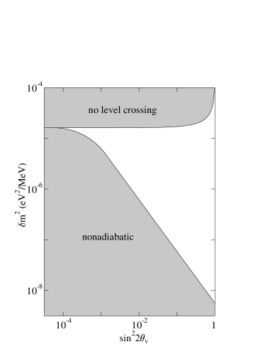
Figure 10: MSW conversion for a neutrino produced at the sun’s center. The upper shaded region indicates those $\delta m^{2}/E$ where the vacuum mass splitting is too great to be overcome by the solar density. Thus no level crossing occurs. The lower shaded region defines the region where the level crossing is non-adiabatic ($\gamma_{c}$ less than unity). The unshaded region corresponds to adiabatic level crossings where strong $\nu_{e}\rightarrow\nu_{\mu}$ will occur.

One can envision superimposing on Fig. 10 the spectrum of solar neutrinos, plotted as a function of ${\delta m^{2}\over E}$ for some choice of $\delta m^{2}$. Since Davis sees some solar neutrinos, the solutions must correspond to the boundaries of the triangle in Fig. 10. The horizontal boundary indicates the maximum ${\delta m^{2}\over E}$ for which the sun’s central density is sufficient to cause a level crossing. If a spectrum properly straddles this boundary, we obtain a result consistent with the Homestake experiment in which low energy neutrinos (large 1/E) lie above the level-crossing boundary (and thus remain $\nu_{e}$’s), but the high-energy neutrinos (small 1/E) fall within the unshaded region where strong conversion takes place. Thus such a solution would mimic nonstandard solar models in that only the ⁸B neutrino flux would be strongly suppressed. The diagonal boundary separates the adiabatic and non-adiabatic regions. If the spectrum straddles this boundary, we obtain a second solution in which low energy neutrinos lie within the conversion region, but the high-energy neutrinos (small 1/E) lie below the conversion region and are characterized by $\gamma\ll 1$ at the crossing density. (Of course, the boundary is not a sharp one, but is characterized by the Landau-Zener exponential). Such a non-adiabatic solution is quite distinctive since the flux of pp neutrinos, which is strongly constrained in the standard solar model and in any steady-state nonstandard model by the solar luminosity, would now be sharply reduced. Finally, one can imagine “hybrid” solutions where the spectrum straddles both the level-crossing (horizontal) boundary and the adiabaticity (diagonal) boundary for small $\theta$, thereby reducing the ⁷Be neutrino flux more than either the pp or ⁸B fluxes.

What are the results of a careful search for MSW solutions satisfying the Homestake, Kamiokande/SuperKamiokande, and SAGE/GALLEX constraints? This has been explored in detail by several groups. One solution, corresponding to a region surrounding $\delta m^{2}\sim 6\cdot 10^{-6}$eV² and $\sin^{2}2\theta_{v}\sim 6\cdot 10^{-3}$, is the hybrid case described above. It is commonly called the small-angle solution. A second, large-angle solution exists, corresponding to $\delta m^{2}\sim 10^{-5}$eV² and $\sin^{2}2\theta_{v}\sim$ 0.6. These solutions can be distinguished by their characteristic distortions of the solar neutrino spectrum. The survival probabilities $P_{\nu_{e}}^{\rm MSW}$(E) for the small- and large-angle parameters given above are shown as a function of E in Fig. 11.

Figure 11: MSW survival probabilities P(E_ν) for typical small angle and large angle solutions.

The MSW mechanism provides a natural explanation for the pattern of observed solar neutrino fluxes. While it requires profound new physics, both massive neutrinos and neutrino mixing are expected in extended models. The small-angle solution corresponds to $\delta m^{2}\sim 10^{-5}$ eV², and thus is consistent with $m_{2}\sim$ few $\cdot 10^{-3}$ eV. This is a typical $\nu_{\tau}$ mass in models where $m_{R}\sim m_{\rm{GUT}}$. This mass is also reasonably close to atmospheric neutrino values. On the other hand, if it is the $\nu_{\mu}$ participating in the oscillation, this gives $m_{R}\sim 10^{12}$ GeV and predicts a heavy $\nu_{\tau}\sim$ 10 eV. Such a mass is of great interest cosmologically as it would have consequences for supernova physics, the dark matter problem, and the formation of large-scale structure.

2.8 SuperKamiokande, SNO, and the MSW Mechanism

SuperKamiokande and Sudbury Neutrino Observatory (SNO) detectors are real-time counting detectors in contrast to the radiochemical detectors such as Homestake, GALLEX, and SAGE, which can only determine a time- and energy-integral of the flux (cf. Section 2.2). Both the SuperKamiokande and SNO can detect neutrinos through the reaction

$$\nu_{x}+e^{-}\rightarrow\nu_{x}+e^{-}.$$ (67)

The electrons coming from this reaction are confined to a forward cone. Hence detecting the Cerenkov radiation from the final electron one can determine neutrino’s direction. In this reaction it is very difficult to determine the energy of the neutrino from the measured energy of the final electron because of the kinematical broadening. However the measured energy spectra of the recoil electrons can nevertheless yield valuable information about the neutrino energy spectrum. Indeed recent SuperKamiokande measurement of the recoil electron energy spectrum is consistently below the SSM predictions at electron energies up to 14 MeV (which itself is consistent with other neutrino experiments). However for the higher energy bins the data are anomalously high as compared to the predictions. Although it can be fitted by assuming a very large hep neutrino flux $\!{}^{{\bf?}}$ the origin of this anomalous behavior is not understood.

In addition to the reaction Eq. (67) SNO can detect neutrinos through the charged-current reaction

$$\nu_{e}+d\rightarrow p+p+e^{-},$$ (68)

and the neutral current reaction

$$\nu_{x}(\overline{\nu}_{x})+d\rightarrow\nu_{x}(\overline{\nu}_{x})+p+n.$$ (69)

The neutrons produced in Eq. (69) can be detected either using $(n,\gamma)$ reactions on salt dissolved in the heavy water or by using ³He proportional counters. The electrons coming from the reaction (68) are essentially monochromatic with energies $\sim E_{\nu}-1.44$ MeV and they have a very different angular distribution ($1-\cos\theta_{e}/3$) with respect to the neutrino direction than that of the electrons coming from the reaction (67) (which are constrained to the forward cone).

It should be emphasized that since matter-enhanced neutrino conversion is energy-dependent, MSW mechanism will distort the neutrino energy spectra. However since only the energy of the final state electron can be measured, if a broad range of electron energies correspond to a given neutrino energy this distortion will be smeared. The charged current break-up reaction, Eq. (68), is more suitable for this purpose since the final electron energy is distributed around a very narrow peak centered at the initial neutrino energy. Spectrum distortion at SNO for the small-angle MSW solution ($\delta m^{2}\sim 5\times 10^{-6}$ eV² and $\sin 2\theta\sim 0.01$) is shown in Figure 12.

Figure 12: The dashed line shows the spectrum distortion at SNO for the small-angle MSW solution ($\delta m^{2}\sim 5\times 10^{-6}$ eV² and $\sin 2\theta\sim 0.01$). The solid line is the spectrum without MSW oscillations, normalized to the same total rate as with MSW oscillations.

The reaction (69) measures the total flux of all the neutrinos that participate in the low-energy weak interactions. Hence if there are no sterile neutrinos (more about this later) it can be used to test the neutrino oscillation hypothesis. For example if the electron neutrinos are being converted to muon neutrinos in the Sun, flux measured using the reaction (69) should agree with the SSM predictions. Finally it is worth mentioning that the electron antineutrinos coming from a supernova or a possible spin-flavor precession in the Sun (cf. Section 2.9) can also be detected through the reaction

$$\overline{\nu}_{e}+d\rightarrow n+n+e^{+}.$$ (70)

2.9 Other Particle Physics Solutions

If the MSW mechanism proves not to be the solution of the solar neutrino problem, it still will have greatly enhanced the importance of solar neutrino physics: the existing experiments have ruled out large regions in the $\delta m^{2}-\sin^{2}2\theta_{v}$ plane (corresponding to nearly complete $\nu_{e}\to\nu_{\mu}$ conversion) that remain hopelessly beyond the reach of accelerator neutrino oscillation experiments.

A number of other particle physics solutions have been considered, such as neutrino decay, matter-catalyzed neutrino decay, and solar energy transport by weakly interacting massive particles. But perhaps the most interesting possibility, apart from the MSW mechanism, was stimulated by suggestions that the ³⁷Cl signal might be varying with a period comparable to the 11-year solar cycle. While the evidence for this has weakened, the original claims generated renewed interest in neutrino magnetic moment interactions with the solar magnetic field.

The original suggestions by Cisneros and by Okun, Voloshyn, and Vysotsky envisioned the rotation

$$\nu_{e_{L}}\to\nu_{e_{R}}$$ (71)

producing a right-handed neutrino with sterile interactions in the standard model. With the discovery of the MSW mechanism, it was realized that matter effects would break the vacuum degeneracy of the $\nu_{e_{L}}$ and $\nu_{e_{R}}$, suppressing the spin precession. Lim and Marciano $\!{}^{{\bf?}}$ and Akhmedov $\!{}^{{\bf?}}$ pointed out that this difficulty was naturally circumvented for

$$\nu_{e_{L}}\to\nu_{\mu_{R}}$$ (72)

as the different matter interactions of the $\nu_{e}$ and $\nu_{\mu}$ can compensate for the vacuum $\nu_{e}-\nu_{\mu}$ mass difference, producing a crossing similar to the usual MSW mechanism. Such spin-flavor precession can then occur at full strength due to an off-diagonal (in flavor) magnetic moment.

Quite relevant to this suggestion is the very strong limit on both diagonal and off-diagonal magnetic moments is imposed by studies of the red giant cooling process of plasmon decay into neutrinos

$$\gamma^{*}\to\nu_{i}\bar{\nu}_{j}.$$ (73)

The result is $|\mu_{ij}|\mathrel{\hbox to0.0pt{\lower 4.0pt\hbox{\hskip 1.0pt$\sim$}\hss}\raise 1.0pt\hbox{$<$}}3\cdot 10^{-12}\mu_{B}$, where $\mu_{B}$ is an electron Bohr magneton $\!{}^{{\bf?}}$. (This can be compared to a simple one-loop estimate $\!{}^{{\bf?}}$ of the neutrino magnetic moment of $\sim 10^{-18}\mu_{B}$, taking a typical dark matter value for the neutrino mass of a few eV.) If a magnetic moment at the red giant limit is assumed, it follows that solar magnetic field strengths of $B_{\odot}\mathrel{\hbox to0.0pt{\lower 4.0pt\hbox{\hskip 1.0pt$\sim$}\hss}\raise 1.0pt\hbox{$>$}}10^{6}G$ are needed to produce interesting effects. Since the location of the spin-flavor level crossing depends on the neutrino energy, such fields have to be extensive to affect an appreciable fraction of the neutrino spectrum. It is unclear whether these conditions can occur in the sun.

We will return to a discussion of spin-flavor oscillations and associated effects later in these lectures. However, this brief introduction leads naturally to the next two topics, neutrino mass possibilities and the evolution of red giants.

3 Dirac and Majorana Neutrinos and Stellar Cooling

3.1 The Neutrino Mass Matrix

Consider a general 4n $\times$ 4n neutrino mass matrix where n is the number of flavors

$$\begin{array}[]{c}(\bar{\Psi}^{c}_{L},\bar{\Psi}^{R},\bar{\Psi}_{L},\bar{\Psi}^{c}_{R})\\ \\ \\ \end{array}\left(\begin{array}[]{cccc}0&0&M_{L}&M^{T}_{D}\\ 0&0&M_{D}&M_{R}^{\dagger}\\ M_{L}^{\dagger}&M_{D}^{\dagger}&0&0\\ M_{D}^{*}&M_{R}&0&0\end{array}\right)\left(\begin{array}[]{c}\Psi^{c}_{L}\\ \Psi_{R}\\ \Psi_{L}\\ \Psi^{c}_{R}\end{array}\right)$$ (74)

where each entry in this matrix is understood to be a n $\times$ n matrix operating in flavor space. The entries $M_{D}$ are the Dirac mass terms, while the $M_{L}$ and $M_{R}$ are the Majorana terms. The latter break the invariance of the Dirac equation under the transformation $\psi(x)\rightarrow e^{i\alpha}\psi(x)$ associated with a conserved lepton number. Thus it is these terms that govern lepton-number-violating processes like double beta decay.

One can proceed to diagonalize this matrix

$$\Psi_{\nu(e)}^{L}=\sum_{i=1}^{2n}U_{ei}^{L}\tilde{\nu}_{i}(x)~{}~{}\mathrm{with~{}masses}~{}m_{i}.$$ (75)

The eigenstates are two-component Majorana neutrinos $\!{}^{{\bf?}}$, yielding the proper $2\times 2n=4n$ degrees of freedom, where $n$ is the number of flavors. We can recover the Majorana and Dirac limits:
$\bullet$ If $M_{R}$ = $M_{L}$ = 0, the eigenstates of this matrix become pairwise degenerate, allowing the $2n$ two-component eigenstates to be paired to form $n$ four-component Dirac eigenstates.
$\bullet$ If $M_{D}$ = 0, the left- and right-handed components decouple, yielding $n$ left-handed Majorana eigenstates with standard model interactions.

There are interesting physical effects associated with these limits. Dirac neutrinos can have magnetic dipole, electric dipole (CP and T violating), and anapole (P violating) moments, as well as nonzero charge radii. Majorana neutrinos can have anapole moments but only transition magnetic and electric dipole moments. We mentioned in the previous lecture that transition magnetic moments were quite interesting in the context of MSW effects, as well as the use of $M_{R}$ in the seesaw mechanism.

In most extended models both Dirac and Majorana mass terms arise, with possibilities for interesting physics. We previously described the seesaw mechanism, which explains the lightness of the neutrinos as a effect of Dirac masses mixing with a heavy right-handed Majorana mass associated with scales far beyond the standard model. Another scenario often discussed in the pseudoDirac limit, where larger Dirac masses are accompanied by small Majorana masses. In the limit that the Majorana masses vanish, one recovers the degeneracy that allows one to patch two Majorana neutrinos with opposite CP into a four-component Dirac state, as described above. But if the Majorana terms remain non-vanishing, two Majorana states remain split by an amount $M_{L}$. If $M_{L}$ is much less than $M_{D}$, one obtains a nearly degenerate pair of states at mass $M_{D}$.

There are interesting low-energy consequences of these scenarios. Studies of the shape of the $\beta$ decay spectrum provides one test of neutrino masses: such tests are clearly limited to masses less than the Q-value of the decay. Since the different mass eigenstates correspond to distinct final states, the mass eigenstates do not interfere. Each neutrino that couples to the electron contributes to the decay according to its mixing probability $|U_{ei}|^{2}$ and according to the Fermi function $F(\omega_{e},m_{i})$, where $\omega_{e}$ is the electron energy and $m_{i}$ the mass of the $ith$ neutrino mass eigenstates. Thus massive neutrinos can appear as increments to the $\beta$ spectrum, turning on once $\omega_{e}$ drops below Q - $m_{i}$.

Another interesting process is neutrinoless double $\beta$ decay, which can be pictured as $\beta$ decay in which the produced neutrino is reabsorbed on a second nucleon, leading to a final state with no neutrinos and two electrons (and thus a nuclear charge change of two units). The neutrino mass eigenstates appear virtually, and thus clearly interfere. The process is also manifestly lepton-number violating, and thus must require Majorana masses. It can be shown that the amplitude, for light neutrino masses, depends on $|U_{ei}|^{2}m_{i}\eta^{CP}_{i}$, where $\eta^{CP}_{i}$ is the relative CP eigenvalue of the $ith$ mass eigenstate. (We are assuming CP conservation.) Thus in the Dirac limit, where the mass eigenstates of opposite CP become pairwise degenerate, this $\beta\beta$ decay mass vanishes. This then guarantees that the $\beta\beta$ amplitude vanishes in the absence of Majorana mass terms.

3.2 Red Giants and Helium Burning

We now consider the evolution off the main sequence of a solar-like star, with a mass above half a solar mass. As the hydrogen burning in the core progresses to the point that no more hydrogen is available, the stellar core consists of the ashes from this burning, ⁴He. The star then goes through an interesting evolution:
$\bullet$ With no further means of producing energy, the core slowly contracts, thereby increasing in temperature as gravity does work on the core.
$\bullet$ Matter outside the core is still hydrogen rich, and can generate energy through hydrogen burning. Thus burning in this shell of material supports the outside layers of the star. Note as the core contracts, this matter outside the core also is pulled deeper into the gravitational potential. Furthermore, the shell H burning continually adds more mass to the core. This means the burning in the shell must intensify to generate the additional gas pressure to fight gravity. The shell also thickens as this happens, since more hydrogen is above the burning temperature.
$\bullet$ The resulting increasing gas pressure causes the outer envelope of the star to expand by a larger factor, up to a factor of 50. The increase in radius more than compensates for the increased internal energy generation, so that a cooler surface results. The star reddens. Thus this class of star is named a red supergiant.
$\bullet$ This evolution is relatively rapid, perhaps a few hundred million years: the dense core requires large energy production. The helium core is supported by its degeneracy pressure, and is characterized by densities $\sim 10^{6}$ g/cm³. This stage ends when the core reaches densities and temperatures that allow helium burning through the reaction

$$\alpha+\alpha+\alpha\rightarrow^{12}C+\gamma.$$ (76)

As this reaction is very temperature dependent (see below), the conditions for ignition are very sharply defined. This has the consequence that the core mass at the helium flash point is well determined.
$\bullet$ The onset of helium burning produces a new source of support for the core. The energy release elevates the temperature and the core expands: He burning, not electron degeneracy, now supports the core. The burning shell and envelope have moved outward, higher in the gravitational potential. Thus shell hydrogen burning slows (the shell cools) because less gas pressure is needed to satisfy hydrostatic equilibrium. All of this means the evolution of the star has now slowed: the red giant moves along the “horizontal branch”, as interior temperatures slowly elevate much as in the main sequence.

The 3$\alpha$ process depends on some rather interesting nuclear physics. The first interesting “accident” involves the near degeneracy of the ⁸Be ground state and two separated $\alpha$s: The ⁸Be $0^{+}$ ground state is just 92 keV above the 2$\alpha$ threshold. The measured width of the ⁸Be ground state is 2.5 eV, which corresponds to a lifetime of

$$\tau_{m}\sim 2.6\cdot 10^{-16}\mathrm{s}.$$ (77)

One can compare this number to the typical time for one $\alpha$ to pass another. The red giant core temperature is $T_{7}\sim 10\rightarrow E\sim 8.6$ keV. Thus v/c $\sim$ 0.002. So the transit time is

$$\tau\sim{d\over v}\sim{5f\over 0.002}{1\over 3\cdot 10^{10}\mathrm{cm/sec}}{10^{-13}\mathrm{cm}\over f}\sim 8\cdot 10^{-21}\mathrm{s}.$$ (78)

This is more than five orders of magnitude shorter than $\tau_{m}$ above. Thus when a ⁸Be nucleus is produced, it lives for a substantial time compared to this naive estimate.

To quantify this, we calculate the flux-averaged cross section assuming resonant capture

$$\langle\sigma v\rangle=({2\pi\over\mu kT})^{3/2}{\Gamma\Gamma\over\Gamma}e^{-E_{r}/kT}$$ (79)

where $\Gamma$ is the 2$\alpha$ width of the ⁸Be ground state. This is the cross section for the $\alpha+\alpha$ reaction to form the compound nucleus then decay by $\alpha+\alpha$. But since there is only one channel, this is clearly also the result for producing the compound nucleus ⁸Be.

By multiplying the rate/volume for producing ⁸Be by the lifetime of ⁸Be, one gets the number of ⁸Be nuclei per unit volume

$$N(Be) = {N_{\alpha}N_{\alpha}\over 1+\delta_{\alpha\alpha}}\langle\sigma v\rangle\tau_{m}$$ (80)

$$= {N_{\alpha}N_{\alpha}\over 1+\delta_{\alpha\alpha}}\langle\sigma v\rangle{1\over\Gamma}$$

$$= {N_{\alpha}^{2}\over 2}({2\pi\over\mu kT})^{3/2}e^{-E_{r}/kT}.$$

Notice that the concentration is independent of $\Gamma$. So a small $\Gamma$ is not the reason we obtain a substantial buildup of ⁸Be. This is easily seen: if the width is small, then the production rate of ⁸Be goes down, but the lifetime of the nucleus once it is produced is longer. The two effects cancel to give the same ⁸Be concentration. One sees that the significant ⁸Be concentration results from two effects: 1) $\alpha+\alpha$ is the only open channel and 2) the resonance energy is low enough that some small fraction of the $\alpha+\alpha$ reactions have the requisite energy. As $E_{r}=92$ keV, $E_{r}/kT$ = 10.67/$T_{8}$ (where $T_{8}$ is the temperature in $10^{8}$K) so that

$$N(Be)=N_{\alpha}^{2}T_{8}^{-3/2}e^{-10.67/T_{8}}(0.94\cdot 10^{-33}\mathrm{cm^{3}}).$$ (81)

So plugging in typical values of $N_{\alpha}\sim 1.5\cdot 10^{28}$/cm³ (corresponding to $\rho_{\alpha}\sim 10^{5}$ g/cm³) and $T_{8}\sim$ 1 yields

$${N(^{8}Be)\over N(\alpha)}\sim 3.2\times 10^{-10}.$$ (82)

Salpeter suggested that this concentration would then allow $\alpha+^{8}$Be$\rightarrow^{12}$C to take place. Hoyle then argued that this reaction would not be fast enough to produce significant burning unless it was also resonant. Now the mass of ⁸Be + $\alpha$, relative to ¹²C,is 7.366 MeV, and each nucleus has $J^{\pi}=0^{+}$. Thus s-wave capture would require a $0^{+}$ resonance in ¹²C at $\sim$ 7.4 MeV. No such state was then known, but a search by Cook, Fowler, Lauritsen, and Lauritsen revealed a $0^{+}$ level at 7.644 MeV, with decay channels ⁸Be$+\alpha$ and $\gamma$ decay to the $2^{+}$ 4.433 level in ¹²C. The parameters are

$$\Gamma_{\alpha}\sim 8.9\mathrm{eV}~{}~{}~{}~{}~{}~{}~{}~{}\Gamma_{\gamma}\sim 3.6\cdot 10^{-3}\mathrm{eV}.$$ (83)

The resonant cross section formula gives

$$r_{48}=N_{8}N_{\alpha}({2\pi\over\mu kT})^{3/2}{\Gamma_{\alpha}\Gamma_{\gamma}\over\Gamma}e^{-E_{r}/kT}.$$ (84)

Plugging in our previous expression for $N(^{8}$Be) yields

$$r_{48}=N_{\alpha}^{3}T_{8}^{-3}e^{-42.9/T_{8}}(6.3\cdot 10^{-54}\mathrm{cm^{6}/s}).$$ (85)

If we denote by $\omega_{3\alpha}$ the decay rate of an $\alpha$ in our plasma, then

$$\omega_{3\alpha} = 3N_{\alpha}^{2}T_{8}^{-3}e^{-42.9/T_{8}}(6.3\cdot 10^{-54}\mathrm{cm^{6}/sec})$$ (86)

$$= ({N_{\alpha}\over 1.5\cdot 10^{28}/\mathrm{cm}^{3}})^{2}(4.3\cdot 10^{3}/\mathrm{sec})T_{8}^{-3}e^{-42.9/T_{8}}.$$

Now the energy release per reaction is 7.27 MeV. Thus we can calculate the energy produced per gram, $\epsilon$:

$$\epsilon = \omega_{3\alpha}{7.27\mathrm{MeV}\over 3}{1.5\cdot 10^{23}\over\mathrm{g}}$$ (87)

$$= (2.5\cdot 10^{21}\mathrm{erg/g~{}sec})({N_{\alpha}\over 1.5\cdot 10^{28}/\mathrm{cm}^{3}})^{2}T_{8}^{-3}e^{-42.9/T_{8}}.$$

We can evaluate this at a temperature of $T_{8}\sim$ 1 to find

$$\epsilon\sim(584\mathrm{ergs/g~{}sec})({N_{\alpha}\over 1.5\cdot 10^{28}/\mathrm{cm}^{3}})^{2}.$$ (88)

Typical values found in stellar calculations are in good agreement with this: typical red giant energy production is $\sim$ 100 ergs per gram per second.

To get a feel for the temperature sensitivity of this process, we can do a Taylor series expansion, finding

$$\epsilon(T)\sim({T\over T_{o}})^{40}N^{2}_{\alpha}.$$ (89)

This steep temperature dependence is the reason the He flash is delicately dependent on conditions in the core.

3.3 Neutrino Magnetic Moments and He Ignition

Prior to the helium flash, the degenerate He core radiates energy largely by neutrino pair emission. The process is the decay of a plasmon — which one can think of as a photon “dressed” by electron-hole excitations — thereby acquiring an effective mass of about 10 keV. The photon couples to a neutrino pair through a electron particle-hole pair that then decays into a $Z_{o}\rightarrow\nu\bar{\nu}$.

If this cooling is somehow enhanced, the degenerate helium core would be kept cooler, and would not ignite at the normal time. Instead it would continue to grow until it overcame the enhanced cooling to reach, once again, the ignition temperature.

One possible mechanism for enhanced cooling is a neutrino magnetic moment. Then the plasmon could directly couple to a neutrino pair. The strength of this coupling would depend on the size of the magnetic moment.

A delay in the time of He ignition has several observable consequences, including changing the ratio of red giant to horizontal branch stars. Thus, using the standard theory of red giant evolution, investigators have attempted to determine what size of magnetic moment would produce unacceptable changes in the astronomy. The result is a limit $\!{}^{{\bf?}}$ on the neutrino magnetic moment of

$$\mu_{ij}\mathrel{\hbox to0.0pt{\lower 4.0pt\hbox{\hskip 1.0pt$\sim$}\hss}\raise 1.0pt\hbox{$<$}}3\cdot 10^{-12}\mathrm{electron~{}Bohr~{}magnetons}$$ (90)

as was mentioned earlier. This limit is more than two orders of magnitude more stringent than that from direct laboratory tests.

This example is just one of a number of such constraints that can be extracted from similar stellar cooling arguments. The arguments above, for example, can be repeated for neutrino electric dipole moments. More interesting, it can be repeated for axion emission from red giants. Axions, the pseudoGolstone bosons associate with the solution of the strong CP problem suggested by Peccei and Quinn, are very light and can be produced radiatively within the red giant by the Compton process, by the Primakoff process off nuclei, or by emission from low-lying nuclear levels, such at from the 14 keV transition in ⁵⁷Fe. The net result is that axions of mass above a few eV are excluded; if axions have a direct coupling to electrons, so that the Compton process off electrons operates, the constraint is considerably tighter.

A similar argument can be formulated for supernova cooling. During SN1987A the neutrino burst detected by IMB and by Kamiokande was consistent with cooling on a timescale of about 4 seconds. Thus any process cooling the star more efficiently than neutrino emission would have shortened this time, while also reducing the flux in neutrinos. Large Dirac neutrino masses allow trapped neutrinos to scatter into sterile right-handed states. Right-handed neutrinos, lacking standard model interactions, would then escape the star (provided they do not scatter back into interacting left-handed states). Unfortunately the upper bounds imposed on the neutrino mass are quite model dependent, ranging over (1-25) keV.

The supernova cooling argument can also be repeated for axions. The window of sensitive runs from 1 eV (above this mass they are more strongly coupled than neutrinos, and thus cannot compete with neutrino cooling) to about 0.01 eV (below this mass they are too weakly coupled to be produced on the timescale of supernova cooling). It is interesting that the supernova and red giant cooling limit on axions nearly meet: a small window may still exist around a few eV if the axion has no coupling to electrons.

4 Atmospheric Neutrinos

Atmospheric neutrinos arise from the decay of secondary pions, kaons, and muons produced by the collisions of primary cosmic rays with the oxygen and nitrogen nuclei in the upper atmosphere. For energies less than 1 GeV all the secondaries decay :

$$\pi^{\pm}(K^{\pm}) \rightarrow \mu^{\pm}+\nu_{\mu}(\overline{\nu}_{\mu}),$$

$$\mu^{\pm} \rightarrow e^{\pm}+\nu_{e}(\overline{\nu}_{e})+\overline{\nu}_{\mu}(\nu_{\mu}).$$ (91)

Consequently one expects the ratio

$$r=(\nu_{e}+\overline{\nu}_{e})/(\nu_{\mu}+\overline{\nu}_{\mu})$$ (92)

to be approximately 0.5 in this energy range. Detailed Monte Carlo calculations $\!{}^{{\bf?}}$, including the effects of muon polarization, give $r\sim 0.45$. Since one is evaluating a ratio of similarly calculated processes, systematic errors are significantly reduced. Different groups estimating this ratio, even though they start with neutrino fluxes which can differ in magnitude by up to 25%, all agree within a few percent $\!{}^{{\bf?}}$. As the shower energy increases more muons survive due to time dilation. Hence one expects the ratio $r$ to decrease as the energy increases. The ratio (observed to predicted) of ratios

$$R={(\nu_{\mu}/\nu_{e})_{\rm data}\over(\nu_{\mu}/\nu_{e})_{\rm MonteCarlo}}$$ (93)

was determined in several experiments. There seems to be a persistent discrepancy between theory and experiment. The most recent measurement of this ratio at SuperKamiokande $\!{}^{{\bf?}}$ gives

$$R=0.63\pm 0.03({\rm stat})\pm 0.05({\rm syst})$$

for sub-GeV events which were fully contained in the detector and

$$R=0.65\pm 0.05({\rm stat})\pm 0.08({\rm syst})$$

for fully- and partially-contained multi-GeV events. As the agreement between data and theoretical expectation would give $R=1$, neutrino oscillations are invoked to explain the discrepancy. Another evidence for this explanation comes from measuring $R$ as a function of the zenith angle, $\Theta$, between the vertical and neutrino direction. A down-going neutrino ($\Theta\sim 0^{o}$) travels through the atmosphere above the detector (a distance of about 20 km), whereas an up-going neutrino ($\Theta\sim 180^{o}$) has traveled through the entire Earth (a distance of about 13000 km). Hence a measurement of number of neutrinos as a function of the zenith angle yields information about their numbers as a function of the distance traveled.

Figure 13: The ratio of fully contained events measured at SuperKamiokande versus reconstructed $L/E_{\nu}$. the dashed lines show the expected shape for $\nu_{\mu}\leftrightarrow\nu_{\tau}$ oscillations with $\delta m^{2}=2.2\cdot 10^{-3}$ eV² and $\sin^{2}2\theta=1$.

The SuperKamiokande collaboration measured the zenith angle dependence of not only $R$, but of the electron and muon neutrino fluxes separately $\!{}^{{\bf?}}$. This information is shown in Figure 13, where the data is plotted as a function of the reconstructed $L/E_{\nu}$ instead of the zenith angle. The data exhibit a zenith-angle (distance) dependent deficit of muon neutrinos, but not of electron neutrinos. This behavior is consistent with $\nu_{\mu}\leftrightarrow\nu_{\tau}$ oscillations. This interpretation is consistent with the recent measurements of up-going muons at Kamiokande $\!{}^{{\bf?}}$ and MACRO $\!{}^{{\bf?}}$ detectors. These muons are produced by the very high energy up-going muon neutrinos in the rocks surrounding the detectors. Both of these experiments also observe a deficit.

5 Supernovae, Supernova Neutrinos, and Nucleosynthesis

Consider a massive star, in excess of 10 solar masses, burning the hydrogen in its core under the conditions of hydrostatic equilibrium. When the hydrogen is exhausted, the core contracts until the density and temperature are reached where 3$\alpha\rightarrow^{12}$C can take place. The He is then burned to exhaustion. This pattern (fuel exhaustion, contraction, and ignition of the ashes of the previous burning cycle) repeats several times, leading finally to the explosive burning of ²⁸Si to Fe. For a heavy star, the evolution is rapid: the star has to work harder to maintain itself against its own gravity, and therefore consumes its fuel faster. A 25 solar mass star would go through all of these cycles in about 7 My, with the final explosive Si burning stage taking a few days. The result is an “onion skin” structure of the pre-collapse star in which the star’s history can be read by looking at the surface inward: there are concentric shells of H, ⁴He, ¹²C, ¹⁶O and ²⁰Ne, ²⁸Si, and ⁵⁶Fe at the center.

5.1 The Explosion Mechanism $\!{}^{{\bf?}}$

The source of energy for this evolution is nuclear binding energy. A plot of the nuclear binding energy $\delta$ as a function of nuclear mass shows that the minimum is achieved at Fe. In a scale where the ¹²C mass is picked as zero:

¹²C     $\delta$/nucleon = 0.000 MeV

¹⁶O     $\delta$/nucleon = -0.296 MeV

²⁸Si    $\delta$/nucleon = -0.768 MeV

⁴⁰Ca    $\delta$/nucleon = -0.871 MeV

⁵⁶Fe    $\delta$/nucleon = -1.082 MeV

⁷²Ge    $\delta$/nucleon = -1.008 MeV

⁹⁸Mo    $\delta$/nucleon = -0.899 Mev

Thus once the Si burns to produce Fe, there is no further source of nuclear energy adequate to support the star. So as the last remnants of nuclear burning take place, the core is largely supported by degeneracy pressure, with the energy generation rate in the core being less than the stellar luminosity. The core density is about 2 $\times 10^{9}$ g/cc and the temperature is kT $\sim$ 0.5 MeV.

Thus the collapse that begins with the end of Si burning is not halted by a new burning stage, but continues. As gravity does work on the matter, the collapse leads to a rapid heating and compression of the matter. As the nucleons in Fe are bound by about 8 MeV, sufficient heating can release $\alpha$s and a few nucleons. At the same time, the electron chemical potential is increasing. This makes electron capture on nuclei and any free protons favorable,

$$e^{-}+p\rightarrow\nu_{e}+n.$$ (94)

Note that the chemical equilibrium condition is

$$\mu_{e}+\mu_{p}=\mu_{n}+\langle E_{\nu}\rangle.$$ (95)

Thus the fact that neutrinos are not trapped plus the rise in the electron Fermi surface as the density increases, lead to increased neutronization of the matter. The escaping neutrinos carry off energy and lepton number. Both the electron capture and the nuclear excitation and disassociation take energy out of the electron gas, which is the star’s only source of support. This means that the collapse is very rapid. Numerical simulations find that the iron core of the star ($\sim$ 1.2-1.5 solar masses) collapses at about 0.6 of the free fall velocity.

In the early stages of the infall the $\nu_{e}$s readily escape. But neutrinos are trapped when a density of $\sim$ 10¹²g/cm³ is reached. At this point the neutrinos begin to scatter off the matter through both charged current and coherent neutral current processes. The neutral current neutrino scattering off nuclei is particularly important, as the scattering cross section is off the total nuclear weak charge, which is approximately the neutron number. This process transfers very little energy because the mass energy of the nucleus is so much greater than the typical energy of the neutrinos. But momentum is exchanged. Thus the neutrino “random walks” out of the star. When the neutrino mean free path becomes sufficiently short, the “trapping time” of the neutrino begins to exceed the time scale for the collapse to be completed. This occurs at a density of about 10¹² g/cm³, or somewhat less than 1% of nuclear density. After this point, the energy released by further gravitational collapse and the star’s remaining lepton number are trapped within the star.

If we take a neutron star of 1.4 solar masses and a radius of 10 km, an estimate of its binding energy is

$${GM^{2}\over 2R}\sim 2.5\times 10^{53}\mathrm{ergs}.$$ (96)

Thus this is roughly the trapped energy that will later be radiated in neutrinos.

The trapped lepton fraction $Y_{L}$ is a crucial parameter in the explosion physics: a higher trapped $Y_{L}$ leads to a larger homologous core, a stronger shock wave, and easier passage of the shock wave through the outer core, as will be discussed below. Most of the lepton number loss of an infalling mass element occurs as it passes through a narrow range of densities just before trapping. The reasons for this are relatively simple: on dimensional grounds weak rates in a plasma go as $T^{5}$, where T is the temperature. Thus the electron capture rapidly turns on as matter falls toward the trapping radius, and lepton number loss is maximal just prior to trapping. Inelastic neutrino reactions have an important effect on these losses, as the coherent trapping cross section goes as $E_{\nu}^{2}$ and is thus least effective for the lowest energy neutrinos. As these neutrinos escape, inelastic reactions repopulate the low energy states, allowing the neutrino emission to continue.

The velocity of sound in matter rises with increasing density. The inner homologous core, with a mass $M_{HC}\sim 0.6-0.9$ solar masses, is that part of the iron core where the sound velocity exceeds the infall velocity. This allows any pressure variations that may develop in the homologous core during infall to even out before the collapse is completed. As a result, the homologous core collapses as a unit, retaining its density profile. That is, if nothing were to happen to prevent it, the homologous core would collapse to a point.

The collapse of the homologous core continues until nuclear densities are reached. As nuclear matter is rather incompressible ($\sim$ 200 MeV/f³), the nuclear equation of state is effective in halting the collapse: maximum densities of 3-4 times nuclear are reached, e.g., perhaps $6\cdot 10^{14}$ g/cm³. The innermost shell of matter reaches this supernuclear density first, rebounds, sending a pressure wave out through the homologous core. This wave travels faster than the infalling matter, as the homologous core is characterized by a sound speed in excess of the infall speed. Subsequent shells follow. The resulting series of pressure waves collect near the sonic point (the edge of the homologous core). As this point reaches nuclear density and comes to rest, a shock wave breaks out and begins its traversal of the outer core.

Initially the shock wave may carry an order of magnitude more energy than is needed to eject the mantle of the star (less than 10⁵¹ ergs). But as the shock wave travels through the outer iron core, it heats and melts the iron that crosses the shock front, at a loss of $\sim$ 8 MeV/nucleon. The enhanced electron capture that occurs off the free protons left in the wake of the shock, coupled with the sudden reduction of the neutrino opacity of the matter (recall $\sigma_{coherent}\sim N^{2}$), greatly accelerates neutrino emission. This is another energy loss. The summed losses from shock wave heating and neutrino emission are comparable to the initial energy carried by the shock wave. Thus most numerical models fail to produce a successful “prompt” hydrodynamic explosion.

Most of the attention in the past decade focused on two explosion scenarios. In the prompt mechanism described above, the shock wave is sufficiently strong to survive the passage of the outer iron core with enough energy to blow off the mantle of the star. The most favorable results were achieved with smaller stars (less than 15 solar masses) where there is less overlying iron, and with soft equations of state, which produce a more compact neutron star and thus lead to more energy release. In part because of the lepton number loss problems discussed earlier, now it is widely believed that this mechanism fails for all but unrealistically soft nuclear equations of state.

The delayed mechanism begins with a failed hydrodynamic explosion; after about 0.01 seconds the shock wave stalls at a radius of 200-300 km. It exists in a sort of equilibrium, gaining energy from matter falling across the shock front, but loosing energy to the heating of that material. However, after perhaps 0.5 seconds, the shock wave is revived due to neutrino heating of the nucleon “soup” left in the wake of the shock. This heating comes primarily from charged current reactions off the nucleons in that nucleon gas; quasi-elastic scattering also contributes. This high entropy radiation-dominated gas may reach two MeV in temperature. The pressure exerted by this gas helps to push the shock outward. It is important to note that there are limits to how effective this neutrino energy transfer can be: if matter is too far from the core, the coupling to neutrinos is too weak to deposit significant energy. If too close, the matter may be at a temperature (or soon reach a temperature) where neutrino emission cools the matter as fast or faster than neutrino absorption heats it. The term “gain radius” is used to describe the region where useful heating is done.

This subject is still controversial and unclear. The problem is numerically challenging, forcing modelers to handle the difficult hydrodynamics of a shock wave; the complications of the nuclear equation of state at densities not yet accessible to experiment; modeling in two or three dimensions; handling the slow diffusion of neutrinos; etc. Not all of these aspects can be handled reasonably at the same time, even with existing supercomputers. Thus there is considerable disagreement about whether we have any supernova model that succeeds in ejecting the mantle.

However the explosion proceeds, there is agreement that 99% of the 3 $\cdot 10^{53}$ ergs released in the collapse is radiated in neutrinos of all flavors. The time scale over which the trapped neutrinos leak out of the protoneutron star is about three seconds. Through most of their migration out of the protoneutron star, the neutrinos are in flavor equilibrium

$$\mathrm{e.g.},~{}~{}\nu_{e}+\bar{\nu}_{e}\leftrightarrow\nu_{\mu}+\bar{\nu}_{\mu}.$$ (97)

As a result, there is an approximate equipartition of energy among the neutrino flavors. After weak decoupling, the $\nu_{e}$s and $\bar{\nu_{e}}$s remain in equilibrium with the matter for a longer period than their heavy-flavor counterparts, due to the larger cross sections for scattering off electrons and because of the charge-current reactions

$$\nu_{e}+n \leftrightarrow p+e^{-}$$

$$\bar{\nu_{e}}+p \leftrightarrow n+e^{+}.$$ (98)

Thus the heavy flavor neutrinos decouple from deeper within the star, where temperatures are higher. Typical calculations yield

$$T_{\nu_{\mu}}\sim T_{\nu_{\tau}}\sim 8\mathrm{MeV}~{}~{}~{}~{}T_{\nu_{e}}\sim 3.5\mathrm{MeV}~{}~{}~{}~{}T_{\bar{\nu_{e}}}\sim 4.5\mathrm{MeV}.$$ (99)

The difference between the $\nu_{e}$ and $\bar{\nu_{e}}$ temperatures is a result of the neutron richness of the matter, which enhances the rate for charge-current reactions of the $\nu_{e}$s, thereby keeping them coupled to the matter somewhat longer.

This temperature hierarchy is crucially important to nucleosynthesis and also to possible neutrino oscillation scenarios. The three-flavor MSW level-crossing diagram is shown in Fig. 14. One very popular scenario attributes the solar neutrino problem to $\nu_{\mu}\leftrightarrow\nu_{e}$ transmutation; this means that a second crossing with a $\nu_{\tau}$ could occur at higher density. It turns out plausible seesaw mass patterns suggest a $\nu_{\tau}$ mass on the order of a few eV, which would be interesting cosmologically. The second crossing would then occur outside the neutrino sphere, that is, after the neutrinos have decoupled and have fixed spectra with the temperatures given above. Thus a $\nu_{e}\leftrightarrow\nu_{\tau}$ oscillation would produce a distinctive $T\sim 8$ MeV spectrum of $\nu_{e}$s. This has dramatic consequences for terrestrial detection and for nucleosynthesis in the supernova.

Figure 14: Three-flavor neutrino level-crossing diagram. One popular scenario associates the solar neutrino problem with $\nu_{e}\leftrightarrow\nu_{\mu}$ oscillations and predicts a cosmologically interested massive $\nu_{\tau}$ with $\nu_{e}\leftrightarrow\nu_{\tau}$ oscillations near the supernova neutrinosphere.

5.2 The Neutrino Process $\!{}^{{\bf?}}$

Core-collapse supernovae are one of the major engines driving galactic chemical evolution, producing and ejecting the metals that enrich our galaxy. The discussion of the previous section described the hydrostatic evolution of a presupernova star in which large quantities of the most abundant metals (C, O, Ne,…) are synthesized and later ejected during the explosion. During the passage of the shock wave through the star’s mantle, temperature of $\sim(1-3)\cdot 10^{9}$K and are reached in the silicon, oxygen, and neon shells. This shock wave heating induces $(\gamma,\alpha)\leftrightarrow(\alpha,\gamma)$ and related reactions that generate a mass flow toward highly bound nuclei, resulting in the synthesis of iron peak elements as well as less abundant odd-A species. Rapid neutron-induced reactions are thought to take place in the high-entropy atmosphere just above the mass cut, producing about half of the heavy elements above A $\sim$ 80. This is the subject of the Sec. 4.3. Finally, the $\nu$-process described below is responsible for the synthesis of rare species such as ¹¹B and ¹⁹F. This process involves the response of nuclei at momentum transfers where the allowed approximation is no longer valid. Thus we will use the $\nu$-process in this section to illustrate some of the relevant nuclear physics.

One of the problems – still controversial – that may be connected with the neutrino process is the origin of the light elements Be, B and Li, elements which are not produced in sufficient amounts in the big bang or in any of the stellar mechanisms we have discussed. The traditional explanation has been cosmic ray spallation interactions with C, O, and N in the interstellar medium. In this picture, cosmic ray protons collide with C at relatively high energy, knocking the nucleus apart. So in the debris one can find nuclei like ¹⁰B, ¹¹B, and ⁷Li.

But there are some problems with this picture. First of all, this is an example of a secondary mechanism: the interstellar medium must be enriched in the C, O, and N to provide the targets for these reactions. Thus cosmic ray spallation must become more effective as the galaxy ages. The abundance of boron, for example, would tend to grow quadratically with metallicity, since the rate of production goes linearly with metallicity. But observations, especially recent measurements with the HST, find a linear growth $\!{}^{{\bf?}}$ in the boron abundance.

A second problem is that the spectrum of cosmic ray protons peaks near 1 GeV, leading to roughly comparable production of the two isotopes ¹⁰B and ¹¹B. That is, while it takes more energy to knock two nucleons out of carbon than one, this difference is not significant compared to typical cosmic ray energies. More careful studies lead to the expectation that the abundance ratio of ¹¹B to ¹⁰B might be $\sim$ 2. In nature, it is greater than 4.

Fans of cosmic ray spallation have offered solutions to these problems, e.g., similar reactions occurring in the atmospheres of nebulae involving lower energy cosmic rays. As this suggestion was originally stimulated by the observation of nuclear $\gamma$ rays from Orion, now retracted, some of the motivation for this scenario has evaporated. Here we focus on an alternative explanation, synthesis via neutrino spallation.

Previously we described the allowed Gamow-Teller (spin-flip) and Fermi weak interaction operators. These are the appropriate operators when one probes the nucleus at a wavelength – that is, at a size scale – where the nucleus responds like an elementary particle. We can then characterize its response by its macroscopic quantum numbers, the spin and charge. On the other hand, the nucleus is a composite object and, therefore, if it is probed at shorter length scales, all kinds of interesting radial excitations will result, analogous to the vibrations of a drumhead. For a reaction like neutrino scattering off a nucleus, the full operator involves the additional factor

$$e^{i\vec{k}\cdot\vec{r}}\sim 1+i\vec{k}\cdot\vec{r}$$ (100)

where the expression on the right is valid if the magnitude of $\vec{k}$ is not too large. Thus the full charge operator includes a “first forbidden” term

$$\sum_{i=1}^{A}\vec{r}_{i}\tau_{3}(i)$$ (101)

and similarly for the spin operator

$$\sum_{i=1}^{A}[\vec{r}_{i}\otimes\vec{\sigma}(i)]_{J=0,1,2}\tau_{3}(i).$$ (102)

These operators generate collective radial excitations, leading to the so-called “giant resonance” excitations in nuclei. The giant resonances are typically at an excitation energy of 20-25 MeV in light nuclei. One important property is that these operators satisfy a sum rule (Thomas-Reiche-Kuhn) of the form

$$\sum_{f}|\langle f|\sum_{i=1}^{A}r(i)\tau_{3}(i)|i\rangle|^{2}\sim{NZ\over A}\sim{A\over 4}$$ (103)

where the sum extends over a complete set of final nuclear states. These first-forbidden operators tend to dominate the cross sections for scattering the high energy supernova neutrinos ($\nu_{\mu}$s and $\nu_{\tau}$s), with $E_{\nu}\sim$ 25 MeV, off light nuclei. From the sum rule above, it follows that nuclear cross sections per target nucleon are roughly constant.

The E1 giant dipole mode described above is depicted qualitatively in Fig. 15a. This description, which corresponds to an early model of the giant resonance response by Goldhaber and Teller, involves the harmonic oscillation of the proton and neutron fluids against one another. The restoring force for small displacements would be linear in the displacement and dependent on the nuclear symmetry energy. There is a natural extension of this model to weak interactions, where axial excitations occur. For example, one can envision a mode similar to that of Fig. 15a where the spin-up neutrons and spin-down protons oscillate against spin-down neutrons and spin-up protons, the spin-isospin mode of Fig. 15b. This mode is one that arises in a simple SU(4) extension of the Goldhaber-Teller model, derived by assuming that the nuclear force is spin and isospin independent, at the same excitation energy as the E1 mode. In full, the Goldhaber-Teller model predicts a degenerate 15-dimensional supermultiplet of giant resonances, each obeying sum rules analogous to the TRK sum rule. While more sophisticated descriptions of the giant resonance region are available, of course, this crude picture is qualitatively accurate.

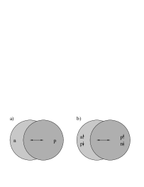
Figure 15: Schematic illustration of a) the E1 giant dipole mode familiar from electromagnetic interactions and b) a spin-isospin giant dipole mode associated with the first-forbidden weak axial response.

This nuclear physics is important to the $\nu$-process. The simplest example of $\nu$-process nucleosynthesis involves the Ne shell in a supernova. Because of the first-forbidden contributions, the cross section for inelastic neutrino scattering to the giant resonances in Ne is $\sim 3\cdot 10^{-41}$ cm²/flavor for the more energetic heavy-flavor neutrinos. This reaction

$$\nu+A\rightarrow\nu^{\prime}+A^{*}$$ (104)

transfers an energy typical of giant resonances, $\sim$ 20 MeV. A supernova releases about 3 $\times 10^{53}$ ergs in neutrinos, which converts to about $4\times 10^{57}$ heavy flavor neutrinos. The Ne shell in a 20 M_⊙ star has at a radius $\sim$ 20,000 km. Thus the neutrino fluence through the Ne shell is

$$\phi\sim{4\cdot 10^{57}\over 4\pi(20,000\mathrm{km})^{2}}\sim 10^{38}/\mathrm{cm}^{2}.$$ (105)

Thus folding the fluence and cross section, one concludes that approximately 1/300th of the Ne nuclei interact.

This is quite interesting since the astrophysical origin of ¹⁹F had not been understood. The only stable isotope of fluorine, ¹⁹F has an abundance

$${{}^{19}\mathrm{F}\over{}^{20}\mathrm{Ne}}\sim{1\over 3100}.$$ (106)

This leads to the conclusion that the fluorine found in a tube of toothpaste was created by neutral current neutrino reactions deep inside some ancient supernova.

The calculation of the final ¹⁹F/²⁰Ne ratio is more complicated than the simple 1/300 ratio given above:
$\bullet$ When Ne is excited by $\sim$ 20 MeV through inelastic neutrino scattering, it breaks up in two ways

$${}^{20}\mathrm{Ne}(\nu,\nu^{\prime})^{20}\mathrm{Ne}^{*} \rightarrow^{19}\mathrm{Ne}+n\rightarrow^{19}\mathrm{F}+e^{+}+\nu_{e}+n$$

$${}^{20}\mathrm{Ne}(\nu,\nu^{\prime})^{20}\mathrm{Ne}^{*} \rightarrow^{19}\mathrm{F}+p$$ (107)

with the first reaction occurring half as frequently as the second. As both channels lead to ¹⁹F, we have correctly estimated the instantaneous abundance ratio in the Ne shell of

$${{}^{19}\mathrm{F}\over{}^{20}\mathrm{Ne}}\sim{1\over 300}.$$ (108)

$\bullet$ We must also address the issue of whether the produced ¹⁹F survives. In the first 10^-8 sec the co-produced neutrons in the first reaction react via

$${}^{15}\mathrm{O}(n,p)^{15}\mathrm{N}~{}~{}^{19}\mathrm{Ne}(n,\alpha)^{16}\mathrm{O}~{}~{}^{20}\mathrm{Ne}(n,\gamma)^{21}\mathrm{Ne}~{}~{}^{19}\mathrm{Ne}(n,p)^{19}\mathrm{F}$$ (109)

with the result that about 70% of the ¹⁹F produced via spallation of neutrons is then immediate destroyed, primarily by the $(n,\alpha)$ reaction above. In the next $10^{-6}$ sec the co-produced protons are also processed

$${}^{15}\mathrm{N}(p,\alpha)^{12}\mathrm{C}~{}~{}^{19}\mathrm{F}(p,\alpha)^{16}\mathrm{O}~{}~{}^{23}\mathrm{Na}(p,\alpha)^{20}\mathrm{Ne}$$ (110)

with the latter two reactions competing as the primary proton poisons. This makes an important prediction: stars with high Na abundances should make more F, as the ²³Na acts as a proton poison to preserve the produced F.
$\bullet$ Finally, there is one other destruction mechanism, the heating associated with the passage of the shock wave. It turns out the the F produced prior to shock wave passage can survive if it is in the outside half of the Ne shell. The reaction

$${}^{19}\mathrm{F}(\gamma,\alpha)^{15}\mathrm{N}$$ (111)

destroys F for peak explosion temperatures exceeding $1.7\cdot 10^{9}$K. Such a temperature is produced at the inner edge of the Ne shell by the shock wave heating, but not at the outer edge.

If all of this physics in handled is a careful network code that includes the shock wave heating and F production both before and after shock wave passage, the following are the results:

$$\begin{array}[]{cc}\underline{[^{19}\mathrm{F}/^{20}\mathrm{Ne}]/[^{19}\mathrm{F}/^{20}\mathrm{Ne}]_{\odot}}&\underline{T_{\mathrm{heavy}~{}\nu}\mathrm{(MeV)}}\\ 0.14&4\\ 0.6&6\\ 1.2&8\\ 1.1&10\\ 1.1&12\end{array}$$

where the abundance ratio in the first column has been normalized to the solar value. One sees that the attribution of F to the neutrino process argues that the heavy flavor $\nu$ temperature must be greater than 6 MeV, a result theory favors. One also sees that F cannot be overproduced by this mechanism: although the instantaneous production of F continues to grow rapidly with the neutrino temperature, too much F results in its destruction through the $(p,\alpha)$ reaction, given a solar abundance of the competing proton poison ²³Na. Indeed, this illustrates an odd quirk: although in most cases the neutrino process is a primary mechanism, one needs ²³Na present to produce significant F. Thus in this case the neutrino process is a secondary mechanism.

While there are other significant neutrino process products (⁷Li, ¹³⁸La, ¹⁸⁰Ta, ¹⁵N …), the most important product is ¹¹B, produced by spallation off carbon. A calculation by Timmes et al.$\!{}^{{\bf?}}$ found that the combination of the neutrino process, cosmic ray spallation and big-bang nucleosynthesis together can explain the evolution of the light elements. The neutrino process, which produces a great deal of ¹¹B but relatively little ¹⁰B, combines with the cosmic ray spallation mechanism to yield the observed isotope ratio. Again, one prediction of this picture is that early stars should be ¹¹B rich, as the neutrino process is primary and operates early in our galaxy’s history; the cosmic ray production of ¹⁰B is more recent. There is hope that HST studies will soon be able to discriminate between ¹⁰B and ¹¹B: as yet this has not been done.

5.3 The r-process

Beyond the iron peak nuclear Coulomb barriers become so high that charged particle reactions become ineffective, leaving neutron capture as the mechanism responsible for producing the heaviest nuclei. If the neutron abundance is modest, this capture occurs in such a way that each newly synthesized nucleus has the opportunity to $\beta$ decay, if it is energetically favorable to do so. Thus weak equilibrium is maintained within the nucleus, so that synthesis is along the path of stable nuclei. This is called the s- or slow-process. However a plot of the s-process in the (N,Z) plane reveals that this path misses many stable, neutron-rich nuclei that are known to exist in nature. This suggests that another mechanism is at work, too. Furthermore, the abundance peaks found in nature near masses A $\sim$ 130 and A $\sim$ 190, which mark the closed neutron shells where neutron capture rates and $\beta$ decay rates are slower, each split into two sub-peaks. One set of sub-peaks corresponds to the closed-neutron-shell numbers N $\sim$ 82 and N $\sim$ 126, and is clearly associated with the s-process. The other set is shifted to smaller N, $\sim$ 76 and $\sim$ 116, respectively, and is suggestive of a much more explosive neutron capture environment where neutron capture can be rapid.

This second process is the r- or rapid-process, characterized by:
$\bullet$ The neutron capture is fast compared to $\beta$ decay rates.
$\bullet$ The equilibrium maintained within a nucleus is established by $(n,\gamma)\leftrightarrow(\gamma,n)$: neutron capture fills up the available bound levels in the nucleus until this equilibrium sets in. The new Fermi level depends on the temperature and the relative $n/\gamma$ abundance.
$\bullet$ The nucleosynthesis rate is thus controlled by the $\beta$ decay rate: each $\beta^{-}$ capture converting n $\rightarrow$ p opens up a hole in the neutron Fermi sea, allowing another neutron to be captured.
$\bullet$ The nucleosynthesis path is along exotic, neutron-rich nuclei that would be highly unstable under normal laboratory conditions.
$\bullet$ As the nucleosynthesis rate is controlled by the $\beta$ decay, mass will build up at nuclei where the $\beta$ decay rates are slow. It follows, if the neutron flux is reasonable steady over time so that equilibrated mass flow is reached, that the resulting abundances should be inversely proportional to these $\beta$ decay rates.

Let’s first explore the $(n,\gamma)\leftrightarrow(\gamma,n)$ equilibrium condition, which requires that the rate for $(n,\gamma)$ balances that for $(\gamma,n)$ for an average nucleus. So consider the formation cross section

$$A+n\rightarrow(A+1)+\gamma.$$ (112)

This is an exothermic reaction, as the neutron drops into the nuclear well. Our averaged cross section, assuming a resonant reaction (the level density is high in heavy nuclei) is

$$\langle\sigma v\rangle_{(n,\gamma)}=\left({2\pi\over\mu kT}\right)^{3/2}{\Gamma_{n}\Gamma_{\gamma}\over\Gamma}e^{-E/KT}$$ (113)

where E $\sim$ 0 is the resonance energy, and the $\Gamma$s are the indicated partial and total widths. Thus the rate per unit volume is

$$r_{(n,\gamma)}\sim N_{n}N_{A}\left({2\pi\over\mu kT}\right)^{3/2}{\Gamma_{n}\Gamma_{\gamma}\over\Gamma}$$ (114)

where $N_{n}$ and $N_{A}$ are the neutron and nuclear number densities and $\mu$ the reduced mass. This has to be compared to the $(\gamma,n)$ rate.

The $(\gamma,n)$ reaction requires the photon number density in the gas. This is given by the Bose-Einstein distribution

$$N(\epsilon)={8\pi\over c^{3}h^{3}}{\epsilon^{2}d\epsilon\over e^{\epsilon/kT}-1}.$$ (115)

The high-energy tail of the normalized distribution can thus be written

$$\sim{1\over N_{\gamma}\pi^{2}}\epsilon^{2}e^{-\epsilon/kT}d\epsilon$$ (116)

where in the last expression we have set $\hbar=c=1$.

Now we need the resonant cross section in the $(\gamma,n)$ direction. For photons the wave number is proportional to the energy, so

$$\sigma_{(\gamma,n)}={\pi\over\epsilon^{2}}{\Gamma_{\gamma}\Gamma_{n}\over(\epsilon-E_{r})^{2}+(\Gamma/2)^{2}}.$$ (117)

As the velocity is c =1,

$$\langle\sigma v\rangle={1\over\pi^{2}N_{\gamma}}\int_{0}^{\infty}\epsilon^{2}e^{-\epsilon/kT}d\epsilon{\pi\over\epsilon^{2}}{\Gamma_{\gamma}\Gamma_{n}\over(\epsilon-E_{r})^{2}+(\Gamma/2)^{2}}.$$ (118)

We evaluate this in the usual way for a sharp resonance, remembering that the energy integral over just the denominator above (the sharply varying part) is $2\pi/\Gamma$

$$\sim{\Gamma_{\gamma}\Gamma_{n}\over N_{\gamma}}e^{-E_{r}/kT}{2\over\Gamma}.$$ (119)

So that the rate becomes

$$r_{(\gamma,n)}\sim 2N_{A+1}{\Gamma_{\gamma}\Gamma_{n}\over\Gamma}e^{-E_{r}/kT}.$$ (120)

Equating the $(n,\gamma)$ and $(\gamma,n)$ rates and taking $N_{A}\sim N_{A-1}$ then yields

$$N_{n}\sim{2\over(\hbar c)^{3}}\left({\mu c^{2}kT\over 2\pi}\right)^{3/2}e^{-E_{r}/kT}$$ (121)

where the $\hbar$s and $c$s have been properly inserted to give the right dimensions. Now $E_{r}$ is essentially the binding energy. So plugging in the conditions $N_{n}\sim 3\times 10^{23}$/cm³ and $T_{9}\sim 1$, we find that the binding energy is $\sim$ 2.4 MeV. Thus neutrons are bound by about 30 times $kT$, a value that is still small compared to a typical binding of 8 MeV for a normal nucleus. (In this calculation the neutron reduced mass is calculated by assuming a nuclear target with A=150.)

The above calculation fails to count spin states for the photons and nuclei and is thus not quite correct. But it makes the essential point: the r-process involves very exotic species largely unstudied in any terrestrial laboratory. It is good to bear this in mind, as in the following section we will discuss the responses of such nuclei to neutrinos. Such responses thus depend on the ability of theory to extrapolate responses from known nuclei to those quite unfamiliar.

The path of the r-process is along neutron-rich nuclei, where the neutron Fermi sea is just $\sim$ (2-3) MeV away from the neutron drip line (where no more bound neutron levels exist). After the r-process finishes (the neutron exposure ends) the nuclei decay back to the valley of stability by $\beta$ decay. This can involve some neutron spallation ($\beta$-delayed neutrons) that shift the mass number A to a lower value. But it certainly involves conversion of neutrons into protons, and that shifts the r-process peaks at N $\sim$ 82 and 126 to a lower N, off course. This effect is clearly seen in the abundance distribution: the r-process peaks are shifted to lower N relative to the s-process peaks. This is the origin of the second set of “sub-peaks” mentioned at the start of the section.

It is believed that the r-process can proceed to very heavy nuclei (A $\sim$ 270) where it is finally ended by $\beta$-delayed and n-induced fission, which feeds matter back into the process at an A $\sim$ A_max/2. Thus there may be important cycling effects in the upper half of the r-process distribution.

What is the site(s) of the r-process? This has been debated many years and still remains a controversial subject:
$\bullet$ The r-process requires exceptionally explosive conditions

$\rho$(n) $\sim 10^{20}$ cm^-3   T $\sim 10^{9}$K   t $\sim$ 1s.

$\bullet$ Both primary and secondary sites proposed. Primary sites are those not requiring preexisting metals. Secondary sites are those where the neutron capture occurs on preexisting s-process seeds.
$\bullet$ Suggested primary sites include the the neutronized atmosphere above the proto-neutron star in a Type II supernova, neutron-rich jets produced in supernova explosions or in neutron star mergers, inhomogeneous big bangs, etc.
$\bullet$ Secondary sites, where $\rho$(n) can be lower for successful synthesis, include the He and C zones in Type II supernovae, the red giant He flash, etc.

The balance of evidence favors a primary site, so one requiring no pre-enrichment of heavy s-process metals. Among the evidence:

1) HST studies of very-metal-poor halo stars: The most important evidence are the recent HST measurements of Cowan, Sneden et al. $\!{}^{{\bf?}}$ of very metal-poor stars ([Fe/H] $\sim$ -1.7 to -3.12) where an r-process distribution very much like that of our sun has been seen for Z $\mathrel{\hbox to0.0pt{\lower 4.0pt\hbox{\hskip 1.0pt$\sim$}\hss}\raise 1.0pt\hbox{$>$}}$ 56. Furthermore, in these stars the iron content is variable. This suggests that the “time resolution” inherent in these old stars is short compared to galactic mixing times (otherwise Fe would be more constant). The conclusion is that the r-process material in these stars is most likely from one or a few local supernovae. The fact that the distributions match the solar r-process (at least above charge 56) strongly suggests that there is some kind of unique site for the r-process: the solar r-process distribution did not come from averaging over many different kinds of r-process events. Clearly the fact that these old stars are enriched in r-process metals also strongly argues for a primary process: the r-process works quite well in an environment where there are few initial s-process metals.

2) There are also fairly good theoretical arguments that a primary r-process occurring in a core-collapse supernova might be viable $\!{}^{{\bf?}}$. First, galactic chemical evolution studies indicate that the growth of r-process elements in the galaxy is consistent with low-mass Type II supernovae in rate and distribution. More convincing is the fact that modelers have shown that the conditions needed for an r-process (very high neutron densities, temperatures of 1-3 billion degrees) might be realized in a supernova. The site is the last material expelled from the supernova, the matter just above the mass cut. When this material is blown off the star initially, it is a very hot neutron-rich, radiation-dominated gas containing neutrons and protons, but an excess of the neutrons. As it expands off the star and cools, the material first goes through a freeze-out to $\alpha$ particles, a step that essentially locks up all the protons in this way. Then the $\alpha$s interact through reactions like

$$\alpha+\alpha+\alpha \rightarrow^{12}C$$

$$\alpha+\alpha+n \rightarrow^{9}Be$$

to start forming heavier nuclei. Note, unlike the big bang, that the density is high enough to allow such three-body interactions to bridge the mass gaps at A = 5,8. The $\alpha$ capture continues up to heavy nuclei, to A $\sim$ 80, in the network calculations. The result is a small number of “seed” nuclei, a large number of $\alpha$s, and excess neutrons. These neutrons preferentially capture on the heavy seeds to produce an r-process. Of course, what is necessary is to have $\sim$ 100 excess neutrons per seed in order to successfully synthesize heavy mass nuclei. Some of the modelers find conditions where this almost happens.

There are some very nice aspects of this site: the amount of matter ejected is about 10${}^{-5}-10^{-6}$ solar masses, which is just about what is needed over the lifetime of the galaxy to give the integrated r-process metals we see, taking a reasonable supernova rate. But there are also a few problems, especially the fact that with calculated entropies in the nucleon soup above the proto-neutron star, neutron fractions appear to be too low to produce a successful A $\sim$ 190 peak. There is some interesting recent work invoking neutrino oscillations to cure this problem: charge current reactions on free protons and neutrons determine the n/p ratio in the gas. Then, for example, an oscillation of the type $\nu_{e}\rightarrow\nu_{\mathrm{sterile}}$ can alter this ratio, as it would turn off the $\nu_{e}$s that destroy neutrons by charged-current reactions$\!{}^{{\bf?}}$. Unfortunately, a full discussion of such possibilities would take us too far afield today.

The nuclear physics of the r-process tells us that the synthesis occurs when the nucleon soup is in the temperature range of (3-1) $\cdot 10^{9}$K, which, in the hot bubble r-process described above, corresponds to a freeze-out radius of (600-100) km and a time $\sim$ 10 seconds after core collapse. The neutrino fluence after freeze-out (when the temperature has dropped below 10⁹K and the r-process stops) is then $\sim$ (0.045-0.015) $\cdot 10^{51}$ ergs/(100km). Thus, after completion of the r-process, the newly synthesized material experiences an intense flux of neutrinos. This brings up the question of whether the neutrino flux could have any effect on the r-process.

5.4 Neutrinos and the r-process $\!{}^{{\bf?}}$

Rather than describe the exotic effects of neutrino oscillations on the r-process, mentioned briefly above, we will examine standard-model effects that are nevertheless quite interesting. The nuclear physics of this section – neutrino-induced neutron spallation reactions – is also relevant to recently proposed supernova neutrino observatories such as OMNIS and LAND. In contrast to our first discussion of the $\nu$-process in Sec. 4.2, it is apparent that neutrino effects could be much larger in the hot bubble r-process: the synthesis occurs much closer to the star than our Ne radius of 20,000 km: estimates are 600-1000 km. The r-process is completed in about 10 seconds (when the temperature drops to about one billion degrees), but the neutrino flux is still significant as the r-process freezes out. The net result is that the “post-processing” neutrino fluence - the fluence that can alter the nuclear distribution after the r-process is completed - is about 100 times larger than that responsible for fluorine production in the Ne zone. Recalling that 1/300 of the nuclei in the Ne zone interacted with neutrinos, and remembering that the relevant neutrino-nucleus cross sections scale as A, one quickly sees that the probability of a r-process nucleus interacting with the neutrino flux is approximately unity.

Because the hydrodynamic conditions of the r-process are highly uncertain, one way to attack this problem is to work backward in time. We know the final r-process distribution (what nature gives us) and we can calculate neutrino-nucleus interactions relatively well. Thus from the observed r-process distribution (including neutrino post-processing) we can work backward to find out what the r-process distribution looked like at the point of freeze-out. In Figs. 16 and 17, the “real” r-process distribution - that produced at freeze-out - is given by the dashed lines, while the solid lines show the effects of the neutrino post-processing for a particular choice of fluence. The nuclear physics input into these calculations is precisely that previously described: GT and first-forbidden cross sections, with the responses centered at excitation energies consistent with those found in ordinary, stable nuclei, taking into account the observed dependence on $|N-Z|$.

Figure 16: Comparison of the r-process distribution that would result from the freeze-out abundances near the A $\sim$ 130 mass peak (dashed line) to that where the effects of neutrino post-processing have been include (solid line). The fluence has been fixed by assuming that the A = 124-126 abundances are entirely due to the $\nu$-process.

One important aspect of the figures is that the mass shift is significant. This has to do with the fact that a 20 MeV excitation of a neutron-rich nucleus allows multiple neutrons ( $\sim$ 5) to be emitted. (Remember we found that the binding energy of the last neutron in an r-process neutron-rich nuclei was about 2-3 MeV under typical r-process conditions.) The second thing to notice is that the relative contribution of the neutrino process is particularly important in the “valleys” beneath the mass peaks: the reason is that the parents on the mass peak are abundant, and the valley daughters rare. In fact, it follows from this that the neutrino process effects can be dominant for precisely seven isotopes (Te, Re, etc.) lying in these valleys. Furthermore if an appropriate neutrino fluence is picked, these isotope abundances are produced perfectly (given the abundance errors). The fluences are

$$\mathrm{N} = 82~{}\mathrm{peak}~{}~{}~{}~{}~{}0.031\cdot 10^{51}\mathrm{ergs/(100km)^{2}/flavor}$$

$$\mathrm{N} = 126~{}\mathrm{peak}~{}~{}~{}~{}0.015\cdot 10^{51}\mathrm{ergs/(100km)^{2}/flavor},$$

values in fine agreement with those that would be found in a hot bubble r-process. So this is circumstantial but significant evidence that the material near the mass cut of a Type II supernova is the site of the r-process: there is a neutrino fingerprint.

Figure 17: As in Fig. 16, but for the A $\sim$ 195 mass peak. The A = 183-187 abundances are entirely attributed to the $\nu$-process.

In the following sections we will briefly return to the effects of supernova density and electron fraction fluctuations and sterile neutrino mixings on the supernova r-process.

6 MSW Exotica

6.1 Spin-Flavor Oscillations

In section 2.9 we briefly touched upon the effects of neutrino magnetic moment on neutrino propagation through matter. The chiral components of neutrino propagating in matter satisfy the equation $\!{}^{{\bf?}}$

$$i\frac{\partial}{\partial t}\left[\begin{array}[]{cc}\nu_{L}\\ \\ \nu_{R}\end{array}\right]=\left[\begin{array}[]{cc}\frac{G_{F}}{\sqrt{2}}(2N_{e}-N_{n})&\mu B\\ \\ \mu B&0\end{array}\right]\left[\begin{array}[]{cc}\nu_{L}\\ \\ \nu_{R}\end{array}\right]\,,$$ (122)

where $N_{e}$ and $N_{n}$ are the electron and neutron densities in the media, respectively. As Eq. (122) demonstrates the chiral rotation is actually suppressed in matter. It was soon realized $\!{}^{{\bf?}}$, however, that combining the chiral precession and the MSW flavor transformation by including non-diagonal magnetic moments circumvents this problem. One then should consider the evolution of left- and right-handed components of the electron and muon neutrinos together:

$$i\frac{\partial}{\partial t}\left[\begin{array}[]{c}\nu_{e}^{L}\\ \nu_{\mu}^{L}\\ \nu_{e}^{R}\\ \nu{{}_{\mu}}^{R}\end{array}\right]=\left[\begin{array}[]{cc}H_{L}&BM^{\dagger}\\ \\ BM&H_{R}\end{array}\right]\left[\begin{array}[]{c}\nu_{e}^{L}\\ \nu_{\mu}^{L}\\ \nu_{e}^{R}\\ \nu{{}_{\mu}}^{R}\end{array}\right].$$ (123)

For Dirac neutrinos the block matrices appearing in the evolution Hamiltonian in Eq. (123) are given by

$$H_{L}=\left[\begin{array}[]{cc}\frac{\delta m^{2}}{2E}\sin^{2}{\theta_{v}}+\frac{G_{F}}{\sqrt{2}}(2N_{e}-N_{n})&\frac{\delta m^{2}}{4E}\sin{2\theta_{v}}\\ \\ \frac{\delta m^{2}}{4E}\sin{2\theta_{v}}&\frac{\delta m^{2}}{2E}\sin^{2}{\theta_{v}}-\frac{G_{F}}{\sqrt{2}}N_{n}\end{array}\right],$$ (124)

$$H_{R}=\left[\begin{array}[]{cc}\frac{\delta m^{2}}{2E}\sin^{2}{\theta_{v}}&\frac{\delta m^{2}}{4E}\sin{2\theta_{v}}\\ \\ \frac{\delta m^{2}}{4E}\sin{2\theta_{v}}&\frac{\delta m^{2}}{2E}\sin^{2}{\theta_{v}}\end{array}\right],$$ (125)

and

$$M=\left[\begin{array}[]{cc}\mu_{ee}&\mu_{e\mu}\\ \\ \mu_{\mu e}&\mu_{\mu\mu}\end{array}\right].$$ (126)

In these equations $B$ is the component of the magnetic field transverse to the direction of neutrino propagation. The last equation contains both diagonal and transition magnetic moments for neutrinos. For Majorana neutrinos diagonal moments vanish and, since neutrinos are their own antiparticles, both left-handed and right-handed neutrinos must mix with the same mixing matrix. Hence for Majorana neutrinos the evolution matrix takes the form

$$\left[\begin{array}[]{cccc}\frac{G_{F}}{\sqrt{2}}(2N_{e}-N_{n})&\frac{\delta m^{2}}{4E}\sin{2\theta_{v}}&0&\mu^{*}B\\ \\ \\ \\ \frac{\delta m^{2}}{4E}\sin{2\theta_{v}}&\frac{\delta m^{2}}{2E}\cos{2\theta_{v}}-\frac{G_{F}}{\sqrt{2}}N_{n}&-\mu^{*}B&0\\ \\ \\ \\ 0&-\mu B&-\frac{G_{F}}{\sqrt{2}}(2N_{e}-N_{n})&\frac{\delta m^{2}}{4E}\sin{2\theta_{v}}\\ \\ \\ \\ \mu B&0&\frac{\delta m^{2}}{4E}\sin{2\theta_{v}}&\frac{\delta m^{2}}{2E}\cos{2\theta_{v}}+\frac{G_{F}}{\sqrt{2}}N_{n}\end{array}\right].$$ (127)

These evolution equations were numerically investigated in detail both for the Sun $\!{}^{{\bf?}}$ and supernovae $\!{}^{{\bf?}}$. This was motivated by the Homestake data which suggested an anti-correlation between sunspot number and the capture rate of solar neutrinos. It is rather difficult to understand such a behavior in a theoretical framework since the most straightforward explanation for short-term time-variation of the neutrino flux is to assume the existence of a rather large neutrino magnetic moment, inconsistent with the bounds discussed in Section 3.3. Also Kamiokande and SuperKamiokande solar neutrino data do not show such time-variations.

6.2 Neutrino Propagation in Stochastic Media

In implementing the MSW solution to the solar neutrino problem one typically assumes that the electron density of the Sun is a monotonically decreasing function of the distance from the core and ignores potentially de-cohering effects $\!{}^{{\bf?}}$. To understand such effects one possibility is to study parametric changes in the density or the role of matter currents $\!{}^{{\bf?}}$. In this regard, Loreti and Balantekin $\!{}^{{\bf?}}$ considered neutrino propagation in stochastic media. They studied the situation where the electron density in the medium has two components, one average component given by the Standard Solar Model or Supernova Model, etc. and one fluctuating component. Then the Hamiltonian in Eq. (53) takes the form

$$\hat{H}=\left({{-\delta m^{2}}\over 4E}\cos 2\theta+{1\over\sqrt{2}}G_{F}(N_{e}(r)+N^{r}_{e}(r))\right){\sigma_{z}}+\left({{\delta m^{2}}\over 4E}\sin 2\theta\right){\sigma_{x}}.$$ (128)

where one imposes for consistency

$$\langle N^{r}_{e}(r)\rangle=0,$$ (129)

and a two-body correlation function

$$\langle N^{r}_{e}(r)N^{r}_{e}(r^{\prime})\rangle={\beta}^{2}\ N_{e}(r)\ N_{e}(r^{\prime})\ \exp(-|r-r^{\prime}|/\tau_{c}).$$ (130)

Figure 18: Mean electron neutrino survival probability in the sun with fluctuations. The average electron density is given by the Standard Solar Model of Bahcall and Pinsonneault and $\sin^{2}2\theta=0.01$.

In the calculations of the Wisconsin group the fluctuations are typically taken to be subject to colored noise, i.e. higher order correlations

$$f_{12\cdots}=\langle N^{r}_{e}(r_{1})N^{r}_{e}(r_{2})\cdots\rangle$$ (131)

are taken to be

$$f_{1234}=f_{12}f_{34}+f_{13}f_{24}+f_{14}f_{23},$$ (132)

and so on.

The mean survival probability $\!{}^{{\bf?}}$ for the electron neutrino in the Sun is shown in Figure 18 where fluctuations are imposed on the average solar electron density given by the Bahcall-Pinsonneault model. One notes that for very large fluctuations complete flavor de-polarization should be achieved, i.e. the neutrino survival probability is 0.5, the same as the vacuum oscillation probability for long distances. To illustrate this behavior the results from the physically unrealistic case of 50% fluctuations are shown. Also the effect of the fluctuations is largest when the neutrino propagation in their absence is adiabatic. This scenario was applied to the neutrino convection in a core-collapse supernova where the adiabaticity condition is satisfied $\!{}^{{\bf?}}$. Similar results were also obtained by other authors $\!{}^{{\bf?}}$. It may be possible to test solar matter density fluctuations at the BOREXINO detector currently under construction $\!{}^{{\bf?}}$. Propagation of a neutrino with a magnetic moment in a random magnetic moment has also been investigated $\!{}^{{\bf?},{\bf?}}$. Also if the magnetic field in a polarized medium has a domain structure with different strength and direction in different domains, the modification of the potential felt by the neutrinos due polarized electrons will have a random character $\!{}^{{\bf?}}$. Using the formalism sketched above, it is possible to calculate not only the mean survival probability, but also the variance, $\sigma$, of the fluctuations to get a feeling for the distribution of the survival probabilities $\!{}^{{\bf?}}$ as illustrated in Figure 19.

Figure 19: Mean electron neutrino survival probability plus minus $\sigma$ in the sun with fluctuations. The average electron density is given by the Standard Solar Model of Bahcall and Pinsonneault and $\sin^{2}2\theta=0.01$. Panels (a), (b), (c), and (d) correspond to an average fluctuation of 1%, 2%, 4%, and 8% respectively.

In these calculations the correlation length $\tau$ is taken to be very small, of the order of 10 km., to be consistent with the helioseismic observations of the sound speed (cf. Section 2.5). In the opposite limit of very large correlation lengths are very interesting result is obtained $\!{}^{{\bf?}}$, namely the averaged density matrix is given as an integral

$$\lim_{\tau_{c}\to\infty}\langle\hat{\rho}(r)\rangle={1\over{\sqrt{2\pi\beta^{2}}}}\int_{-\infty}^{\infty}dx\exp[{-x^{2}/(2\beta^{2})}]\hat{\rho}(r,x),$$ (133)

reminiscent of the channel-coupling problem in nuclear physics $\!{}^{{\bf?}}$. Even though this limit is not appropriate to the solar fluctuations it may be applicable to a number of other astrophysical situations.

6.3 Approximate Solutions and Neutrino Tomography

Exact solutions for the neutrino propagation equations in matter exist only for a limited class of density profiles. For example, for those density profiles that satisfy an integrability condition called shape invariance neutrino survival probability can be found with algebraic methods $\!{}^{{\bf?}}$. One can also use various approximation methods to solve Eq. (53). The standard semi-classical approximation gives the adiabatic evolution $\!{}^{{\bf?}}$. For a monotonically changing density profile supersymmetric uniform approximation yields $\!{}^{{\bf?}}$ the hopping probability of Eq. (65) to be

$$P_{hop} = \exp(-\pi\Omega),$$

$$\Omega = \frac{i}{\pi}\frac{\delta m^{2}}{2E}\int^{r_{0}^{*}}_{r_{0}}dr\left[\zeta^{2}(r)-2\zeta(r)\cos{2\theta_{v}}+1\right]^{1/2}\,,$$ (134)

where ${r_{0}^{*}}$ and ${r_{0}}$ are the turning points (zeros) of the integrand. In this expression we introduced the scaled density

$$\zeta(r)=\frac{2\sqrt{2}G_{F}N_{e}(r)}{\delta m^{2}/E}\,,$$ (135)

where $N_{e}$ is the number density of electrons in the medium. By analytic continuation, this complex integral is primarily sensitive to densities near the resonance point. The validity of this approximate expression is illustrated in Figure 20.

Figure 20: The electron neutrino survival probability for the Sun. The solid line is calculated using Eq.  (134). The dashed line is the exact (numerical) result. The dotted line is the linear Landau-Zener result. In the top figure, the lines are indistinguishable. An exponential density with parameters chosen to approximate the Sun was used.

As this figure illustrates the approximation breaks down in the extreme non-adiabatic limit (i.e., as $\delta m^{2}\rightarrow 0$). Hence it is referred to as the quasi-adiabatic approximation.

The near-exponential form of the density profile in the Sun motivates an expansion of the electron number density scale height, $r_{s}$, in powers of density:

$$-r_{s}\equiv\frac{N_{e}(r)}{N_{e}^{\prime}(r)}=\sum_{n}b_{n}N_{e}^{n},$$ (136)

where prime denotes derivative with respect to $r$. In this expression a minus sign is introduced because we assumed that density profile decreases a $r$ increases. (For an exponential density profile, $N_{e}\sim e^{-\alpha x}$, only the $n=0$ term is present).

Figure 21: Electron number density scale height (cf. Eq. (136)) as a function of the radius for the Sun. The dashed line is the exponential fit over the whole Sun. The shaded are indicates where the small angle MSW resonance takes place for neutrinos with energies $5<E<15$ MeV.

To help assess the appropriateness of such an expansion the density scale height for the Sun calculated using the Standard Solar Model density profile is plotted in Figure 21. One observes that there is a significant deviation from a simple exponential profile over the entire Sun. However the expansion of Eq. (136) needs to hold only in the MSW resonance region, indicated by the shaded area in the figure. Real-time counting detectors such as SuperKamiokande and Sudbury Neutrino Observatory, which can get information about energy spectra, are sensitive to neutrinos with energies greater than about 5 MeV (cf. Section 2.8). For the small angle solution ($\sin 2\theta\sim 0.01$ and $\delta m^{2}=5\times 10^{-6}$ eV²), the resonance for a 5 MeV neutrino occurs at about 0.35 R_⊙ and for a 15 MeV neutrino at about 0.45 R_⊙ (the shaded area in the figure). In that region the density profile is approximately exponential and one expects that it should be sufficient to keep only a few terms in the expansion in Eq. (136) to represent the density profile of the Standard Solar Model.

Inserting the expansion of Eq. (136) into Eq. (134), and using an integral representation of the Legendre functions, one obtains $\!{}^{{\bf?}}$

$$\Omega = -\frac{\delta m^{2}}{2E}\left\{b_{0}(1-\cos{2\theta_{v}})\frac{}{}\right.$$ (137)

$$+ \sum^{\infty}_{n=1}\left(\frac{\delta m^{2}}{2\sqrt{2}G_{F}E}\right)^{n}\frac{b_{n}}{2n+1}\left.\left[P_{n-1}(\cos{2\theta_{v}})-P_{n+1}(\cos{2\theta_{v}})\right]\right\}\,,$$

where $P_{n}$ is the Legendre polynomial of order n. The $n=0$ term in Eq. (137) represents the contribution of the exponential density profile alone. Eq. (137) directly connects an expansion of the logarithm of the hopping probability in powers of $1/E$ to an expansion of the density scale height. That is, it provides a direct connection between $N_{e}(r)$ and $P_{\nu}(E_{\nu})$. Eq. (137) provides a quick and accurate alternative to numerical integration of the MSW equation for any monotonically-changing density profile for a wide range of mixing parameters.

Figure 22: (a) Spectrum distortion at SNO for the small-angle MSW solution ($\delta m^{2}\sim 5\times 10^{-6}$ eV² and $\sin 2\theta\sim 0.01$). The solid line is the exact numerical solution. The dashed, dot-dashed, and dotted lines result from values of $n$ up to 0, 1, and 2 in Eq. (137). The error bars on the exact numerical result correspond to two and five years of data collection. The dot-dot-dot-dashed line is the spectrum without MSW oscillations, normalized to the same total rate as with MSW oscillations. Note that on the scale of this figure the $n=1$ and $n=2$ lines are not distinguishable from the exact answer. (b) The relative error arising from the use of Eq. (137).

The accuracy of the expansion of Eq. (137) is illustrated in Figure 22 where the spectrum distortion for the small angle MSW solution is plotted. One observes that for the Sun, where the density profile is nearly exponential in the MSW resonance region, the first two terms in the expansion provide an excellent approximation to the neutrino survival probability.

6.4 Oscillations into Sterile Neutrinos

In describing the MSW mechanism in Section 2.7 we assumed that the neutrino that mixes with the electron neutrino is an active neutrino (taken to be the muon neutrino for definiteness). We define an active neutrino to be one that couples to the Z, i.e. $\nu_{e}$, $\nu_{\mu}$, or $\nu_{\tau}$. Data from the solar and atmospheric neutrino experiments, taken together with the intriguing data from the LSND experiment (cf. Section 8) may be viewed as an indication of a fourth neutrino flavor. Since the Z decay gives the number of active flavors to be three, if there is fourth flavor, it must be a sterile neutrino. (We define a sterile neutrino to be one that does not couple directly to Z and W, but may mix with those neutrinos that do). Many theories of neutrino mass predict the existence of sterile neutrinos. These are, however, generally rather heavy. It is not easy to build a model with sterile neutrinos light enough to mix with the active ones. A sterile neutrino may have very interesting implications for the supernova r-process as well $\!{}^{{\bf?}}$.

MSW evolution equations describing the mixing of active and sterile neutrinos take a different form than Eq. (53), In writing down Eq. (53) we used the fact that both active neutrinos acquire similar contributions to their effective masses from the neutral current interactions on neutrons. Such a term then only contributes to an overall phase which does not effect neutrino evolution. Since a sterile neutrino has neither charged- nor neutral-current interactions with ordinary hadrons we need to keep the neutron-term for the active flavor. Hence the MSW evolution equation takes the form

$$i\hbar\frac{\partial}{\partial r}\left[\begin{array}[]{cc}\Psi_{e}(r)\\ \\ \Psi_{s}(r)\end{array}\right]=\left[\begin{array}[]{cc}\varphi_{e}(r)&\frac{\delta m^{2}}{4E}\sin{2\theta_{v}}\\ \\ \frac{\delta m^{2}}{4E}\sin{2\theta_{v}}&-\varphi_{e}(r)\end{array}\right]\left[\begin{array}[]{cc}\Psi_{e}(r)\\ \\ \Psi_{s}(r)\end{array}\right]\,,$$ (138)

where

$$\varphi_{e}(r)=\frac{1}{4E}\left(\pm 2\sqrt{2}\ G_{F}\left[N_{e}^{-}(r)-N_{e}^{+}(r)-\frac{N_{n}(r)}{2}\right]E-\delta m^{2}\cos{2\theta_{v}}\right)$$ (139)

for the mixing of electron neutrinos (the plus sign on the right-hand side of the equation) or electron antineutrinos (the minus sign) with sterile neutrinos. Since matter-enhanced mixing of sterile and active neutrinos is typically used for supernova environments in Eq. (139) we included the positron ($N_{e}^{+}(r)$) as well as the electron($N_{e}^{-}(r)$) backgrounds. Note that in what follows, we take the sterile neutrino to be predominantly the heavier mass eigenstate.

The mixing of muon and tau neutrinos with sterile neutrinos may be described similarly. The evolution Hamiltonian is as for the electron neutrino species, but with $\varphi_{\mu}$ or $\varphi_{\tau}$ replacing $\varphi_{e}$ in Eq. (138) as appropriate, where

$$\varphi_{\mu,\tau}(r)=-\frac{1}{4E}\left(\pm\sqrt{2}\ G_{F}N_{n}(r)E+\delta m^{2}\cos{2\theta_{v}}\right).$$ (140)

As before, the $+$ sign corresponds to neutrino mixing, and the $-$ sign to antineutrino mixing.

For astrophysical applications it is useful to express these equations in terms of the electron fraction. For a neutral medium we have $Y_{p}=Y_{e}$ and $Y_{n}=1-Y_{e}$, where $Y_{p}$ and $Y_{n}$ give the number of all protons or neutrons (free as well as those bound in nuclei), respectively, relative to baryons. The electron fraction $Y_{e}$ is given by

$$Y_{e}(r)=\frac{N_{e}^{-}(r)-N_{e}^{+}(r)}{N_{e}^{-}(r)-N_{e}^{+}(r)+N_{n}(r)}.$$ (141)

Inserting Eq. (141) into Eq. (139) one obtains the diagonal terms in the evolution operator to be

$$\varphi_{e}(r)=\pm\frac{3G_{F}\rho(r)}{2\sqrt{2}m_{N}}\left(Y_{e}-\frac{1}{3}\right)-\frac{\delta m^{2}}{4E}\cos{2\theta_{v}},$$ (142)

and

$$\varphi_{\mu,\tau}(r)=\pm\frac{G_{F}\rho(r)}{2\sqrt{2}m_{N}}\left(Y_{e}-1\right)-\frac{\delta m^{2}}{4E}\cos{2\theta_{v}},$$ (143)

where $\rho(r)$ is the matter density and $m_{N}$ is the nucleon mass.

One should also point out that for the standard active-active MSW evolution only either neutrinos or antineutrinos (depending the sign of $\delta m^{2}$) undergo a resonance. The situation for active-sterile mixing is different. Eq. (142) indicates that, with appropriate neutrino parameters (i.e. $\delta m^{2}>0$) and matter density, for $Y_{e}>1/3$ electron neutrinos and for $Y_{e}<1/3$ electron antineutrinos can undergo an active-sterile MSW resonance. The possibility of matter-enhanced conversion of both $\nu_{e}$’s and $\bar{\nu}_{e}$’s can have interesting consequences in an astrophysical environment $\!{}^{{\bf?}}$.

In the presence of neutrino fluxes (“background” neutrinos) the neutrino amplitude evolution Hamilton and the effective mass in Eq. (138) will have an additional term due to neutrino-neutrino neutral current forward exchange scattering. In the case of active-active neutrino evolution, the neutrino background, because of flavor mixing, contributes to both diagonal and off-diagonal terms $\!{}^{{\bf?}}$ in the flavor basis amplitude evolution Hamiltonian, Eq. (138). However, for active-sterile mixing the off-diagonal terms are identically zero $\!{}^{{\bf?}}$.

7 Neutrino Oscillation Constraints from the r-process

As we discussed in Section 5 understanding neutrino transport in a supernova is an essential part of understanding supernova dynamics. Neutrino transport in a medium like supernova is a complicated process which needs to be treated numerically taking into account many different pieces of physics. In a core-collapse driven supernova, the inner core collapses subsonically, but the outer part of the core supersonically. At some point during the collapse, when the nuclear equation of state stiffens, the inner part of the core bounces, but the outer core continues falling in. The shock wave generated at the boundary loses its energy as it expands by dissociating material falling through it into free nucleons and alpha particles. For a large initial core mass, the shock wave gets stalled at $\sim$ 200 to 500 km away from the center of the proto-neutron star $\!{}^{{\bf?}}$. Meanwhile, the proto-neutron star, shrinking under its own gravity, loses energy by emitting neutrinos, which only interact weakly and can leak out on a relatively long diffusion time scale. One question to be investigated then is the possibility of regenerating the shock by neutrino heating. The density at the neutrinosphere is $\sim 10^{12}$g cm^-3 and the density at the position of the stalled shock is $\!{}^{{\bf?}}$ $\sim 2\times 10^{7}$ g cm^-3. Writing the MSW resonance density in appropriate units:

$$\rho_{\rm res}=1.31\times 10^{7}\left({\delta m^{2}\over{\rm eV}^{2}}\right)\left({{\rm MeV}\over E_{\nu}}\right)\left({0.5\over{\rm Y}_{e}}\right){\rm g}\>{\rm cm}^{-3},$$ (144)

one sees that, for small mixing angles, $E_{\nu}\sim 10$ MeV, and cosmologically interesting $\delta m^{2}\sim 1-10^{4}$ eV², there could be an MSW resonance point between the neutrinosphere and the stalled shock.

Most neutrinos emitted from the core are produced by a neutral current process, and so the luminosities are approximately the same for all flavors. The energy spectra are approximately Fermi-Dirac with a zero chemical potential characterized by a neutrinosphere temperature. The $\nu_{\tau},{\overline{\nu}}_{\tau},\nu_{\mu},{\overline{\nu}}_{\mu}$ interact with matter only via neutral current interactions. These decouple at relatively small radius and end up with somewhat high temperatures, about 8 MeV. The ${\overline{\nu}}_{e}$’s decouple at a larger radius because of the additional charged current interactions with the protons, and consequently have a somewhat lower temperature, about 5 MeV. Finally, since they undergo charged current interactions with more abundant neutrons, $\nu_{e}$’s decouple at the largest radius and end up with the lowest temperature, about 3.5 to 4 MeV. An MSW resonance between the neutrinosphere and the stalled shock can then transform $\nu_{\tau}\leftrightarrow\nu_{e}$, cooling $\nu_{\tau}$’s, but heating $\nu_{e}$’s. Since the interaction cross section of electron neutrinos with the matter in the stalled shock increases with increasing energy, it may be possible to regenerate the shock. Fuller et al. $\!{}^{{\bf?}}$ found that for small mixing angles between $\nu_{\tau}$ and $\nu_{e}$ one can get a 60% increase in the explosion energy.

There is another implication of the $\nu_{\tau}$ and $\nu_{e}$ mixing in the supernovae. Supernovae are possible r-process sites (cf. Section 5.4), which requires a neutron-rich environment, i.e., the ratio of electrons to baryons, $Y_{e}$, should be less than one half. $Y_{e}$ in the nucleosynthesis region is given approximately $\!{}^{{\bf?}}$ by

$$Y_{e}\simeq{1\over 1+\lambda_{{\overline{\nu}}_{e}p}/\lambda_{\nu_{e}n}}\simeq{1\over 1+T_{{\overline{\nu}}_{e}}/T_{\nu_{e}}},$$ (145)

where $\lambda_{\nu_{e}n}$, etc. are the capture rates. Hence if $T_{{\overline{\nu}}_{e}}>T_{\nu_{e}}$, then the medium is neutron-rich. As we discussed above, without matter-enhanced neutrino oscillations, the neutrino temperatures satisfy the inequality $T_{\nu_{\tau}}>T_{{\overline{\nu}}_{e}}>T_{\nu_{e}}$. But the MSW effect, by heating $\nu_{e}$ and cooling $\nu_{\tau}$ can reverse the direction of inequality, making the medium proton-rich instead. Hence the existence of neutrino mass and mixings puts severe constraints on heavy-element nucleosynthesis in supernova. In turn requiring supernova to be an r-process site implies constraints on the neutrino parameters. These constraints are investigated in Ref. 54.

If the supernova is an r-process site it is also desirable to have neutron to seed nucleus ratio ${\ \lower-1.2pt\vbox{\hbox{\hbox to0.0pt{$>$\hss}\lower 5.0pt\vbox{\hbox{$\sim$}}}}\ }100$ in order that the heavier $r$-process species (i.e., those in the $A=195$ peak) can be produced. This ratio is basically determined by three quantities: i) the expansion rate; ii) the electron fraction $Y_{e}$; and iii) the entropy per baryon. Though different calculations $\!{}^{{\bf?},{\bf?}}$ disagree on the value of the entropy in the neutrino-driven wind during the r-process nucleosynthesis, several models can produce values of these three parameters that yield a high enough neutron-to-seed nucleus ratio at freeze-out to effect a reasonable $r$-process. Unfortunately there are neutrino-induced processes operating during or immediately after freeze-out which can work to greatly reduce the neutron-to-seed nucleus ratio to the point where acceptable $r$-process nucleosynthesis in this site would be impossible. These neutrino-induced $r$-process destroyers are: i) neutrino neutral current spallation of alpha particles; and ii) the $\nu_{e}+n\rightarrow p+e^{-}$ reaction accompanying the formation of alpha particles, also known as the “alpha effect.”

Meyer pointed out that previously neglected neutrino spallation reactions on the alpha particles tend to inhibit the $r$-process by allowing the assembly of too many seed nuclei $\!{}^{{\bf?}}$. This process is especially effective at wrecking the $r$-process where the entropy is high. A simple steady-state wind model survey of the thermodynamic parameters in neutrino-heated outflow was conducted by Qian and Woosley $\!{}^{{\bf?}}$. These authors concluded that the entropy in such models should be $\sim 100k$ per baryon, as opposed to Mayle and Wilson’s model with an entropy of $\sim 400k$ per baryon. In turn, this result might argue against the effectiveness of neutrino-induced alpha particle spallation in lowering the neutron to seed nucleus ratio. However, lower entropies in general imply a lower value of this ratio since there will be more seed nuclei in these conditions. At best, the neutron to seed nucleus ratios obtained in lower entropy models are marginal for the production of the neutron-rich $r$-process species $\!{}^{{\bf?},{\bf?}}$.

The alpha effect occurs at the epoch of alpha particle formation. As the temperature drops, essentially all the protons and most of the neutrons in the ejecta lock themselves into alpha particles which have a large binding energy. This phenomenon ultimately will tend to push the electron fraction higher, towards $Y_{e}=0.5$. The increase in $Y_{e}$ comes about because protons produced by electron neutrino capture on neutrons will in turn capture more neutrons to bind into alpha particles, reducing the number of free neutrons available for the $r$-process $\!{}^{{\bf?}}$. This effect has been shown to be the biggest impediment to achieving an acceptable $r$-process yield $\!{}^{{\bf?}}$. Matter-enhanced neutrino transformation between electron neutrinos and other active species worsen this problem as it tends to increase electron neutrino energies. Hence one would like to avoid active-active neutrino mixing. Indeed this is how the bounds of Ref. 54 on neutrino parameters were obtained.

One way to avoid or reduce the efficacy of the alpha effect is to reduce the flux of electron neutrinos at some point above the surface of the neutron star. However, in models of the neutrino-driven wind a large flux of electron neutrinos is required to lift the material off the surface of the neutron star. In fact since nucleons are gravitationally bound by about $\sim 100\,{\rm MeV}$ near the surface of the neutron star, and since each neutrino has an energy $\sim 10\,{\rm MeV}$, each nucleon must suffer some $\sim 10$ neutrino interactions to be ejected to infinity. So if we are to reduce the $\nu_{e}$ flux we must do so only at relatively large radius, so that effective neutrino heating already can have occurred. This can be achieved by the matter-enhanced active-sterile neutrino transformation in the $\nu_{e}\rightleftharpoons\nu_{s}$ and $\bar{\nu}_{e}\rightleftharpoons\bar{\nu}_{s}$ channels. In such a scheme $\!{}^{{\bf?}}$ the lightest sterile neutrino would be heavier than the $\nu_{e}$ and split from it by a vacuum mass-squared difference of 3 eV${}^{2}{\ \lower-1.2pt\vbox{\hbox{\hbox to0.0pt{$<$\hss}\lower 5.0pt\vbox{\hbox{$\sim$}}}}\ }\delta m^{2}_{es}{\ \lower-1.2pt\vbox{\hbox{\hbox to0.0pt{$<$\hss}\lower 5.0pt\vbox{\hbox{$\sim$}}}}\ }$ 70 eV² with vacuum mixing angle $\sin^{2}2\theta_{es}>10^{-4}$. Further details for this scenario is given in Ref. 52. A similar mechanism exploiting different active-sterile mixing channels is presented in Ref. 83.

8 Other Neutrino Oscillation Experiments

An introduction to neutrino oscillations in vacuum was given in Section 2.6. In this section we briefly summarize some recent results from several neutrino oscillation experiments. From Eq. (47) one can write the appearance probability of the other flavor

$$P=\sin^{2}2\theta_{v}\sin^{2}(1.27\delta m^{2}L/E).$$ (146)

In Eq. (146) $\delta m^{2}$ is measured in eV² and $L/E$ in m/MeV. Neutrino oscillation experiments are somewhat arbitrarily divided into two classes: short-baseline and long-baseline. As Eq. (146) indicates, the longer is the baseline, $L$, the more sensitive the experiment is to smaller values of $\delta m^{2}$.

The Liquid Scintillator Neutrino Detector (LSND) collaboration at Los Alamos National Laboratory reported a significant “oscillation-like” excess $\!{}^{{\bf?}}$. This detector sits 30 meters away from the beam dump at the old Los Alamos Meson Physics Facility (LAMPF). The experimental apparatus is designed to produce a beam of muon antineutrinos with as little contamination as possible from the electron antineutrinos. If these muon antineutrinos oscillate into electron antineutrinos, such formed electron antineutrinos would interact with protons in the detector, creating a positron and a neutron. This neutron, after some time, binds with a proton to form a deuteron, giving a photon with a characteristic energy of 2.2 MeV. The experiment observes these photons as well as the positron’s Cerenkov track. When they identify both signatures together, the LSND group first reported seeing nine events versus an expected background of two events coming from the electron antineutrinos from sources other than the muon antineutrino oscillation. This signal received a lot of attention and a fair amount of criticism. Indeed, a dissenting member of the LSND team has performed a data analysis of his own which finds no positive signal above the expected background $\!{}^{{\bf?}}$. The LSND result is unlikely to be a statistical fluctuation. The excess persists after analyzing more data $\!{}^{{\bf?}}$, including $\mu$ decay in flight, which has different systematics and backgrounds from the decay at rest analysis. However, the KARMEN collaboration, carrying out a similar (but not identical) experiment at Rutherford Laboratory in England, reported no evidence for neutrino oscillations in a parameter space which largely overlaps with that of LSND $\!{}^{{\bf?}}$.

Recently CHOOZ, a long-baseline reactor-neutrino vacuum-oscillation experiment, announced $\!{}^{{\bf?}}$ first results. This experiment, operating in a reactor in France detects electron antineutrinos by a liquid scintillation calorimeter located at a distance of about 1 km from the source. From the statistical agreement between detected and expected neutrino event rates, they find (at 90in the electron antineutrino disappearance mode for the parameter region given approximately by $\delta m^{2}>0.9\cdot 10^{-3}$ eV² for maximum mixing and $\sin^{2}2\theta>0.18$ for large values of $\delta m^{2}$. The measurement of the atmospheric electron and muon neutrino zenith angle distributions at SuperKamiokande, taken together with the CHOOZ data presents a strong evidence for the mixing of muon neutrinos with either tau neutrinos or sterile neutrinos.

This work was supported in part by the National Science Foundation, the US Department of Energy, and the University of Wisconsin Research Committee with funds granted by the Wisconsin Alumni Research Foundation.

References

References

- [1] This section taken from W. C. Haxton, Ann. Rev. Astron. Astrophys. 33, 459 (1995).
- [2] R. Davis, Jr., D. S. Harmer, and K. C. Hoffman, Phys. Rev. Lett. 20, 1205 (1966).
- [3] J. N. Abdurashitov et al., Phys. Lett. B 328, 234 (1994).
- [4] P. Anselmann et al., Phys. Lett. B 285, 376 (1992).
- [5] Y. Suzuki, Nucl. Phys. B 38, 54 (1995).
- [6] Y. Suzuki, talk presented at Neutrino ’98 (Takayama, Japan, June, 1998).
- [7] T. Kajita, talk presented at Neutrino ’98 (Takayama, Japan, June, 1998).
- [8] J. N. Bahcall, S. Basu, and M. H. Pinsonneault, Phys. Lett. B 433, 1 (1998).
- [9] A. S. Brun, S. Turck-Chieze, and P. Morel, Ap. J. 506, 913 (1998) and private communication; S. Turck-Chieze and I. Lopez, Ap. J. 408, 347 (1993).
- [10] This section taken from W. C. Haxton, nucl-th/9901037.
- [11] C.D. Goodman et al., Phys. Rev. Lett. 44, 1755 (1980).n
- [12] S. M. Austin, N. Anantaraman, and W. G. Love, Phys. Rev. Lett. 73, 30 (1994); J. W. Watson et al., Phys. Rev. Lett. 55, 1369 (1985).
- [13] K. Lande, talk presented at Neutrino ’98 (Takayama, Japan, June, 1998).
- [14] J. N. Bahcall, Neutrino Astrophysics, (Cambridge University, Cambridge, 1989).
- [15] Y.Fukuda (Superkamiokande Collaboration), hep-ex/9812009.
- [16] E.G. Adelberger et al., Rev. Mod. Phys. 70, 1265 (1988).
- [17] C. W. Johnson, E. Kolbe, S. E. Koonin, and K. Langanke, Ap. J. 392, 320 (1992).
- [18] B. W. Filippone, A. J. Elwyn, C. N. Davids, and D. D. Koetke, Phys. Rev. Lett. 50, 412 (1983).
- [19] F. Hammache et al., Phys. Rev. Lett. 80, 928 (1998).
- [20] J. N. Bahcall and R. Ulrich, Rev. Mod. Phys. 60, 297 (1988).
- [21] J. N. Bahcall and W. C. Haxton, Phys. Rev. D 40, 931 (1989).
- [22] V. Castellani, S. Degl’Innocenti, G. Fiorentini, M. Lissia, and B. Ricci, Phys. Rev. D 50, 4749 (1994).
- [23] J. N. Bahcall and R. Davis, Jr., in Essays in Nuclear Astrophysics, ed. C. A. Barnes, D. D. Clayton, and D. Schramm (Cambridge Univ. Press, Cambridge) p. 243.
- [24] F. W. W. Dilke and D. O. Gough, Nature 240, 262 (1972).
- [25] W. J. Merryfield, in Solar Modeling, ed. A. B. Balantekin and J. N. Bahcall (World Scientific, Singapore, 1995).
- [26] A. Cumming and W. C. Haxton, Phys. Rev. Lett. 77, 4286 (1996).
- [27] N. Hata and P. Langacker, Phys. Rev. D 56, 6107 (1997).
- [28] K. M. Heeger and R. G. H. Robertson, Phys. Rev. Lett. 77, 3720 (1996).
- [29] J. Christensen-Dalsgaard, Lecture Notes on Stellar Oscillations, http://www.obs.aau.dk/j̃cd/oscilnotes/.
- [30] M. Gell-Mann, P. Ramond, and R. Slansky, in Supergravity, P. van Nieuwenhuizen and D.Z. Freedman, Eds., North Holland, Amsterdam, 1979, p. 315; T. Yanagida, in Proceedings of the Workshop on the Unified Theory and Baryon Number in the Universe, O. Sawada and A. Sugamoto, Eds., (KEK Report 79-18, 1979), p.95.
- [31] For a proper (wave packet) derivation see M. Nauenberg, submitted to Phys. Lett. B.
- [32] S. P. Mikheyev and A. Smirnov, Sov. J. Nucl. Phys. 42, 913 (1985); L. Wolfenstein, Phys. Rev. D 17, 2369 (1979).
- [33] H. Bethe, Phys. Rev. Lett. 56, 1305 (1986).
- [34] W. C. Haxton, Phys. Rev. Lett. 57, 1271 (1986).
- [35] S. J. Parke, Phys. Rev. Lett. 57, 1275 (1986).
- [36] J.N. Bahcall and P.I. Krastev, Phys. Lett. B 436, 243 (1998).
- [37] C. S. Lim and W. J. Marciano, Phys. Rev. D 37, 1368 (1988).
- [38] E. Kh. Akhmedov, Sov. J. Nucl. Phys. 48, 382 (1988).
- [39] G. Raffelt, Phys. Rev. Lett. 64, 2856 (1990).
- [40] K. Fujikawa and R. E. Shrock, Phys. Rev. Lett. 43, 963 (1980).
- [41] W. C. Haxton and G. J. Stephenson, Jr., Prog. Part. Nucl. Phys. 12, 409 (1984).
- [42] G. Barr, T.K. Gaisser, and T. Stanev, Phys. Rev. D 39, 3532 (1989); T.K. Gaisser, T. Stanev, and G. Barr, ibid. 38, 85 (1988).
- [43] H. Lee and S.A. Bludman, Phys. Rev. D 37, 122 (1988); E.V. Bugaev and V.A. Naumov, Phys. Lett. B 232, 391 (1989); M. Honda, K, Kasahara, K. Hidaka, and S. Midorikawa, Phys. Lett. B 248, 193 (1990); M. Kawasaki and S. Mizuta, Phys. Rev. D 43, 2900 (1991).
- [44] Y. Fukuda et al. (Superkamiokande collaboration), Phys. Rev. Lett. 81, 1562 (1998); Phys. Lett. B 433, 9 (1998).
- [45] S. Hatakeyama et al. (Kamiokande collaboration), Phys. Rev. Lett. 81, 2016 (1998).
- [46] M. Ambrosio et al. (MACRO collaboration), Phys. Lett. B 434, 451 (1998).
- [47] A. Mezzacappa et al., Ap. J. 495, 911 (1998); H.-Th. Janka and E. Muller, Astron. Astrophys. 306, 167 (1996); A. Burrows, S. Hayes, and B. A. Fryxell, Ap. J. 450, 830 (1995).
- [48] S. E. Woosley and W. C. Haxton, Nature 334, 45 (1988); S. E. Woosley, D. H. Hartmann, R. D. Hoffman, and W. C. Haxton, Ap. J. 356, 272 (1990).
- [49] F. X. Timmes, S. E. Woosley, and T. A. Weaver, Ap. J. Suppl. 98, 617 (1995).
- [50] J. J. Cowan et al., astro-ph/9808272 (to appear in Ap. J).
- [51] S. E. Woosley, J. R. Wilson, G. J. Mathews, R. D. Hoffman, and B. S. Meyer, Ap. J. 433, 229 (1994).
- [52] G. C. McLaughlin, J.M. Fetter, A.B. Balantekin, and G.M. Fuller, astro-ph/9902106.
- [53] W. C. Haxton, K. Langanke, Y.-Z. Qian, and P. Vogel, Phys. Rev. Lett. 78, 2694 (1997) and Phys. Rev. C 55, 1532 (1997).
- [54] Y.-Z. Qian et al., Phys. Rev. Lett. 71, 1965 (1993).
- [55] A. Cisneros, Astrophys. Space Sci. 10, 87 (1970); L.B. Okun, M.B. Voloshin, and M.I. Vysotsky, Sov. J. Nucl. Phys. 44, 440 (1986).
- [56] C.-S. Lim and W.J. Marciano, Phys. Rev. D 37, 1368 (1988); E. Kh. Akhmedov, Phys. Lett. B 213, 64 (1988).
- [57] A.B. Balantekin, P.J. Hatchell, and F. Loreti, Phys. Rev. D 41, 3583 (1990).
- [58] H. Nunokawa, Y.-Z. Qian, and G. M. Fuller, Phys. Rev. D 55, 3265 (1997).
- [59] R.F. Sawyer, Phys. Rev. D 42, 3908 (1990).
- [60] A. Halprin, Phys. Rev. D 34, 3462 (1986); A. Schafer and S.E. Koonin, Phys. Lett. B 185, 417 (1987); P. Krastev and A.Yu. Smirnov, Phys. Lett. B 226, 341 (1989), Mod. Phys. Lett. A 6, 1001 (1991); W. Haxton and W.M. Zhang, Phys. Rev. D 43, 2484 (1991).
- [61] F.N. Loreti and A.B. Balantekin, Phys. Rev. D 50, 4762 (1994).
- [62] A.B. Balantekin, J. M. Fetter, and F. N. Loreti, Phys. Rev. D 54, 3941 (1996).
- [63] F.N. Loreti, Y.Z. Qian, G.M. Fuller, and A.B. Balantekin, Phys. Rev. D 52, 6664 (1995).
- [64] H. Nunokawa, A. Rossi, V.B. Semikoz, and J.W.F. Valle, Nucl. Phys. B 472, 495 (1996); C.P. Burgess and D. Michaud, Ann. Phys. 256, 1 (1997); P. Bamert, C.P. Burgess, and D. Michaud, Nucl. Phys. B 513, 319 (1998); E. Torrente-Lujan, Phys. Lett. B 441, 305 (1998), Phys. Rev. D 59, 073001 (1999); K. Hirota, Phys. Rev. D 57, 3140 (1998).
- [65] H. Nunokawa, A. Rossi, V. Semikoz, and J.W.F. Valle, Nucl. Phys. Proc. Supp. 70, 345 (1999).
- [66] S. Pastor, V.B. Semikoz, J.W.F. Valle, Phys. Lett. B 369, 301 (1996); S. Sahu, Phys. Rev. D5643781997.
- [67] H. Nunokawa, V.B. Semikoz, A.Yu. Smirnov, and J.W.F. Valle, Nucl. Phys. B 501, 17 (1997).
- [68] A.B. Balantekin and N. Takigawa, Rev. Mod. Phys. 70, 441 (1998).
- [69] A.B. Balantekin, Phys. Rev. D 58, 013001 (1998).
- [70] A.B. Balantekin, S.H. Fricke, and P.J. Hatchell, Phys. Rev. D 38, 935 (1988).
- [71] A.B. Balantekin and J.F. Beacom, Phys. Rev. D 54, 6323 (1996).
- [72] A.B. Balantekin, J.F. Beacom, and J.M. Fetter, Phys. Lett. B 427, 317 (1998).
- [73] J. Pantaleone, Phys. Lett. B 287, 128 (1992).
- [74] G. Sigl and G. Raffelt, Nucl. Phys. B 406, 423 (1993).
- [75] G.M. Fuller, R.W. Mayle, B.S. Meyer, and J.R. Wilson, Ap. J. 389, 517 (1992); R.W. Mayle, in Supernovae, A.G. Petschek, Ed., (Springer-Verlag, New York, 1990).
- [76] B.S. Meyer et al., Ap. J. 399, 656 (1992)); K. Takahashi,J. Witti, and H.-Th. Janka, Astron. Astrophys 286, 857 (1994).
- [77] B.S. Meyer, Ap. J. 449, L55 (1995).
- [78] Y.-Z. Qian and S.E. Woosley, Ap. J. 471, 331 (1996).
- [79] R. D. Hoffman, S. E. Woosley, and Y.-Z. Qian, Ap. J. 482, 951 (1996).
- [80] B. S. Meyer and J. S. Brown, Astrophys. J. Suppl. 112, 199 (1997).
- [81] G.M. Fuller and B.S. Meyer, Ap. J. 453, 792 (1995).
- [82] B. S. Meyer, G. C. McLaughlin, and G. M. Fuller, Phys. Rev. C 58, 3696 (1998).
- [83] D. O. Caldwell, G. M. Fuller, and Y.-Z. Qian, UCSD preprint.
- [84] C. Athanassopoulos et al. (LSND Collaboration), Phys. Rev. Lett. 75, 2650 (1995).
- [85] J.E. Hill, Phys. Rev. Lett. 75, 2654 (1995).
- [86] C. Athanassopoulos et al. (LSND Collaboration), Phys. Rev. Lett. 77, 3082 (1996); Phys. Rev. C 54, 2685 (1996); Phys. Rev. C 58, 2489 (1998).
- [87] K. Eitel (KARMEN Collaboration), Contribution to the International Nuclear Physics Conference, Paris, August 1998.
- [88] M. Apollonio, et al. (The CHOOZ collaboration), Phys. Lett. B 420, 397 (1998).