Shape Coexistence and the Effective Nucleon-Nucleon Interaction

Abstract

The phenomenon of shape coexistence is discussed within the self-consistent Hartree-Fock method and the nuclear shell model. The occurrence of the coexisting configurations with different intrinsic shapes is traced back to the properties of the effective Hamiltonian.

]

I Introduction

The phenomenon of nuclear coexistence manifests itself in the presence of close-lying nuclear states with very different intrinsic properties. Spectacular examples of coexistence are superdeformed states, low-lying deformed states in spherical nuclei, high-$K$ isomers, and pairing isomers. One of the most exciting aspects of the coexistence phenomenon is the fact that the coexisting excited states often retain their identity at rather high excitation energies. Indeed, the lowest observed gamma transitions in superdeformed bands correspond to states lying several MeV above the yrast line, i.e., in the region of very high level density. This means that superdeformed configurations do not mix with many near-lying states; they are very diabatic.

In most cases, energies of coexisting states strongly depend on particle numbers. For instance, the neutron-deficient Hg isotopes have well-deformed prolate ground states containing the high-$j$ proton orbitals “intruding” across the $Z$=82 gap while the ground states of heavier Hg isotopes are only weakly deformed and they can be associated with oblate shapes. Such crossings between coexisting structures are particularly interesting in light nuclei; they can give rise to the presence of deformed ground states in magic nuclei such as ³²Mg. For an extensive review of shape coexistence in light and heavy nuclei, we would like to refer the reader to Refs. [1, 2].

In the mean-field approach, the mean fields, in which nucleons move as independent (quasi)particles, can be obtained from a knowledge of the effective forces acting between nucleons using the Hartree-Fock (HF) theory. For a particular choice of nucleon-nucleon force and proton and neutron numbers, the mean field may be spherical or deformed. The minimization of the HF energy under the constraint of holding any given nuclear multipole moment fixed can be carried out over a range of collective parameters. When more than one local minimum occurs for the total energy as a function of deformation, shape coexistence may result.

The phenomenon of shape coexistence can be traced back to the nuclear shell structure. First, the sizes of spherical magic and semi-magic gaps in the energy spectrum determine the relative positions of many-particle many-hole intruder configurations with respect to the ground state. Secondly, the strength of the particle-vibration coupling responsible for the breaking of spherical symmetry (i.e., the development of deformation) is strongly dependent on the relative distance between individual shells [3, 4]. This can be qualitatively understood by means of Strutinski energy theorem [5, 6, 7], which states that the total HF energy can be written as

$$E^{\rm HF}_{0}=\tilde{E}+E_{\rm shell}+O(\delta\rho^{2}),$$ (1)

where $\tilde{E}$ is the smoothed HF energy,

$$E_{\rm shell}={\rm Tr}{h}^{\rm HF}\delta\rho$$ (2)

is the shell energy (shell correction), ${h}^{\rm HF}$ is the HF Hamiltonian, $\rho$ is the single-particle density, and $\delta\rho$ represents the contribution to $\rho$ due to shell effects. The shell energy reflects single-particle properties of the Hamiltonian; it lowers the binding energy if the Fermi level is situated in the region of low level density [6]. Hence, $E_{\rm shell}$ is very sensitive to the details of the single-particle spectrum. The average HF energy $\tilde{E}$ behaves, roughly, like that of the nuclear liquid drop [8]. In contrast to the shell correction term, it reflects the average properties of the interaction. In the geometric picture, deformation comes from the subtle interplay between $\tilde{E}$ and $E_{\rm shell}$.

It is important to realize that, in the mean field approach, the excitation energy of the coexisting (intruder) state involves a difference between the binding energies of coexisting minima, hence it can easily be obscured by a different quality of the theoretical description for these states. For instance, in recent work [9], the self-consistent mean-field theory was used to explain at the same time the two-particle separation energies in the first and second wells, and the excitation energies of superdeformed states. While for the particle separation energies in the first and second wells a good agreement with experimental data could be found, this did not hold for relative energy differences between the wells. This example demonstrates that while the intrinsic configurations of coexisting states do not depend in a very sensitive way on details of calculations, the relative energies of coexisting states are strongly affected by model uncertainties such as treatment of pairing, surface tension, or level density, i.e., those particular properties of force parameterizations that determine the deformability of a nucleus.

Another source of uncertainty in HF calculations concerns the corrections which should be added to the calculated energies to account for dynamical correlations associated with zero-point fluctuations. Since the dynamical corrections can be different in coexisting minima, they can influence the predicted excitation energies [10, 11, 12].

Thus far, we have discussed shape coexistence from the viewpoint of the mean-field theory. An alternative, and in many respects complementary, approach is provided by the nuclear shell-model calculations which aim to determine the fully correlated states in an expansion basis of the few active shells near the Fermi energy. Here also, the interplay of the shell structure in nuclei and the deformation-driving proton-neutron residual interaction is the key to understanding the shape coexistence in terms of the spherical shell model. The main mechanism for shape coexistence here is the multiple particle-hole (or pair) excitation across the closed shell [2]. By promoting nucleons out of the closed core into the next higher shell, nucleons of both kinds interact to produce deformed structures. This approach to shape coexistence was first invoked [13] to explain the 0⁺ state at 6.05 MeV in ¹⁶O.

In the shell-model framework, the band-head of the deformed intruder configuration can be written as [14]:

$$E^{*}=\Delta E_{\rm ph}+\Delta E_{\rm pair}+\Delta E_{M}+\Delta E_{Q},$$ (3)

where the contributions to the intruding coexisting state energy are: $\Delta E_{\rm ph}$ – the unperturbed particle-hole excitation energy; $\Delta E_{\rm pair}$ – the change in pairing correlation energy resulting from the particle-hole excitation; $\Delta E_{M}$ – the change in (proton-neutron) monopole interaction energy; and $\Delta E_{Q}$ – the change in (proton-neutron) quadrupole interaction energy. In Ref. [14], the $\Delta E_{\rm ph}$ and $\Delta E_{\rm pair}$ terms were estimated using experimental separation energies, and the $\Delta E_{M}$ and $\Delta E_{Q}$ terms were calculated using a delta interaction for $\Delta E_{M}$ and the schematic quadrupole-quadrupole interaction for $\Delta E_{Q}$. When applying Eq. (3) to pair excitations in closed-shell nuclei, it was found that the pairing energy, monopole energy, and quadrupole interaction energy tend to reduce $\Delta E_{\rm ph}$. For a fixed value of $N$, the monopole energy monotonically decreases with $Z$, and the quadrupole term reaches its maximum at midshell.

The main objective of this paper is to trace the phenomenon of shape coexistence to properties of the effective nuclear Hamiltonian. In our analysis, we apply the mean-field self-consistent Skyrme-HF method and the nuclear shell model. The sensitivity of the interplay between the coexisting configurations is discussed in terms of several key quantities such as the single-particle splitting, pairing correlations, and surface tension (in the mean-field approach), as well as the monopole energy, quadrupole correlation energy, and effective single-particle spectra (in the shell model).

The paper is organized as follows. The four regions of shape coexistence studied in this work, namely the deformed $N$=20 and $N$=28 regions, the region around ⁸⁰Zr, and the region around ⁹⁸Zr, are briefly reviewed in Sec. II. The results of the mean-field and shell-model analysis are contained in Secs. III and IV, respectively. Finally, the main conclusions of this work are summarized in Sec. V.

II Examples of shape coexistence

A The deformed $N$$\approx$20 region

The neutron-rich nuclei with $N$$\approx$20 are spectacular examples of coexistence between spherical and deformed configurations in the $sd$ shell (8$\leq$ $Z,N$ $\leq$ 20). A classic example is the magic nucleus ${}^{32}_{20}$Mg, which has a very low-lying 2⁺ state at 886 keV [15] and an anomalously high value of the two-neutron separation energy $S_{2n}$. Ground-state deformations in this mass region can also explain an anomalous isotope shift in ³¹Na [17] and a major decrease in $S_{2n}$ in ^31,33,35Na and ³⁰Ne [17, 16]. The large deformation of ³²Mg has been inferred from the intermediate-energy Coulomb excitation studies [18].

In many calculations based on the mean-field theory, deformed ground states have been predicted in nuclei from the ³²Mg region (sometimes dubbed as an “island of inversion”). In the early Skyrme-HF calculations of Ref. [10] with the SIII and SIV interactions, large prolate deformations in ^31,32Na were obtained and explained in terms of neutron excitations from the $sd$ shell to the $f_{7/2}$ shell. Similarly, low-lying 2⁺ states have been predicted in $N$=20 nuclei based on the energy density formalism [19]. A sudden onset of large ground-state deformations ($\beta_{2}$$\sim$0.3–0.4) around $N$=20 was also predicted in the calculations based on the macroscopic-microscopic method [20, 21].

In the shell-model language, the structural changes around ³²Mg can be attributed to the cross-shell particle-hole excitations to the $f_{7/2}$ shell. Early shell-model calculations in a rather restricted configuration space (no more than two neutrons in the $f_{7/2}$ shell) [22] were able to reproduce the increased quadrupole collectivity at $N$=20. A similar conclusion was drawn in other shell-model calculations in the ($sdpf$) model space [23, 24, 25, 26, 27], allowing only two-neutron particle-hole excitations from the $sd$ to the $pf$ shell, and in the schematic analysis of Ref. [28] based on Eq. (3).

Recently, the onset of deformations in this region has been a subject of much theoretical work, strongly motivated by the prospects of detailed experimental spectroscopic studies at ISOLDE [29]. In Ref. [30] (see also Ref. [31]), based on the RMF theory with the NL-SH force and the constant gap BCS treatment of pairing, ³²Mg was calculated to be spherical. They concluded that this result, together with the previous RMF study with the NL1 force [32], did not depend on the choice of the RMF parameterization. Spherical ground-state deformation for ³²Mg has also been obtained in the Skyrme-HFB calculations with the SIII, SLy4, and SkP forces and with a density-dependent zero-range pairing interaction [33], in the HFB study based on a Brueckner $G$-matrix derived from a meson-exchange potential with the density-dependent meson masses [34], and also in the Gogny-HFB calculations of Ref. [35]. The authors of Ref. [35] noted, however, that strong deformation effects around ³²Mg could appear due to dynamical correlations. Their collective wave functions of ³⁰Ne and ³²Mg, calculated with the collective Hamiltonian, have pronounced maxima at large deformations.

B The deformed $N$$\approx$28 region

Another, recently discovered, island of inversion are the neutron-rich nuclei from the $pf$ shell centered around ⁴⁴S₂₈. Experimentally, $\beta$-decay properties of ⁴⁴S and ^45-47Cl have been studied in Refs. [36, 37]. Based on the QRPA analysis of measured half-lives, it was concluded that ⁴⁴S was deformed. This has been confirmed recently in a series of intermediate-energy Coulomb excitation studies [38, 39] which revealed rather large $B(E2;0^{+}_{\rm g.s.}\rightarrow 2^{+}_{1})$ values in this neutron-rich region, suggesting a significant breaking of the $N$=28 core. (For recent mass measurements around ⁴⁴S, see Ref. [40].)

The HF+BCS calculations with the Skyrme interactions SIII and SkM^∗ and the RMF calculations with the parameter set NL-SH [41, 42] predicted the appreciable breaking of the $N$=28 core and deformation effects around ⁴⁴S. A later study [43], based on the RMF approach without pairing and using the TM1 parameter set, predicted the neutron-rich sulfur isotopes to be deformed. In particular, ⁴⁴S was found to be prolate, in agreement with the RMF results of Refs. [41, 42]. Only very recently, the interplay between deformed mean-field and pairing correlations in this mass region has been properly considered in the framework of relativistic Hartree-Bogolyubov (RHB) theory [44] using the NL3 effective interaction for the mean-field Lagrangian and the Gogny interaction D1S in the pairing channel. Again, deformed shapes around ⁴⁴S have been calculated.

An erosion of the $N$=28 gap in the sulfur isotopes has also been found in shell-model calculations [45] performed in a large configuration space (the full $sd$ shell for protons and the full $pf$ shell for neutrons). The authors concluded, however, that the shell-breaking effects around ⁴⁴S were much weaker compared to the $N$$\approx$20 neutron-rich region.

C The $N$$\approx$$Z$$\approx$40 region

The proton-rich $N$=$Z$ nucleus ⁸⁰Zr lies in the center of the well-deformed $A$$\approx$80 region [46]. The sizable energy gap at particle number 40 separates the $pf$ spherical shell from the $g_{9/2}$ orbital. However, this spherical subshell closure is not sufficiently large to stabilize the spherical shape. Experimentally [47] ⁸⁰Zr seems to be a well-deformed rotor. According to the mean-field theory, this is due to the presence of the deformed single-particle gap at $N$,$Z$=40; the resulting deformed shell effect turns out to be stronger than that at the spherical shape.

Microscopic calculations based on the symmetry-projected variational model [48], Skyrme-HF theory [49, 50], RMF theory [51], and the restricted-space HFB calculations [52] predict a deformed ground-state minimum for ⁸⁰Zr. Only in a very few calculations, such as the RMF calculations with the NL1 parameter set [53], was a spherical ground state obtained. (See, however, the discussion in Ref. [51].)

D The $N$$\approx$56, $Z$$\approx$40 region

Nuclei from the heavy-Zr region ($Z$$\approx$40, $N$$>$56) exhibit a wealth of coexistence phenomena [2, 54]. The strong dependence of observed spectroscopic properties on the number of protons and neutrons makes the neutron-rich $A$$\approx$100 nuclei a very good region for testing various models. Theoretically, strong shape variations in this region may be attributed to shell effects associated with large spherical and deformed subshell closures in the single-particle spectrum [55].

According to calculations based on the mean-field approach, the occupation of the $h_{11/2}$ neutron and $g_{9/2}$ proton orbitals is essential for understanding the deformed configurations near ¹⁰⁰Zr [56]. The best examples of shape coexistence in this region are the Sr, Zr, and Mo isotopes with $N$$\approx$58. In the language of the deformed shell model, the onset of deformation around $N$=58 can be associated with the competition between the spherical gaps at $Z$=38, 40, and $N$=56, and the deformed subshell closures at particle numbers $Z$=38, 40, and $N$=60, 62, and 64. Theoretically, the delicate energy balance between spherical and deformed configurations depends crucially on the size of these gaps. As discussed in Refs. [2, 57, 58], the deformation onset at $N$$\approx$58 results from the subtle interplay between the deformation-driving neutron-proton quadrupole interaction and the symmetry-restoring monopole force responsible for shell effects.

Equilibrium deformations and moments, potential energy surfaces, the microscopic structure of coexisting configurations, and shape transitions in the heavy-Zr region have been calculated by many authors. (For an extensive list of references, see Ref. [55].) In most cases, the calculations show large deformations in the Sr, Zr, and Mo isotopes with $N$$\geq$60. The details of the shape transition near $N$=58 are, however, predicted differently by various models, the onset and rapidity of this transition being very sensitive to the actual parameterization used [49, 2].

III Skyrme-Hartree-Fock Calculations

A The Skyrme Energy Functional

Our implementation of Skyrme forces is based on the standard ansatz as it has now been used for more than two decades [59]. The total binding energy of a nucleus is obtained self-consistently from the energy functional:

$${\cal E}={\cal E}_{\rm kin} + {\cal E}_{Sk}(\rho,\tau)+{\cal E}_{Sk,ls}(\rho,\mathchoice{{\hbox{\boldmath$\displaystyle J$}}}{{\hbox{\boldmath$\textstyle J$}}}{{\hbox{\boldmath$\scriptstyle J$}}}{{\hbox{\boldmath$\scriptscriptstyle J$}}})$$ (4)

$$+ {\cal E}_{C}(\rho_{p})+{\cal E}_{C,ex}(\rho_{p})+{\cal E}_{\rm pair}-{\cal E}_{\text{CM}},$$ (5)

where

$${\cal E}_{\rm kin} = \int d^{3}r\frac{\hbar^{2}}{2m}\tau,$$ (6)

$${\cal E}_{Sk} = \int d^{3}r\left\{\frac{b_{0}}{2}\rho^{2}+\frac{b_{3}}{3}\rho^{\alpha+2}+b_{1}\rho\tau-\frac{b_{2}}{2}\rho\Delta\rho\right.$$ (7)

$$- \left.\!\sum_{q}\!\left(\frac{b^{\prime}_{0}}{2}\rho_{q}^{2}+\frac{b^{\prime}_{3}}{3}\rho^{\alpha}\rho_{q}^{2}+b^{\prime}_{1}\rho_{q}\tau_{q}-\frac{b^{\prime}_{2}}{2}\rho_{q}\Delta\rho_{q}\right)\!\!\right\}\!,\!\!$$ (8)

$${\cal E}_{C} = \frac{1}{2}e^{2}\int d^{3}r\,d^{3}r^{\prime}\rho_{p}(\mathchoice{{\hbox{\boldmath$\displaystyle r$}}}{{\hbox{\boldmath$\textstyle r$}}}{{\hbox{\boldmath$\scriptstyle r$}}}{{\hbox{\boldmath$\scriptscriptstyle r$}}})\frac{1}{|\mathchoice{{\hbox{\boldmath$\displaystyle r$}}}{{\hbox{\boldmath$\textstyle r$}}}{{\hbox{\boldmath$\scriptstyle r$}}}{{\hbox{\boldmath$\scriptscriptstyle r$}}}-\mathchoice{{\hbox{\boldmath$\displaystyle r$}}}{{\hbox{\boldmath$\textstyle r$}}}{{\hbox{\boldmath$\scriptstyle r$}}}{{\hbox{\boldmath$\scriptscriptstyle r$}}}^{\prime}|}\rho_{p}(\mathchoice{{\hbox{\boldmath$\displaystyle r$}}}{{\hbox{\boldmath$\textstyle r$}}}{{\hbox{\boldmath$\scriptstyle r$}}}{{\hbox{\boldmath$\scriptscriptstyle r$}}}^{\prime}),$$ (9)

${\cal E}_{Sk,ls}$ is the spin-orbit functional, ${\cal E}_{\rm pair}$ is the pairing energy, and ${\cal E}_{\text{CM}}$ is the center-of-mass correction.

The functional employs the usual particle densities $\rho_{q}=\sum_{\alpha\in q}n_{\alpha}|\psi_{\alpha}|^{2}$, the kinetic densities $\tau_{q}=\sum_{\alpha\in q}n_{\alpha}|\mathchoice{{\hbox{\boldmath$\displaystyle\nabla$}}}{{\hbox{\boldmath$\textstyle\nabla$}}}{{\hbox{\boldmath$\scriptstyle\nabla$}}}{{\hbox{\boldmath$\scriptscriptstyle\nabla$}}}\psi_{\alpha}|^{2}$, and the spin-orbit densities $\mathchoice{{\hbox{\boldmath$\displaystyle J$}}}{{\hbox{\boldmath$\textstyle J$}}}{{\hbox{\boldmath$\scriptstyle J$}}}{{\hbox{\boldmath$\scriptscriptstyle J$}}}_{q}=\sum_{\alpha\in q}n_{\alpha}\psi_{\alpha}^{+}\mathchoice{{\hbox{\boldmath$\displaystyle\sigma$}}}{{\hbox{\boldmath$\textstyle\sigma$}}}{{\hbox{\boldmath$\scriptstyle\sigma$}}}{{\hbox{\boldmath$\scriptscriptstyle\sigma$}}}\times\mathchoice{{\hbox{\boldmath$\displaystyle\nabla$}}}{{\hbox{\boldmath$\textstyle\nabla$}}}{{\hbox{\boldmath$\scriptstyle\nabla$}}}{{\hbox{\boldmath$\scriptscriptstyle\nabla$}}}\psi_{\alpha}$, where $\psi_{\alpha}$ are the single-particle (canonical) wave functions and $q$ stands for either protons or neutrons. The total isoscalar density is $\rho$=$\rho_{p}$+$\rho_{n}$ and similarly for $\tau$ and $\textstyle J$. The $n_{\alpha}$=$v_{\alpha}^{2}$ is the BCS occupation weight (see below).

The terms discussed above are always defined in the same way for all Skyrme parameterizations. This is not the case for the remaining terms in Eq. (5). The Coulomb-exchange functional is usually treated in the Slater approximation

$${\cal E}_{C,ex}=-\frac{3}{4}e^{2}\left(\frac{3}{\pi}\right)^{\frac{1}{3}}\int d^{3}r[\rho_{p}(\mathchoice{{\hbox{\boldmath$\displaystyle r$}}}{{\hbox{\boldmath$\textstyle r$}}}{{\hbox{\boldmath$\scriptstyle r$}}}{{\hbox{\boldmath$\scriptscriptstyle r$}}})]^{\frac{4}{3}},$$ (10)

but it is omitted in definitions of some published Skyrme forces. All the parameterizations considered in this work require this term.

The spin-orbit functional can be written as

$${\cal E}_{Sk,ls} = \int d^{3}r\left\{-b_{4}\rho\mathchoice{{\hbox{\boldmath$\displaystyle\nabla$}}}{{\hbox{\boldmath$\textstyle\nabla$}}}{{\hbox{\boldmath$\scriptstyle\nabla$}}}{{\hbox{\boldmath$\scriptscriptstyle\nabla$}}}\cdot\mathchoice{{\hbox{\boldmath$\displaystyle{J}$}}}{{\hbox{\boldmath$\textstyle{J}$}}}{{\hbox{\boldmath$\scriptstyle{J}$}}}{{\hbox{\boldmath$\scriptscriptstyle{J}$}}}-b^{\prime}_{4}\sum_{q}\rho_{q}(\mathchoice{{\hbox{\boldmath$\displaystyle\nabla$}}}{{\hbox{\boldmath$\textstyle\nabla$}}}{{\hbox{\boldmath$\scriptstyle\nabla$}}}{{\hbox{\boldmath$\scriptscriptstyle\nabla$}}}\cdot\mathchoice{{\hbox{\boldmath$\displaystyle J$}}}{{\hbox{\boldmath$\textstyle J$}}}{{\hbox{\boldmath$\scriptstyle J$}}}{{\hbox{\boldmath$\scriptscriptstyle J$}}}_{q})\right.$$ (13)

$$\quad+\left.\frac{\theta_{\text{ls}}}{12}\left[\left(\frac{3}{2}b_{1}+b_{2}-b^{\prime}_{1}+6b^{\prime}_{2}\right)\mathchoice{{\hbox{\boldmath$\displaystyle J$}}}{{\hbox{\boldmath$\textstyle J$}}}{{\hbox{\boldmath$\scriptstyle J$}}}{{\hbox{\boldmath$\scriptscriptstyle J$}}}^{2}\right.\right.$$

$$\quad\left.\left.-\left(b_{1}+2b_{2}-\frac{1}{2}b^{\prime}_{1}+3b^{\prime}_{2}\right)\sum_{q}\mathchoice{{\hbox{\boldmath$\displaystyle J$}}}{{\hbox{\boldmath$\textstyle J$}}}{{\hbox{\boldmath$\scriptstyle J$}}}{{\hbox{\boldmath$\scriptscriptstyle J$}}}_{q}^{2}\right]\right\}.$$

This spin-orbit functional encompasses two different options, namely, one either ignores the $\mathchoice{{\hbox{\boldmath$\displaystyle J$}}}{{\hbox{\boldmath$\textstyle J$}}}{{\hbox{\boldmath$\scriptstyle J$}}}{{\hbox{\boldmath$\scriptscriptstyle J$}}}^{2}$ contributions ($\theta_{\text{ls}}=0$) or takes them into account ($\theta_{\text{ls}}=1$). Furthermore, the spin-orbit functional (13) is given in the extended form of [60] which allows a separate adjustment of isoscalar and isovector spin-orbit force. The standard Skyrme forces use the particular combination $b^{\prime}_{4}$=$b_{4}$ which was motivated by the derivation from a two-body zero-range spin-orbit interaction [61], but these particular settings are not obligatory when taking the viewpoint of an energy-density functional. Thus, various options exist in the published literature, and we shall use all combinations of them in the examples discussed in this work.

Similarly, there are basically two different options for handling the center-of-mass correction, i.e.,

$${\cal E}_{\text{CM}} = \theta_{\text{CM}}\frac{\hbar^{2}}{2m}\langle\hat{P}^{2}_{\text{CM}}\rangle$$ (14)

$$+ (1-\theta_{\text{CM}})\frac{\hbar^{2}}{2m(A-1)}\sum_{\alpha}n_{\alpha}\langle\psi_{\alpha}|\hat{p}^{2}|\psi_{\alpha}\rangle.$$ (15)

For $\theta_{\text{CM}}$=0, the center-of-mass correction is implemented before variation by the simple trick to let the nucleon mass $m\rightarrow m_{\rm red}\equiv m-m/A$. The option $\theta_{\text{CM}}$=1 uses a more correct expression, but it is difficult to implement in the fully self-consistent manner due to the two-body nature of the $\hat{P}^{2}_{\text{CM}}$ operator. Hence standard parameterizations with $\theta_{\text{CM}}$=1 apply this correction after variation for the given mean-field solutions obtained with the center-of-mass correction ignored. (For examples of a fully self-consistent treatment, see Ref. [62].)

Since there are more than 80 different Skyrme parameterizations on the market, the question arises, which forces should actually be used when making predictions and comparing with the data? An extensive list of forces, together with their properties, can be found in Ref. [63]. To select a manageable number, we have computed the overall quality factor which reflects the predictive power of the force for the basic ground-state properties (masses, radii, surface thicknesses), and confined further analysis to the best performing parameterizations. From these, we have chosen a still smaller subset with sufficiently different properties to explore the possible variations among parameterizations. This subset contains: SkM^∗ [64], SkT6 [65], Z_σ [66], SkP [67], SLy4 [62], and SkI1, SkI3, and SkI4 from Ref. [60]. We have also added two additional forces from a recent exploration [68]. These two forces are labeled SkO and SkO’. A list of the parameters for these forces is given in Appendix A.

All the selected forces perform well concerning the total energy and radii. They all have comparable incompressibity $K$=210-250 MeV and comparable surface energy which results from a careful fit to ground-state properties. Variations occur for properties which are not fixed precisely by ground-state characteristics. The effective nucleon mass is 1 for SkT6 and SkP, 0.9 for SkO and SkO’, around 0.8 for SkM^∗ and Z_σ, and even lower, around 0.65, for SLy4, SkI1, SkI3, and SkI4. Isovector properties also exhibit large variations. The asymmetry energy ranges from very low, 26 MeV for Z_σ, to rather high, 38 MeV for SkI1, with the values for other forces being around 30-32 MeV. The appropriate options for the center-of-mass correction (15) and spin-orbit force (13) are found in Table I in Appendix A. The choice embraces $\theta_{\text{CM}}$=0 as well as $\theta_{\text{CM}}$=1, and the various options for the spin-orbit force. The only forces in the sample which have not yet been published elsewhere are SkO and SkO’. They stem from an ongoing exploration of Skyrme forces trying to accommodate more observables. In addition to SkI4 which fits ground-state energies, radii, surface thicknesses and the isotope shifts of r.m.s. radii, SkO and SkO’ also manage to reproduce the jump in the isotopic trend of the two-neutron separation energies in the lead isotopes, a feature where most Skyrme forces fail. Moreover, these two forces represent a most recent update of the fits along the line of [66, 60] now using an up-to-date treatment of pairing, see Sec. III B. Last but not least, we have here a pair of forces which are fitted in precisely the same manner and differ only in the spin-orbit factor $\theta_{\rm ls}$. This allows for testing specifically the impact of this variation.

B Treatment of pairing

In the original publications, various forces were used with different pairing recipes. Most of these recipes are very schematic (e.g., constant gap or seniority force) and fail when proceeding into the regime of exotic nuclei. (See discussion in Refs. [67, 69].) On the other hand, details of the actual pairing recipe do not affect the overall quality of the forces because these are usually fitted to properties of well-bound nuclei. In this work, we compute the pairing matrix elements from a local interaction. Among several choices, we take the simple $\delta$ force, which leads to the pairing energy functional

$${\cal E}^{\rm pair}=\sum_{q\in\{p,n\}}\frac{V_{q}}{4}\int\!{\rm d}^{3}r\;\chi_{q}^{2}(\mathchoice{{\hbox{\boldmath$\displaystyle r$}}}{{\hbox{\boldmath$\textstyle r$}}}{{\hbox{\boldmath$\scriptstyle r$}}}{{\hbox{\boldmath$\scriptscriptstyle r$}}})F(\mathchoice{{\hbox{\boldmath$\displaystyle r$}}}{{\hbox{\boldmath$\textstyle r$}}}{{\hbox{\boldmath$\scriptstyle r$}}}{{\hbox{\boldmath$\scriptscriptstyle r$}}}),$$ (16)

where the local pair density $\chi({\bf r})$ reads [67, 69]

$$\chi_{q}(\mathchoice{{\hbox{\boldmath$\displaystyle r$}}}{{\hbox{\boldmath$\textstyle r$}}}{{\hbox{\boldmath$\scriptstyle r$}}}{{\hbox{\boldmath$\scriptscriptstyle r$}}})=\sum_{\alpha\in q}u_{\alpha}\,v_{\alpha}\,|\psi_{\alpha}(\mathchoice{{\hbox{\boldmath$\displaystyle r$}}}{{\hbox{\boldmath$\textstyle r$}}}{{\hbox{\boldmath$\scriptstyle r$}}}{{\hbox{\boldmath$\scriptscriptstyle r$}}})|^{2},$$ (17)

and the function $F$=1 or $F$=$1-\rho(\mathchoice{{\hbox{\boldmath$\displaystyle r$}}}{{\hbox{\boldmath$\textstyle r$}}}{{\hbox{\boldmath$\scriptstyle r$}}}{{\hbox{\boldmath$\scriptscriptstyle r$}}})/\rho_{c}$ gives the volume or surface type of pairing correlations, respectively, while $\rho_{c}$=0.16 fm^-3 is the saturation density.

A further key quantity for pairing is the selection of the pairing phase space. Following Refs. [70, 49], to cut the space at the high-energy side, we use a Fermi-type form factor

$$f_{\alpha}=\frac{1}{1+\exp\left[(\epsilon_{\alpha}-\lambda-\Delta E)/\mu\right]},$$ (18)

where the width of the smooth cut-off is linked to the energy offset by

$$\mu=\frac{\Delta E}{10},$$ (19)

as was done in the earlier proposals [70, 49]. We adopt the point of view that pairing is a valence-particle effect for which the energy range $\Delta E$ should be proportional to the average level spacing for the given nucleus and nucleon type. We accomplish this by fixing the number of pairing-active states:

$$N_{\rm act}=2\sum_{\alpha}f_{\alpha}={\cal N}+1.65\,{\cal N}^{2/3},$$ (20)

where ${\cal N}$=$Z$ or $N$. Details of this “soft” cut-off scheme and the reasoning behind the actual choice of the factor 1.65 in Eq. (20) can be found in Ref. [71].

Having selected the pairing recipe, one needs to fix the strengths $V_{p}$ and $V_{n}$. They have been fitted to empirical pairing gaps in a selection of nuclei. Details and the resulting pairing force parameters are given in Table I in Appendix A. The surface-pairing strengths for neutrons and protons have been adjusted in the same way as the strength parameters of the standard (volume) delta pairing.

C Description of calculated quantities

After solving the HF equations in the usual manner, we obtain the self-consistent single-particle orbitals from which the total energy, as well as several other observables, can be calculated, as described in this section.

A global characteristic of the Skyrme interaction is the surface energy coefficient:

$$a_{s}=\lim_{A\rightarrow\infty}\left[\frac{E(A)}{A}-\left(\frac{E}{A}\right)\mbox{\rule[-10.00002pt]{0.28453pt}{25.00003pt}}_{~{}A=\infty}\right]A^{1/3},$$ (21)

where $E(A)$ is the energy computed for $A$ particles. Because $a_{s}$ is computed from the HF results for large particle numbers, it is independent of shell effects, and hence it characterizes the surface properties of the bulk energy $\tilde{E}$ of Eq. (1). As the limiting process in Eq. (21) is extremely slow [72], it is best to evaluate $a_{s}$ for semi-infinite nuclear matter, and for that we use the semiclassical M. Brack code [8].

Figure 1 displays the surface energy coefficient for the Skyrme parameterizations employed in this work. The larger the $a_{s}$, the greater the surface tension. Consequently, large values of $a_{s}$ imply the stronger resistance of the system against surface distortions (or, in other words, reduced deformability). As seen in Fig. 1, the “stiffest” interactions are SkT6, SLy4, and SkP, and the “softest” parameterizations are Z_σ, SkO, and SkO’.

A large part of our survey below deals with quadrupole deformation potentials. We produce a systematic series of deformed mean-field states by adding a quadrupole constraint $\hat{Q}\propto r^{2}Y_{20}/[1+f(r)]$ to the HF field, where the function $f(r)$ suppresses $\hat{Q}$ at large distances (see Ref. [73]). The calculated deformed shapes are characterized by means of the dimensionless quadrupole deformation:

$$\beta=\sqrt{\frac{\pi}{5}}\frac{\langle r^{2}Y_{20}\rangle}{A\langle r^{2}\rangle}.$$ (22)

The total energy of the system $E_{\rm tot}$ as a function of $\beta$ represents a zero-order approximation to the potential energy curve for $\beta$-vibrations, i.e.,

$${\cal V}(\beta)\equiv E_{\rm tot}(\beta)=\langle\Phi_{\beta}|\hat{H}|\Phi_{\beta}\rangle.$$ (23)

However, before one can use ${\cal V}(\beta)$ in calculations with the collective Hamiltonian, dynamical corrections have to be added. The reason is that the underlying states $|\Phi_{\beta}\rangle$ have a finite uncertainty in the collective deformation, i.e., $\Delta^{2}\beta\neq 0$. As a consequence, the potential ${\cal V}(\beta)$ contains contributions from $\beta$-fluctuations in $|\Phi_{\beta}\rangle$, and these contributions need to be subtracted first before adding the energies associated with the true physical zero-point fluctuations in $\beta$. The theoretical evaluation of these correction terms can be done in the framework of the Generator Coordinate Method at the level of the Gaussian Overlap Approximation (GOA), as has been discussed in several publications. (See Ref. [12] for a review.) The collective parameters in the present (axially symmetric) case are the quadrupole deformation $\beta$ and the two rotational angles $\vartheta$ and $\varphi$. The volume element in these coordinates is not Cartesian and thus one has to employ the GOA in a topologically invariant fashion. For a detailed discussion of the general case, see Ref. [74]. Simpler formulae used in this work are taken from Ref. [11], namely, we define the corrected deformation energy as

$${V}(\beta)={\cal V}(\beta)-\left(E_{{\rm ZPE},\beta}+E_{\rm ZPE,rot}\right),$$ (24)

where the rotational, $E_{\rm ZPE,rot}$, and vibrational, $E_{{\rm ZPE},\beta}$, zero-point energy corrections read

$$E_{\rm ZPE,rot} = \frac{\langle\hat{\mathchoice{{\hbox{\boldmath$\displaystyle I$}}}{{\hbox{\boldmath$\textstyle I$}}}{{\hbox{\boldmath$\scriptstyle I$}}}{{\hbox{\boldmath$\scriptscriptstyle I$}}}}^{2}\rangle}{2\Theta_{\rm rot}},$$ (25)

$$E_{{\rm ZPE},\beta} = \frac{2\langle\stackrel{{\scriptstyle\leftarrow}}{{\partial_{\beta}}}\!\hat{H}\!\stackrel{{\scriptstyle\rightarrow}}{{\partial_{\beta}}}\rangle\!-\!\langle\stackrel{{\scriptstyle\leftarrow}}{{\partial}}_{\beta}^{2}\!\hat{H}\rangle\!-\!\langle\hat{H}\!\stackrel{{\scriptstyle\rightarrow}}{{\partial}}_{\beta}^{2}\rangle}{8\langle\stackrel{{\scriptstyle\leftarrow}}{{\partial_{\beta}}}\stackrel{{\scriptstyle\rightarrow}}{{\partial_{\beta}}}\rangle}\!\left[3\!-\!g\left(\!\frac{\langle\hat{I}^{2}_{x}\rangle}{2}\!\right)\!\right]$$ (27)

$$-E_{\rm ZPE,rot}\left[1-g\left(\!\frac{\langle\hat{I}^{2}_{x}\rangle}{2}\!\right)\right].$$

The rotational moment of inertia is determined from

$$\frac{1}{\Theta_{\rm rot}}=\langle[\hat{I}_{x},[\hat{H},\hat{I}_{x}]]\rangle,$$ (28)

while the switching factor $g\left(\langle\hat{I}^{2}_{x}\rangle/2\right)$, which originates from the topologically invariant extension of GOA [11], is defined as

$$g(\eta)=\frac{\int_{0}^{1}dx\,\eta(x^{2}-1)e^{\eta(x^{2}-1)}}{\int_{0}^{1}dx\,e^{\eta(x^{2}-1)}}.$$ (29)

In Eqs. (25)–(28), the average values $\langle\rangle$ are taken with respect to the $\beta$-dependent HF states $|\Phi_{\beta}\rangle$. The definition of the collective mass parameters recurs, in principle, to the full Hamiltonian $\hat{H}$. However, for the present exploratory purposes, we employ the Inglis cranking approximation which is obtained from the above expressions by letting $\hat{H}\rightarrow\hat{h}_{0}$, with $\hat{h}_{0}$ being the mean-field Hamiltonian. In the following, the results of calculations of the potential energy surfaces (PES) always pertain to the total energies corrected for the zero-point motion, as in Eq. (24).

D Discussion of Potential Energy Surfaces

For the set of Skyrme parameterizations described in Sec. III A, the PESs have been calculated for ^26,28,30,32Ne, ^30,32,34Mg, ^38,40,42,44S, ^80,82,84Zr, and ^{92,94,96,98,100}Zr as functions of quadrupole deformation $\beta$. These results are discussed below.

1 Deformation in the $N$$\approx$20 region

The results of calculations for ^30,32,34Mg are shown in Fig. 2. For most Skyrme parameterizations used, the pattern is fairly similar. Namely, the nucleus ³⁰Mg is predicted to be merely deformation-soft, while the occupation of the $f_{7/2}$ neutron shell in ³⁴Mg gives rise to a very deformed intrinsic shape with $\beta$ ranging from 0.3 to 0.4. The nucleus ³²Mg appears to be a transitional system with coexisting spherical and prolate minima. For Skyrme parameterizations SkM^∗ and $Z_{\sigma}$, the prolate minimum is calculated to be practically degenerate with the spherical one. For the remaining forces, the prolate structure (sometimes corresponding to a local minimum, sometimes forming a shoulder in the PES) lies from 2 MeV to 4 MeV above the spherical ground state, depending on the choice of the Skyrme parameterization.

A similar pattern is observed in Fig. 3 for the neutron-rich Ne isotopes. Here, the nuclei ^26,28Ne are predicted to be very soft, strongly anharmonic, while ³²Ne is well deformed in all cases. The semi-magic ³⁰Ne is predicted to be spherical. However, as in the case of ³²Mg, a low-lying secondary prolate minimum develops in the SkM^∗ and $Z_{\sigma}$ models. By comparing Figs. 2 and 3 one notices that for all the forces used, the deformed configuration in ³⁰Ne lies $\sim$1 MeV higher in energy than that in ³²Mg. That is, the shape mixing phenomenon is expected to be much stronger in ³²Mg than in ³⁰Ne.

Of course, in the case of low-lying coexisting states, the energy difference between spherical and deformed minima depends strongly on the details of the calculations. In particular, variations in the treatment of pairing correlations are expected to play a role in light nuclei such as ³²Mg. To illustrate this point, we performed two additional sets of calculations for ³²Mg using different pairing recipes. Figure 4 shows the PESs for ^30,32,34Mg obtained by taking (i) volume pairing as in Fig. 2, (ii) the surface pairing interaction as defined in Eq. (16), and (iii) neglecting pairing (i.e., pure HF).

As expected, the prolate minimum is well developed in most unpaired calculations, and its energy is significantly lowered as compared to the calculations with pairing. (For the forces SkM^∗, $Z_{\sigma}$, and SkI1 the prolate unpaired minimum becomes the ground state.) The opposite holds for the surface-pairing variant: the corresponding PESs seem softer in the direction of $\beta$. The sensitivity of the calculated excitation energy of the intruder state in ³²Mg on the pairing recipe indicates that the detailed description would require (i) a realistic pairing interaction that could be applied in mean-field calculations for light nuclei, and (ii) the proper treatment of particle-number fluctuations. Other uncertainties in determining the relative energies of coexisting states are discussed in Sec. III E below.

There are many factors that can influence the energy difference between coexisting states. Probably the most important one is the single-particle shell structure. Positions of individual shells are strongly affected by changes in Skyrme parameters, in particular those defining the spin-orbit term.

The spherical neutron shell structure for ³²Mg predicted by various Skyrme parameterizations is shown in Fig. 5. Of particular interest is the size of the $N$=20 magic gap which is measured by the distance between the $f_{7/2}$ and $d_{3/2}$ shells:

$$\Delta{e}_{20}\equiv e(f_{7/2})-e(d_{3/2}).$$ (30)

The variations of $\Delta{e}_{20}$ are nicely correlated with the behavior of the height of the prolate minima $\Delta E_{\text{prol}}$ in ³²Mg, shown in Fig. 5 for two variants of calculations: with and without pairing (the latter to single out the pure effect of the particle-hole channel). Indeed, the large values of $\Delta E_{\text{prol}}$ in SkI3, SkI4, and SkO can be correlated with large values of $\Delta{e}_{20}$. Likewise, small shell gaps in SkM^∗ and Z_σ are consistent with $\Delta E_{\text{prol}}$$\approx$0 obtained in these models. However, there are exceptions to this rule. For instance, the value of $\Delta{e}_{20}$ is rather low in SkT6 but the prolate minimum is calculated to be at $\sim$3 MeV.

In order to better understand some of the deviations between the pattern of $\Delta{e}_{20}$ and $\Delta E_{\text{prol}}$, it is instructive to return to Fig. 1. The “stiffest” interactions are SkT6, SLy4, and SkP, and – indeed – for all these forces, spherical ground states are predicted. The “softest” parameterizations are Z_σ, SkO, and SkO’, but the large value of $\Delta{e}_{20}$ in SkO and SkO’ gives rise to spherical ground states.

The summary of single-neutron $d_{3/2}$ and $f_{7/2}$ energies for the $N$=20 isotones calculated with several Skyrme forces is shown in Fig. 6. As expected, the absolute binding energy of these shells decreases rapidly when approaching the drip-line nucleus ²⁸O. For all the interactions considered, however, $\Delta{e}_{20}$ varies very slowly with $Z$.

2 Deformation in the $N$$\approx$28 region

The results of calculations for ^38,40,42,44S shown in Fig. 7 indicate that the $N$=28 shell gap is broken around ⁴⁴S. Indeed, most interactions used predict a deformed ground state for ⁴⁴S. It is worth noting that the two parameterizations that yield strongest deformation effects in ³²Mg, namely SkM^∗ and $Z_{\sigma}$, do not produce deformed minima in ⁴⁴S but rather $\beta$-unstable PESs. This indicates that the deviations between results should be linked to the details of the underlying shell structure which looks, of course, different for the different shell closures.

Figure 8 shows the single-neutron structure in ⁴⁴S together with the calculated energies of the prolate, $\Delta E_{\text{p,s}}$, and oblate, $\Delta E_{\text{o,s}}$, minima (with respect to the spherical configuration). The position of the deformed minimum is greatly influenced by the size of the $N$=28 gap [41]:

$$\Delta{e}_{28}\equiv e(p_{3/2})-e(f_{7/2}).$$ (31)

For most interactions considered, $\Delta{e}_{28}$ is small – of the order of 2-3 MeV. Consequently, in most cases, the deformation energies follow the pattern of $a_{s}$.

3 The $N$$\approx$$Z$$\approx$40 region

The interplay between spherical and deformed subshell closures at $N$ or $Z$=40 is illustrated in Fig. 9. Although coexisting spherical and prolate minima in ⁸⁰Zr are predicted for all the Skyrme parameterizations used, their relative position does depend strongly on the interaction. The interactions SkM^∗, $Z_{\sigma}$, SkI1, SkI4, and SkO’ predict a strongly deformed ground state for ⁸⁰Zr, in agreement with experiment. Other forces, most notably SkP and SkT6, yield a spherical ground state.

The spherical shell structure in ⁸⁰Zr is displayed in Fig. 10. Since for this nucleus $Z$=$N$, the proton and neutron single-particle energies are very similar. (The influence of Coulomb interaction on shell structure in this medium-mass system is weak.) As in the case of ³²Mg, there is a clear correlation between the size of the $N$=$Z$=40 subshell closure,

$$\Delta{e}_{40}\equiv e(g_{9/2})-e(p_{1/2}),$$ (32)

the deformation energy, and the surface-energy coefficients. For all Skyrme parameterizations which predict a spherical ground state in ⁸⁰Zr, either $\Delta{e}_{40}$ is large (like in SkI3) or $a_{s}$ is large (like in SkP), or both.

The PES and corresponding shell structure of ⁸⁰Zr provide a particularly clear example of how variations in the treatment of the spin-orbit force can have a large impact on the results. Compare the “twin” parameterizations SkO and SkO’ which differ just by the switch $\theta_{\rm ls}$ in the spin-orbit functional (13). The different spin-orbit force produces a different splitting of the $1g$ levels, subsequently a different shell gap at the Fermi surface (see Fig. 10), and finally a different excitation energy of the prolate minimum (see Fig. 10 and the PES in Fig. 9).

4 The $N$$\approx$56, $Z$$\approx$40 region

In this region of shape coexistence, the best agreement with the observed experimental trend is given by SkM^∗, $Z_{\sigma}$, SLy4, and SkI1 (see Fig. 11). Namely, ⁹⁶Zr is predicted to be spherical, ¹⁰⁰Zr very well deformed, and ⁹⁸Zr spherical, with a low-lying deformed intruder state. The worst agreement with the data is obtained in the SkP model in which all isotopes considered have spherical ground states, and in the SkI4 model which predicts a strongly deformed ground state for ^94,96,98Zr.

Again, the general pattern of deformation energies can be explained in terms of the calculated gap sizes: the $\Delta{e}_{40}$ proton gap and the $N$=56 gap

$$\Delta{e}_{56}\equiv e(s_{1/2})-e(d_{5/2}).$$ (33)

For instance, for the interaction SkI4 the proton $\Delta{e}_{40}$ and the neutron $\Delta{e}_{56}$ are rather small and this yields a deformed ground state in ⁹⁶Zr. The opposite holds for SLy4, which, in addition, has a large value of $a_{s}$. Hence, it predicts spherical ⁹⁶Zr.

E Zero-point fluctuations

The role of fluctuations beyond the mean field is illustrated in Figs. 13-16 which show the effect of rotational, $\beta$-vibrational, and center-of-mass corrections. The calculations were performed with the SkI4 parameterization; a very similar result (not shown here) was obtained with the SkM^∗ force.

The center-of-mass correction, Eq. (15), depends very weakly on deformation; hence its contribution to the deformation energy can be safely neglected. The rotational zero-point energy, Eq. (25), is zero at the spherical shape and increases steadily with deformation. The additional fluctuations of $E_{\rm ZPE,rot}$ with $\beta$ are mainly due to the changes in the pairing field: the moment of inertia $\Theta_{\rm rot}$, Eq. (28), increases when pairing correlations are reduced, and this causes $E_{\rm ZPE,rot}$ to drop. The difference of $E_{\rm ZPE,rot}$ between spherical and deformed minima is around 4 MeV, i.e., this is a significant correction to the total energy. As discussed in Ref. [12], however, the rotational zero-point energy should be supplemented by the vibrational counterpart $E_{{\rm ZPE},\beta}$, Eq. (27). This quantity shows an opposite behavior: it is strongly peaked around the spherical shape and reaches the value of $\sim$1 MeV at large deformations. The large peak at zero deformation compensates for the correspondingly large dip in the rotational ZPE such that, altogether, a smooth total ZPE emerges whose main variation is the global trend to grow with deformation. The irregularities (kinks) in $E_{{\rm ZPE},\beta}$, seen in Figs. 13-16, are caused by the unphysical collapse of the BCS pairing in certain regions of $\beta$, which, in turn, produces enormous spikes in the collective quadrupole mass. Clearly, it is necessary to improve the description of zero-point fluctuations by (i) taking into account the particle-number fluctuations, and (ii) by going beyond the Inglis cranking approximation. Based on the present results, however, one can conclude that the zero-point correction should be rather small for ³²Mg and ⁴⁴S, and that it favors the deformed state by about 2 MeV for ⁸⁰Zr and about 1 MeV for ⁹⁸Zr. The effect of shape fluctuations becomes more important at large deformations due to the steady increase of $E_{\rm ZPE,rot}$. Consequently, when studying superdeformations, fission barriers, fission valleys, etc., zero-point corrections should be taken into account.

IV Shell-Model analysis

The mean-field analysis presented in the previous section is supplemented by shell-model calculations for the neutron-rich nuclei around ³²Mg using the Shell Model Monte Carlo (SMMC) technique [75, 76]. In contrast to the mean-field approach, shell-model calculations properly treat configuration mixing and dynamical fluctuations. On the other hand, the rather small configuration space employed (here, two oscillator shells) in comparison to the mean field can lead to an improper description of certain states.

A Shell-Model Monte Carlo Method

The SMMC method offers an alternative way to calculate nuclear structure properties, and is complementary to direct diagonalization. SMMC cannot, nor is it designed to, find every energy eigenvalue of the Hamiltonian. Instead, it is designed to give thermal or ground-state expectation values for various one- and two-body operators. Indeed, for larger nuclei, SMMC is presently the only way to obtain information on properties of the system from a shell-model perspective.

The partition function of the imaginary-time many-body propagator, $U=\exp(-\beta\hat{H})$, is used to calculate the expectation values of any observable $\hat{\Omega}$:

$$\langle\hat{\Omega}\rangle={{\hbox{Tr}\hat{U}\hat{\Omega}}\over{\hbox{Tr}\hat{U}}}\;,$$ (34)

where

$$\hat{H}=\hat{H}_{1}+\hat{H}_{2}$$ (35)

is the shell-model Hamiltonian containing one-body and two-body terms, and $T$=$1/\beta$ is the temperature of the system. The two-body term, $\hat{H}_{2}$, is linearized through the Hubbard-Stratonovich transformation, which introduces auxiliary fields over which one must integrate to obtain physical answers. Since $\hat{H}$ contains many terms that do not commute, one must discretize $\beta=N_{t}\Delta\beta$. The method can be summarized as

$$Z = \hbox{Tr}\hat{U}=\hbox{Tr}\exp(-\beta\hat{H})\rightarrow\hbox{Tr}\left[\exp(-\Delta\beta\hat{H})\right]^{N_{t}}$$ (36)

$$\rightarrow \int{\cal D}[\sigma]G(\sigma)\hbox{Tr}\prod_{n=1}^{N_{t}}\exp\left[\Delta\beta\hat{h}(\sigma_{n})\right]\;,$$ (37)

where $\sigma_{n}$ are the auxiliary fields. (There is one $\sigma$-field for each two-body matrix-element in $\hat{H}_{2}$ when the two-body terms are recast in quadratic form.) ${\cal D}[\sigma]$ is the measure of the integrand, $G(\sigma)$ is a Gaussian in $\sigma$, and $\hat{h}$ is a one-body Hamiltonian. Thus, the shell-model problem is transformed from the diagonalization of a large matrix to one of large dimensional quadrature. Dimensions of the integral can reach up to 5$\cdot$10⁴ for the $sdpf$ systems, and it is thus natural to use Metropolis random walk methods to sample the space. Such integration can most efficiently be performed on massively parallel computers. Further details are discussed in Ref. [76].

The SMMC method is not free of extrapolation when realistic Hamiltonians are used. The sign problem for realistic interactions was solved by breaking the two-body interaction into “good” (without a sign problem) and “bad” (with a sign problem) parts: $H=\hat{H}_{good}+\hat{H}_{bad}$. The part $\hat{H}_{bad}$ is multiplied by a parameter, $g$, with values typically lying in the range $-1\leq g\leq 0$. The Hamiltonian $\hat{H}(g)=f(g)\hat{H}_{good}+g\hat{H}_{bad}$ has no sign problem for $g$ in this range. The function $f(g)$ is used to help in extrapolations. It is constructed such that $f(g=1)=1$, and takes the form $[1-(1-g)/\chi]$, with $\chi=4$ [77, 78]. The SMMC observables are evaluated for a number of different negative $g$-values, and the true observables are obtained by extrapolation to $g$=1. A prescription has been used to remove center-of-mass contaminations inherent in the wave functions when multi-$\hbar\omega$ spaces are used [79]. In each calculation presented here, we took 6 values of $g$, and 4096 independent Monte Carlo samples per $g$ value.

B The Effective Shell-Model Interaction

In this work we wish to compare two shell-model interactions that could prove useful for the $sdpf$ region. The first interaction was derived using microscopic techniques [79], while the second is a more piece-wise interaction similar to those used in highly truncated standard shell-model calculations for nuclei near $N$=20.

Our first interaction, dubbed $sdpf$, is described in detail in Ref. [79]. In order to obtain a microscopic effective interaction, one begins with a free nucleon-nucleon interaction $V$ which is appropriate for nuclear physics at low and intermediate energies. The choice made in Ref. [79] was to work with the charge-dependent version of the Bonn potential models as found in Ref. [80]. Standard perturbation techniques were then employed to obtain an effective interaction in the full $sdpf$ model space. The interaction was then modified in the monopole terms using techniques developed by Zuker and co-workers [81, 82].

The second shell-model interaction employed in this work, dubbed $sdpf^{\prime}$, results from a more standard, yet less rigorous, approach to the problem. Numerous shell-model studies have been carried out in truncated model spaces for neutron-rich nuclei near $N$=20 [24, 25, 26] and $N$=28 [38, 39, 27]. Several $sdpf$ shell effective interactions were used in these studies; many of these interactions are quite similar in a number of respects. All of them use the Wildenthal USD interaction [83] in the $sd$ part of the Hilbert space. All also use some ‘enhanced’ version of the original Kuo-Brown $pf$-shell $G$-matrix interaction [84] to describe nucleons in that shell. The cross-shell interaction is handled in one of two different ways: matrix elements are generated via a $G$-matrix or via the Millener-Kurath potential [85]. As is common in this type of calculation, selected two-body matrix elements and single-particle energies have been further adjusted to obtain agreement with experiment. Here, we use the following prescription: we incorporate the USD interaction for the $sd$-shell [83], and the FPKB3 interaction as found in Ref. [86]. We also used the standard Millener-Kurath [85] prescription for the cross-shell matrix elements. However, our first investigations found that the scattering of particles from the $sd$-shell to the $pf$-shell was too strong. Therefore, we reduced the cross-shell monopole matrix elements by 1.4 MeV. The single-particle energies were adjusted to fit ⁴¹Ca single-particle energies

The $sdpf$ interaction describes satisfactorily the ground-state masses in the $sd$-$pf$ region. The difference between theory and experiement in the binding energies for the 10 nuclei studied in Ref. [79] is approximately $\pm 1.5$ MeV with a statistical error of 0.75 MeV. $B(E2)$ values were well described across the $sd$-$pf$ region using standard effective charges ($e_{p}$=1.5 and $e_{n}$=0.5). Occupation probabilities for the $f_{7/2}$ shell were in fair agreement with highly truncated interaction scenarios. The $sdpf^{\prime}$ interaction cannot describe the $B(E2)$ values across the $sd$-$pf$ region unless one invokes two sets of effective charges ($e_{p}$=1.5, $e_{n}$=0.3 in the $A$$<$40 region, and $e_{p}$=1.2, $e_{n}$=0.1 in the $A$$>$40 region). Furthermore, binding energies were not well reproduced in the $sdpf^{\prime}$ interaction, although the excitation spectrum for a light nucleus (e.g., ²²Mg) was of the same quality as that of the $sdpf$ interaction. The occupation of the full $pf$-shell in the neutron-rich nuclei is similar in both the $sdpf$ and $sdpf^{\prime}$ interactions by construction, although more particles occupy levels other than $f_{7/2}$ in the $sdpf^{\prime}$ case. $B(E2)$ values and occupations numbers of three nuclei were used in the fitting procedure of $sdpf^{\prime}$: ³⁶Ar, ³²Mg, and ⁴⁴Ti. Thus, it is not surprising that the behavior of the two interactions is similiar around ³²Mg, while differences occur for other nuclei (see discussion below).

It should be clear that we prefer the $sdpf$ interaction as it is based more on a theoretical derivation across the entire shell-model space in which the calculations were performed. However, we believe it is worthwhile to investigate the differences between this interaction and those obtained in a more phenomenological way, such as $sdpf^{\prime}$. We also note that interactions derived in a similar fashion to $sdpf^{\prime}$ have served very useful purposes when calculations using them are performed in truncated spaces (e.g., as those by Retamosa et al. [45]). However, they are less able to reproduce experimental data in full-space calculations such as those performed here.

C Results of Shell-Model Calculations

The SMMC calculations were performed for a number of even-even nuclei from the neutron-rich $N$=20 region. In order to relate the SMMC results to the schematic shell-model scheme based on the broken-pair approach [14, 28], we show in Fig. 17 the mean value of $\hat{Q}_{p}\hat{Q}_{n}$, related to the proton-neutron quadrupole interaction energy $E_{Q}$ of Eq. (3), and the mean value of $\hat{A}^{+}_{01}\hat{A}_{01}$, related to the pairing energy $E_{\rm pair}$ in the $J$=0, $T$=1 channel ($\hat{A}^{+}_{01}$ is the $J$=0, $T$=1 pair operator [76]). The calculations were performed for the neutron-rich Ne and Mg isotopes. The corresponding orbital occupation coefficients,

$$n_{j_{\alpha}}=\frac{N_{j_{\alpha}}}{2j_{\alpha}+1},$$ (38)

where $N_{j_{\alpha}}$ is the average number of particles in the shell $j_{\alpha}$, are displayed in Fig. 18.

For the $sdpf^{\prime}$ interaction, the result is consistent with the trend predicted by the schematic model. Namely, the expectation value of $\hat{Q}_{p}\hat{Q}_{n}$ increases at $N$=20 and 22, reflecting the increased occupation of the $f_{7/2}$ shell. For the $sdpf$ interaction, however, the pattern is markedly different. In particular, $\langle\hat{Q}_{p}\hat{Q}_{n}\rangle$ varies very little with $N$, especially for the Mg isotopes. Although the $sdpf$ interaction predicts larger occupations of the $f_{7/2}$ shell, the value of $E_{Q}$ seems to be significantly greater in the $sdpf^{\prime}$ case. We shall come back to this apparent paradox in Sec. IV D.

Both interactions yield fairly constant $\langle\hat{A}^{+}_{01}\hat{A}_{01}\rangle$ for the protons (the proton pairing energy does not change with neutron number) and an almost linear increase with $N$ for the neutrons (this behavior is indicative of a weak neutron pairing). In order to understand an extremely weak dependence of neutron $\langle\hat{A}^{+}_{01}\hat{A}_{01}\rangle$ predicted in the $sdpf$ calculations, we show in Fig. 19 the $J$=0, $T$=1 matrix elements, $\langle j_{\alpha}j_{\alpha}01|\hat{V}|j_{\beta}j_{\beta}01\rangle$, of $sdpf$ and $sdpf^{\prime}$. It is seen that, in general, the pairing interaction within the $sd$ and $fp$ shells is weaker for $sdpf$, and the opposite is true for the cross-shell pair scattering. Moreover, except for the $d_{5/2}$ shell, the diagonal pairing matrix elements ($\alpha$=$\beta$) of $sdpf$ are either close to zero or positive (i.e., the pairing interaction in these states is actually repulsive!).

D Mean-field analysis of shell-model results

The shell-model Hamiltonian (35) can be written as

$$\hat{H}=\sum_{\alpha}\epsilon_{\alpha}a^{\dagger}_{\alpha}a_{\alpha}+{1\over 4}\sum_{\alpha\beta\gamma\delta}\bar{V}_{\alpha\beta\gamma\delta}\,a^{\dagger}_{\alpha}a^{\dagger}_{\beta}a_{\delta}a_{\gamma},$$ (39)

where the single-particle indices (indicated by Greek letters) denote the single-particle quantum numbers ($n,l,j,m,\tau=t_{z}$), $\epsilon_{\alpha}$ are the single-particle shell-model energies, and $\bar{V}_{\alpha\beta\gamma\delta}$ are the (antisymmetrized) two-body matrix elements of the two-body interaction.

In order to translate shell-model results to the language of mean-field theory, we carried out the HFB calculations using the shell-model Hamiltonian (39). In the following, this variant of calculations will be referred to as HFB-SM. In the calculations we impose spherical symmetry and disregard neutron-proton pairing. The details of the HFB-SM derivations are given in Appendix B.

The canonical HFB single-particle $d_{3/2}$ and $f_{7/2}$ neutron energy levels (B31) calculated in the $sdpf^{\prime}$ variant are shown in Fig. 20 for the Ne and Si isotopes. Based on this result, two interesting conclusions can be drawn. First, the isotonic dependence of single-particle levels is very weak. Consequently, the size of the $N$=20 gap varies little with $N$ (this conclusion also holds for the $sdpf$ interaction). Second, the single-particle energies strongly depend on $Z$. This effect has been noticed in Ref. [28], and was discussed therein in terms of the monopole neutron-proton interaction, that is, the shift in the spherical single-particle neutron energies due to protons. It is seen that this monopole effect gives rise to the reduction of the $N$=20 gap when decreasing $Z$. Indeed, as shown in Fig. 21, the size of the $N$=20 neutron gap calculated with the $sdpf^{\prime}$ interaction decreases from $\sim$10 MeV in ³⁶S to $\sim$2 MeV in ²⁸O. It is important to emphasize that this monopole effect predicted in HFB-SM, important for the excitation energy of the deformed intruder configuration [28, 2], is not a threshold phenomenon due to the weak binding; the reduction of the magic gap comes solely from the shell-model interaction.

Figure 21 also shows the value of $\Delta e_{20}$ predicted with the $sdpf$ interaction. Here, the dependence of the gap on the neutron number is very weak. To understand the difference between predictions of the two interactions, Fig. 22 shows the matrix elements $V(\alpha,\beta)$ of Eq. (B24) for $sdpf$ and $sdpf^{\prime}$. These particle-hole matrix elements define the self-consistent mean-field, hence the canonical single-particle energies. Since the single-particle shell-model energies $\epsilon_{\alpha}$ do not vary with particle number, the variations of $e_{\alpha}$ with $N$ and $Z$ are solely due to changes of the self-consistent mean-field. In addition, since the neutron-neutron contributions to $\Delta{e}_{20}$ do not depend on $Z$, the variation of the $N$=20 gap with proton number can be traced back to the proton-neutron interaction. According to Eq. (B17), the main contribution to the $Z$-dependent part of $\Delta{e}_{20}$ comes from the proton-neutron terms:

$$V(\nu f_{7/2},\pi j_{\alpha})-V(\nu d_{3/2},\pi j_{\alpha}).$$ (40)

For nuclei discussed in Fig. 21 the occupied proton shells are $d_{5/2}$ and $s_{1/2}$, and, precisely for these orbitals, the difference (40) is close to zero for $sdpf$ and it is about 1 MeV for $sdpf^{\prime}$. That is, it is very close to what is seen in Fig. 21 ($\Delta{e}_{20}$ changes by $\sim$1 MeV/proton). One can thus conclude that the monopole effect of Refs. [28, 2] is very weak for the $spdf$ interaction.

Coming back to the prediction of the $sdpf$ interaction concerning the unexpected behavior of $\langle\hat{Q}_{p}\hat{Q}_{n}\rangle$ versus $N$ (see Sec. IV C), it is instructive to inspect the particle-hole matrix elements of Fig. 22. The proton-neutron matrix elements of $sdpf^{\prime}$ are negative (i.e., the particle-hole interaction is attractive in this channel), and they are significantly larger in magnitude than the like-particle matrix elements (the latter ones are usually attractive or close to zero). This result does not come as a surprise; it is generally believed that the proton-neutron component of the particle-hole interaction is dominant [2, 57, 58]. For $sdpf$, however, the situation is different: the proton-neutron interaction is, generally, much stronger (especially in the $pf$ shell and for the cross-shell matrix elements), but the particle-like matrix elements are all positive. Therefore, the structures predicted in $sdpf$ result from a subtle balance between strongly attractive proton-neutron particle-hole interaction and repulsive (and weaker, see Fig. 22) proton-proton and neutron-neutron particle-hole forces. This is reflected in the SMMC results shown in Table II. In $sdpf^{\prime}$, the values of $\langle\hat{Q}_{p}\hat{Q}_{n}\rangle$ and $\langle\hat{Q}_{n}^{2}\rangle$ steadily increase when crossing the $N$=20 gap, consistent with the increasing $f_{7/2}$ occupations. This is not the case for $sdpf$ where the quadrupole collectivity decreases in ³⁴Mg in spite of the fact that the $f_{7/2}$ occupations are larger and the $\Delta{e}_{20}$ gap is smaller than in the $sdpf^{\prime}$ model.

Figure 23 shows the SM correlation energy, i.e., the excess of binding energy above the spherical HFB estimate (B21):

$$E_{\rm corr}=E_{\rm SM}-E_{\rm HFB}.$$ (41)

For $sdpf^{\prime}$ the behavior of $E_{\rm corr}$ does not follow the pattern of increased quadrupole collectivity when crossing the $N$=20 gap. Actually, $E_{\rm corr}$ decreases. This result is consistent with our mean-field results which predict the coexistence of spherical and deformed shapes in ^32,34Mg, giving rise to the quadrupole-softness or shape mixing. Again, the behavior of $E_{\rm corr}$ in $sdpf$ is different. There is very little change in the SM correlation energy for the Mg isotopes; its rather large value reflects the increased correlations due to the significant occupation of the $f_{7/2}$ shell (spherical HFB-SM calculations predict no $pf$ neutrons in ³²Mg). For both forces, the correlation energy in ³²Mg is greater than in ³⁰Ne. This result corroborates our HF prediction that ³⁰Ne is more spherical (i.e., coexistence effects are weaker).

To see the sensitivity of the SMMC predictions for ³²Mg to the size of the splitting between the undisturbed single-particle energies $\epsilon_{\alpha}$, we changed the splitting by $\pm$0.5 MeV around the standard value. Surprisingly, such a variation changes the $B(E2)$ (or $\langle Q^{2}\rangle$) value and the shell-model occupation coefficients very little. The correlation energy changes from –16.9 MeV (standard $N$=20 splitting) to –16.6 (shell gap decreased by 0.5 MeV) and –12.4 MeV (shell gap increased by 0.5 MeV). Hence, again, in the $sdpf$ interaction the correlation energy is not obviously related to the quadrupole collectivity.

V Conclusions

In this paper, we have studied the phenomenon of shape coexistence in semi-magic Mg-, S-, and Zr-isotopes employing two complementary theoretical approaches, a self-consistent mean-field model (Skyrme-Hartree-Fock) and shell-model calculations which account for all correlations in a restricted space. The main conclusions of this study can be summarized as follows.

The variety of Skyrme-HF predictions has been explored by comparing all results for a set of 10 typical effective Skyrme forces. For mean-field models, shape coexistence can be quantified in terms of the relative energies of coexisting local minima. All selected Skyrme forces agree in producing the same isotopic trends in these key features of shape coexistence, but the actual preference for a spherical or deformed ground state varies from force to force. We have tried to relate the results to other important features of the nucleus and find that the main factor that determines the excitation energy of the deformed intruder state in the HF calculations is the single-particle shell structure (in particular, the sizes of the spherical magic gaps and subshells). Another important quantity that defines the nuclear deformability is the surface energy coefficient $a_{s}$. Skyrme interactions with large values of $a_{s}$ (SkT6, SLy4, SkP) favor spherical configurations as compared to other forces (provided that the corresponding shell effects are similar). On the other hand, forces with low values of $a_{s}$ ($Z_{\sigma}$, SkO, SkO’) give rise to softer PES and low-lying intruder configurations.

The single-particle structure can be strongly affected by small variations in the definition of the energy functional. In this context, a good example is the treatment of the spin-orbit term by various parameterizations with respect to the inclusion of the $\mathchoice{{\hbox{\boldmath$\displaystyle J$}}}{{\hbox{\boldmath$\textstyle J$}}}{{\hbox{\boldmath$\scriptstyle J$}}}{{\hbox{\boldmath$\scriptscriptstyle J$}}}^{2}$ contribution. For this purpose we had a twin pair of forces (SkO and SkO’) in the sample which differs just by this feature. It was found that this modification can have a large impact on shape coexistence in some cases (here the most dramatic is ⁸⁰Zr).

The proper treatment of pairing and zero-point correlations is crucial if one aims at detailed predictions of shape coexistence. For instance, according to our estimates, the zero-point rotational-vibrational correction should be around 2 MeV in ⁸⁰Zr, around 1 MeV in ⁹⁸Zr, and is expected to increase systematically with deformation.

For the Skyrme interactions considered, the size of the $N$=20 gap varies very slowly with $Z$, and, except for SkT6 and SkP, $\Delta e_{20}$ is quenched when approaching ²⁸O (see Figs. 6 and 24). This result agrees with the $sdpf$ HFB-SM calculations. On the other hand, the size of the $N$=20 neutron gap calculated with the $sdpf^{\prime}$ interaction decreases rapidly with $Z$. This strong monopole effect can be traced back to differences between certain proton-neutron matrix elements of the shell-model interaction [28, 2]. It is important to emphasize that this effect has its roots in the properties of the shell-model Hamiltonian and should not be confused [27] with the threshold phenomena due to weak binding and the closeness of the particle continuum. Also, for a given isotopic chain, the $N$ dependence of the $N$=20 gap has been found very weak for both shell-model interactions. This contradicts recent conclusions of Ref. [27] which predict the sharp minimum of $\Delta e_{20}$ at $N$=20. It should also be noted that the size of the single-particle gap does not always correspond to the shell-gap parameter related to a difference between two-neutron separation energies:

$$\delta_{2n}\equiv S_{2n}(N)-S_{2n}(N+2).$$ (42)

Indeed, as seen in Fig. 24, based on the spherical Skyrme-HFB calculations, while $\Delta e_{20}$ changes very weakly with $N$, $\delta_{2n}$ experiences a dramatic drop when approaching $Z$=8. This indicates strong effects related to self-consistency in light drip-line nuclei.

The nucleus ³²Mg has been found to be a classic example of shape coexistence; the spherical and deformed configurations are close in energy and shape mixing is expected. This prediction is consistent with the recent measurement from GANIL [90] according to which the $E_{4^{+}}/E_{2^{+}}$ ratio in ³²Mg falls well below the rotational limit. A similar mixing effect is predicted to occur also in ³⁰Ne but is much weaker. For most Skyrme parameterizations used, the $N$=28 gap is predicted to be rather small. This gives rise to strong deformation effects around ⁴⁴S. The strong coexistence effects are also predicted for ⁸⁰Zr and ⁹⁸Zr.

Both families of models applied in this work, i.e., self-consistent mean-field models and the shell model, should be viewed as effective theories. That is, their predictive power crucially depends on the effective interaction assumed. Since we do not know the “true” energy functional (though we know that it exists [88, 89]), and we are still unable to derive “exactly” the effective shell-model interaction and the effective shell-model operators, we are bound to try different parameterizations. From this point of view, nuclear coexistence is a very challenging battleground. Although the global picture is understood, the structural details strongly depend on the actual phenomenology used and approximations involved.

A The Skyrme Parametrizations

For completeness, we provide the parameters for the sample of ten representative Skyrme forces used in this study. The parameters $b_{i}$ and $b^{\prime}_{i}$ used in the definitions of Sec. III A are chosen to give the most compact formulation of the energy functional, the corresponding mean-field Hamiltonian, and residual interaction. They are related to the standard Skyrme parameters $t_{i}$ and $x_{i}$ [59, 61, 64, 87] by:

$$\begin{array}[]{rcl}b_{0}&=&t_{0}(1+\frac{1}{2}x_{0}),\\ b_{1}&=&\frac{1}{4}\left[t_{1}(1+\frac{1}{2}x_{1})+t_{2}(1+\frac{1}{2}x_{2})\right],\\ b_{2}&=&\frac{1}{8}\left[3t_{1}(1+\frac{1}{2}x_{1})-t_{2}(1+\frac{1}{2}x_{2})\right],\\ b_{3}&=&\frac{1}{4}t_{3}(1+\frac{1}{2}x_{3}),\\ b_{4}&=&\frac{1}{2}t_{4},\\ &&\\ b^{\prime}_{0}&=&t_{0}(\frac{1}{2}+x_{0}),\\ b^{\prime}_{1}&=&\frac{1}{4}\left[t_{1}(\frac{1}{2}+x_{1})-t_{2}(\frac{1}{2}+x_{2})\right],\\ b^{\prime}_{2}&=&\frac{1}{8}\left[3t_{1}(\frac{1}{2}+x_{1})+t_{2}(\frac{1}{2}+x_{2})\right],\\ b^{\prime}_{3}&=&\frac{1}{4}t_{3}(\frac{1}{2}+x_{3}),\\ \end{array}$$ (A1)

Table I displays the parameters of the Skyrme functional (8) given in the form recoupled to the $t_{i}$, $x_{i}$ according to Eq. (A1) (most of the existing codes use this form of input). All conventional Skyrme forces used simpler pairing recipes. The pairing strengths $V_{p}$ and $V_{n}$ for the present pairing treatment (see Sec. III B) have been adjusted anew to the neutron gaps in ^112,120,124Sn (using the values 1.41, 1.39, and 1.31 MeV respectively) and proton gaps in ¹³⁶Xe and ¹⁴⁴Sm (using 0.98 and 1.25 MeV). The forces SkO and SkO’ contained these gaps in the pool of data throughout the fit.

B The HFB approximation to the nuclear shell model

The antisymmetrized two-body matrix element of the shell-model Hamiltonian (39) can be written as:

$$\bar{V}_{\alpha\beta\gamma\delta} = \langle j_{\alpha}m_{\alpha}\tau_{\alpha},j_{\beta}m_{\beta}\tau_{\beta}|\hat{H}_{2}|j_{\gamma}m_{\gamma}\tau_{\gamma},j_{\delta}m_{\delta}\tau_{\delta}\rangle$$ (B1)

$$= \sum_{JT}(-1)^{j_{a}lpha+j_{\gamma}-j_{\beta}-j_{\delta}}(2J+1)(2T+1)$$ (B2)

$$\times \left(\begin{array}[]{ccc}j_{\alpha}&j_{\beta}&J\\ m_{\alpha}&m_{\beta}&-M\end{array}\right)\left(\begin{array}[]{ccc}j_{\gamma}&j_{\delta}&J\\ m_{\gamma}&m_{\delta}&-M\end{array}\right)$$ (B7)

$$\times \left(\begin{array}[]{ccc}{1\over 2}&{1\over 2}&T\\ \tau_{\alpha}&\tau_{\beta}&-M_{T}\end{array}\right)\left(\begin{array}[]{ccc}{1\over 2}&{1\over 2}&T\\ \tau_{\gamma}&\tau_{\delta}&-M_{T}\end{array}\right)$$ (B12)

$$\times \!\langle j_{\alpha}j_{\beta}JT|\hat{H}_{2}|j_{\gamma}j_{\delta}JT\rangle\sqrt{(1+\delta_{\alpha\beta})(1+\delta_{\gamma\delta})},$$ (B13)

where the condition

$$\langle j_{\alpha}j_{\beta}JT|\hat{H}_{2}|j_{\gamma}j_{\delta}JT\rangle = (-1)^{J+T-{j_{\delta}}-{j_{\gamma}}}$$ (B14)

$$\times \langle j_{\alpha}j_{\beta}JT|\hat{H}_{2}|j_{\delta}j_{\gamma}JT\rangle$$ (B15)

guarantees the antisymmetrization of matrix elements.

Because of the condition of sphericity, and the fact that in the shell-model space considered each spherical shell has a unique value of ($l$,$j$), the HFB procedure is particularly simple. Namely, the quasiparticle canonical states are given by a BCS transformation

$$c^{\dagger}_{\alpha}=u_{\alpha}a^{\dagger}_{\alpha}-v_{\alpha}a_{\alpha}.$$ (B16)

The amplitudes $(u_{\alpha},v_{\alpha})$ define the self-consistent mean field:

$$\Gamma_{\alpha}=\sum_{\beta}\bar{V}_{\alpha\beta\alpha\beta}\,v^{2}_{\beta},$$ (B17)

the self-consistent pairing gaps

$$\Delta_{\alpha} = \sum_{\beta}\bar{V}_{\alpha\bar{\alpha}\beta\bar{\beta}}\,u_{\beta}v_{\beta}$$ (B18)

$$= -{1\over\sqrt{2j_{\alpha}+1}}\sum_{j_{\beta},\tau_{\beta}}\delta_{\tau_{\alpha},\tau_{\beta}}(-1)^{l_{\alpha}-l_{\beta}}u_{\beta}v_{\beta}$$ (B19)

$$\times \sqrt{2j_{\beta}+1}\langle j_{\alpha}j_{\alpha}01|H_{2}|j_{\beta}j_{\beta}01\rangle,$$ (B20)

and the total HFB energy:

$$E_{\rm HFB}=\sum_{\alpha}\left[\left(\epsilon_{\alpha}+{1\over 2}\Gamma_{\alpha}\right)v^{2}_{\alpha}-{1\over 2}\Delta_{\alpha}u_{\alpha}v_{\alpha}\right].$$ (B21)

In deriving Eq. (B18) we employed the phase convention of Condon-Shortley for time reversal:

$$\hat{T}|nljm\rangle=(-1)^{l+j+m}|nlj-m\rangle.$$ (B22)

The particle-hole matrix element $\bar{V}_{\alpha\beta\alpha\beta}$ in Eq. (B17) can be written as

$$\bar{V}_{\alpha\beta\alpha\beta}=(2j_{\beta}+1)V(\alpha,\beta),$$ (B23)

where

$$V(\alpha,\beta) = {{1+\delta_{\alpha\beta}}\over(2j_{\alpha}+1)(2j_{\beta}+1)}$$ (B24)

$$\times \left\{\delta_{\tau_{\alpha},\tau_{\beta}}\overline{V_{j_{\alpha}j_{\beta}}^{T=1}}+\delta_{\tau_{\alpha},-\tau_{\beta}}{1\over 2}\left(\overline{V_{j_{\alpha}j_{\beta}}^{T=0}}+\overline{V_{j_{\alpha}j_{\beta}}^{T=1}}\right)\right\},$$ (B25)

and the $(2J+1)$-averaged matrix elements are

$$\overline{V_{j_{\alpha}j_{\beta}}^{T=1}} = \sum_{J}(2J+1)\langle j_{\alpha}j_{\beta}J1|\hat{H}_{2}|j_{\alpha}j_{\beta}J1\rangle,$$ (B27)

$$\overline{V_{j_{\alpha}j_{\beta}}^{T=0}} = \sum_{J}(2J+1)\langle j_{\alpha}j_{\beta}J0|\hat{H}_{2}|j_{\alpha}j_{\beta}J0\rangle.$$ (B28)

The neutron and proton Fermi levels, $\lambda_{t_{z}}$, are determined from the particle number equations

$$\sum_{\alpha}v_{\alpha,t_{z}}^{2}=N_{t_{z}},$$ (B29)

where $N_{1/2}$ and $N_{-1/2}$ are the numbers of valence neutrons and protons, respectively. The HFB equations are reduced to a set of coupled equations for occupation amplitudes:

$$v^{2}_{\alpha}={1\over 2}\left[1-\frac{e_{\alpha}-\lambda_{t_{z}}}{\sqrt{(e_{\alpha}-\lambda_{t_{z}})^{2}+\Delta_{\alpha}^{2}}}\right],$$ (B30)

where

$$e_{\alpha}=\epsilon_{\alpha}+\Gamma_{\alpha}$$ (B31)

are canonical single-particle energies. Equations (B29) and (B30) have been solved iteratively.

TABLE I.: Parameters of the Skyrme forces used in this study given in terms of the functional as specified in Sec. III A and III B. The column “source” lists the citations where the parameterizations were first defined.

Force	$t_{0}$	$t_{1}$	$t_{2}$	$t_{3}$	$x_{0}$	$x_{1}$	$x_{2}$	$x_{3}$
SkM*	$-2645.0$	$410.0$	$-135.0$	$15595.0$	$0.090$	$0.0$	$0.0$	$0.0$
Zσ	$-1983.76$	$362.25$	$-104.27$	$11861.4$	$1.1717$	$0.0$	$0.0$	$1.7620$
SkT6	$-1794.2$	$294.0$	$-294.0$	$12817.0$	$0.392$	$-0.5$	$-0.5$	$0.5$
SLy4	$-2488.913$	$486.818$	$-546.395$	$13777.0$	$0.8340$	$-0.3438$	$-1.0$	$1.3540$
SkI1	$-1913.619$	$439.809$	$2697.594$	$10592.267$	$-0.954536$	$-5.782388$	$-1.287379$	$-1.561421$
SkI3	$-1762.88$	$561.608$	$-227.090$	$8106.2$	$0.3083$	$-1.1722$	$-1.0907$	$1.2926$
SkI4	$-1855.827$	$473.829$	$1006.855$	$9703.607$	$0.405082$	$-2.889148$	$-1.325150$	$1.145203$
SkP	$-2931.70$	$320.618$	$-337.409$	$18708.96$	$0.29215$	$0.65318$	$-0.53732$	$0.18103$
SkO	$-2103.653$	$303.352$	$791.674$	$13553.252$	$-0.210701$	$-2.810752$	$-1.461595$	$-0.429881$
SkO’	$-2099.419$	$301.531$	$154.781$	$13526.464$	$-0.029503$	$-1.325732$	$-2.323439$	$-0.147404$

Force	$b_{4}$	$b^{\prime}_{4}$	$\alpha$	$\hbar^{2}/2m$	$\theta_{\text{ls}}$	$\theta_{\text{CM}}$	$V_{p}$	$V_{n}$	source
SkM*	$65.0$	$65.0$	$1/6$	$20.7525$	$0$	$0$	$279.082$	$258.962$	[64]
Zσ	$61.845$	$61.845$	$1/4$	$20.7525$	$1$	$1$	$231.823$	$222.369$	[66]
SkT6	$53.5$	$53.5$	$1/3$	$20.750$	$1$	$0$	$202.526$	$204.977$	[65]
SLy4	$61.5$	$61.5$	$1/6$	$20.73553$	$0$	$0$	$295.369$	$286.669$	[62]
SkI1	$62.130$	$62.130$	$1/4$	$20.7525$	$0$	$1$	$285.209$	$291.384$	[60]
SkI3	$94.254$	$0.0$	$1/4$	$20.7525$	$0$	$1$	$335.432$	$331.600$	[60]
SkI4	$183.097$	$-180.351$	$1/4$	$20.7525$	$0$	$1$	$286.029$	$310.832$	[60]
SkP	$50.0$	$50.0$	$1/6$	$20.73$	$1$	$0$	$252.619$	$236.237$	[67]
SkO	$176.578$	$-198.7490$	$1/4$	$20.73553$	$0$	$1$	$253.771$	$269.942$	[68]
SkO’	$143.895$	$-82.8888$	$1/4$	$20.73553$	$1$	$1$	$256.095$	$258.122$	[68]

TABLE II.: SMMC values of $\langle Q^{2}\rangle$, $\langle Q^{2}_{n}\rangle$, $\langle Q^{2}_{p}\rangle$, and $\langle Q_{p}Q_{n}\rangle$ (in $b^{4}$) for ^28,30,32,34Mg. Typical error bar is $\pm$2$b^{4}$.

$sdpf$
Nucleus	$\langle Q^{2}\rangle$	$\langle Q^{2}_{p}\rangle$	$\langle Q^{2}_{n}\rangle$	$\langle Q_{p}Q_{n}\rangle$
28Mg	$29.6$	$12.7$	$5.0$	$5.9$
30Mg	$36.7$	$14.5$	$9.6$	$6.3$
32Mg	$42.6$	$15.0$	$14.5$	$6.6$
34Mg	$38.1$	$12.2$	$12.8$	$6.5$
$sdpf^{\prime}$
28Mg	$37.2$	$13.8$	$11.7$	$5.9$
30Mg	$30.0$	$13.3$	$8.7$	$4.0$
32Mg	$42.8$	$13.5$	$18.2$	$5.5$
34Mg	$68.1$	$13.4$	$35.7$	$9.5$

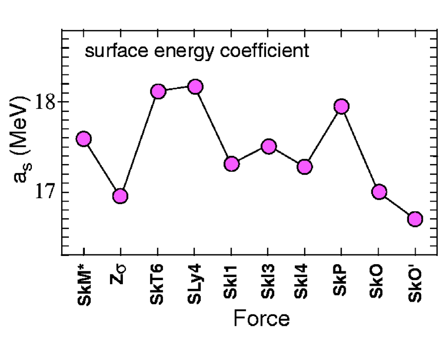
FIG. 1.: The surface energy coefficient as defined in Eq. (21) for the Skyrme parameterizations used in this work.

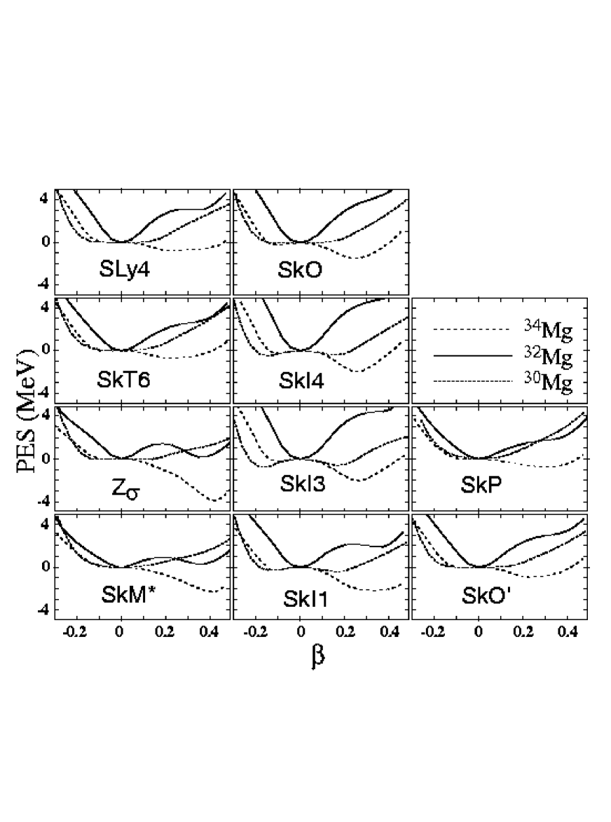
FIG. 2.: Potential energy surfaces for ^30,32,34Mg as functions of quadrupole deformation $\beta$ for the set of Skyrme parameterizations.

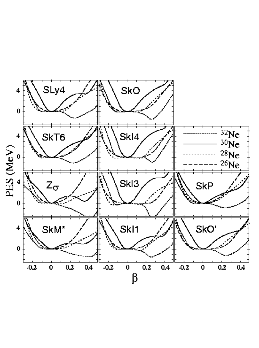
FIG. 3.: Same as in Fig. 2, except for ^26,28,30,32Ne.

FIG. 4.: Same as in Fig. 2, except for ³²Mg and for three different pairing models: volume delta pairing (solid line), no pairing (dotted line), and surface pairing (16) (dashed line).

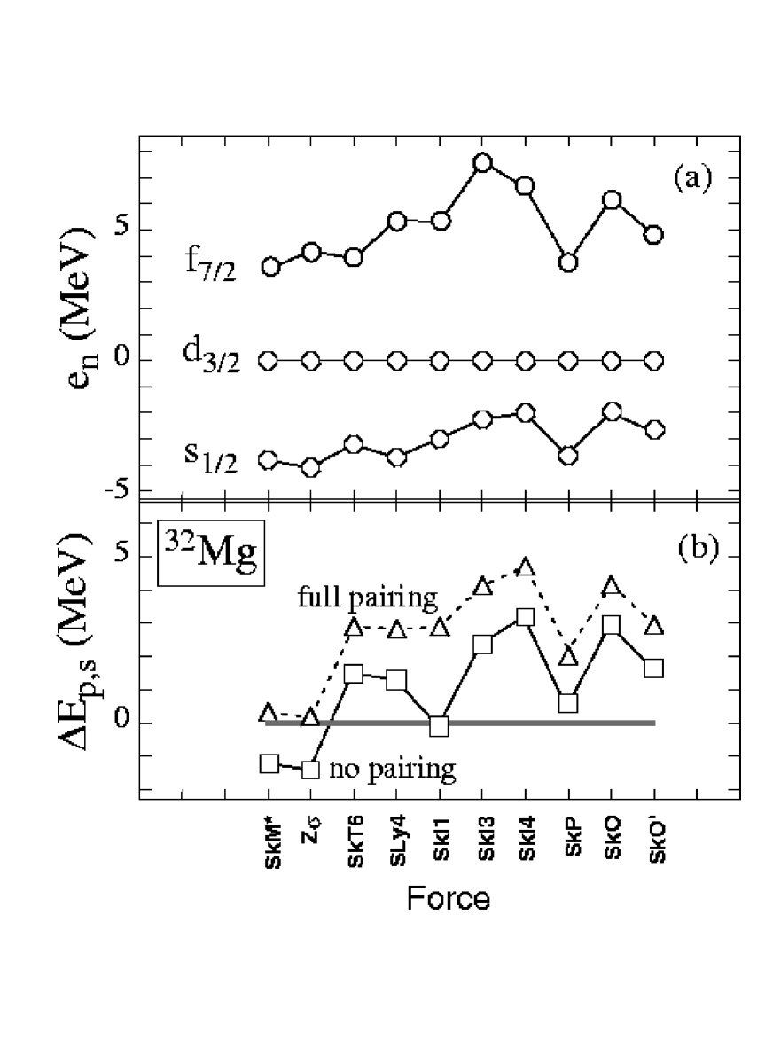
FIG. 5.: Top: Spherical neutron shell structure in ³²Mg calculated in several Skyrme-HF models. The single-particle levels are normalized to the energy of the $d_{3/2}$ shell. Bottom: The prolate-spherical energy difference calculated with (dashed line) and without (solid line) pairing.

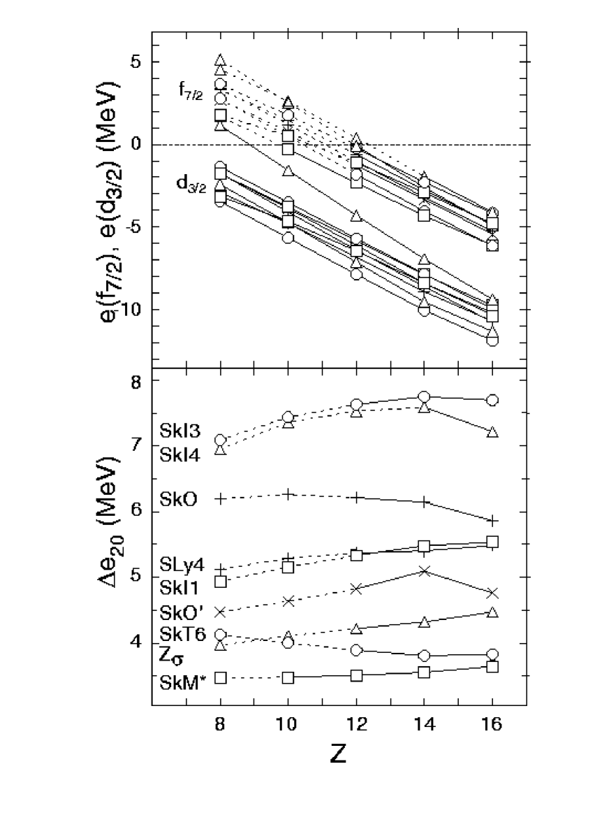
FIG. 6.: Top: Single-neutron $d_{3/2}$ and $f_{7/2}$ energies as functions of $Z$ predicted in several Skyrme-HF models. The positive-energy levels are marked by a dashed line. Bottom: the size of the corresponding single-particle $N$=20 gap, $\Delta e_{20}$.

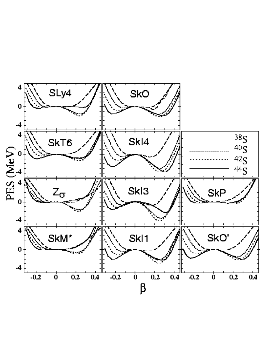
FIG. 7.: Same as in Fig. 2, except for ^38,40,42,44S.

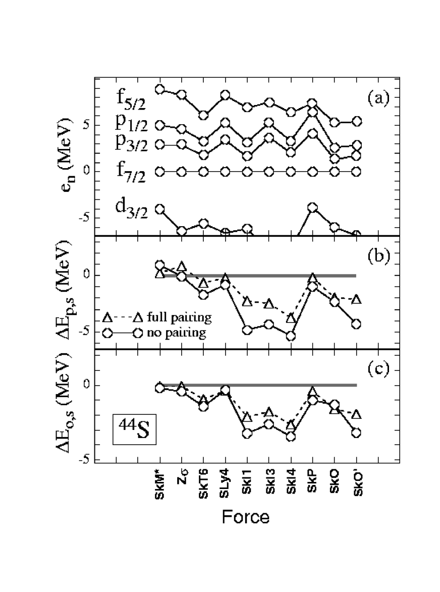
FIG. 8.: Spherical neutron shell structure in ⁴⁴S calculated in several Skyrme-HF models. The single-particle levels are normalized to the energy of the $f_{7/2}$ shell (a); the position of the deformed prolate minimum with respect to the spherical HF state (b); the position of the deformed prolate minimum with respect to the spherical HF state (c).

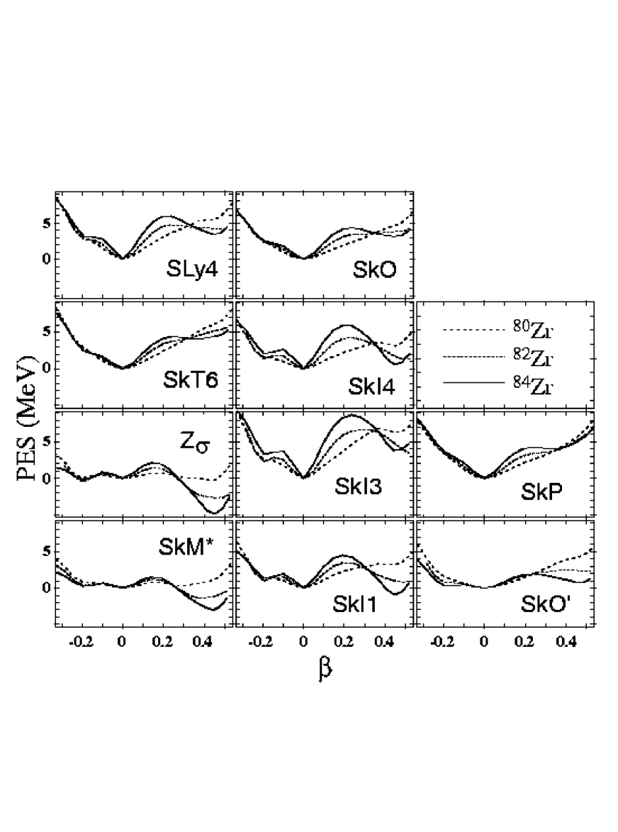
FIG. 9.: Same as in Fig. 2, except for ^80,82,84Zr.

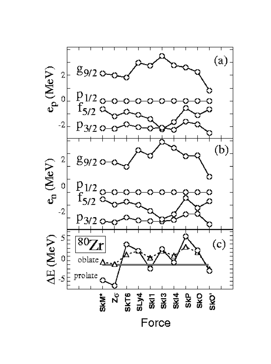
FIG. 10.: Spherical neutron shell structure in ⁸⁰Zr calculated in several Skyrme-HF models. The single-particle levels are normalized to the energy of the $p_{1/2}$ shell (a); spherical proton shell structure (b); the position of the deformed prolate and oblate minima with respect to the spherical HF state (no pairing) (c).

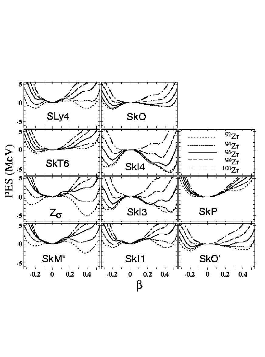
FIG. 11.: Same as in Fig. 2, except for ^{92,94,96,98,100}Zr.

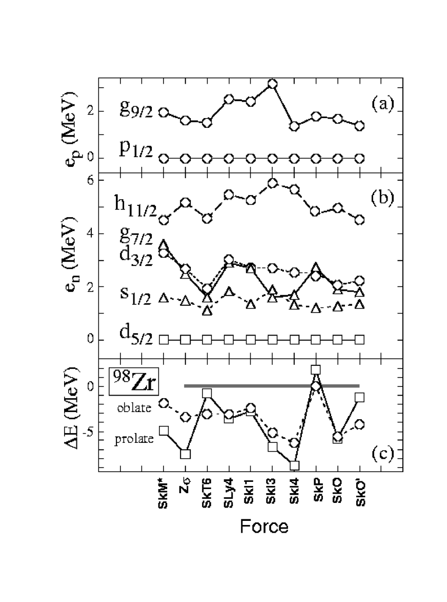
FIG. 12.: Spherical neutron shell structure in ⁹⁸Zr calculated in several Skyrme-HF models. The single-particle levels are normalized to the energy of the $p_{1/2}$ shell (a); spherical proton shell structure, the single-particle levels are normalized to the energy of the $d_{5/2}$ shell (b); the position of the deformed prolate and oblate minima with respect to the spherical HF state (no pairing) (c)

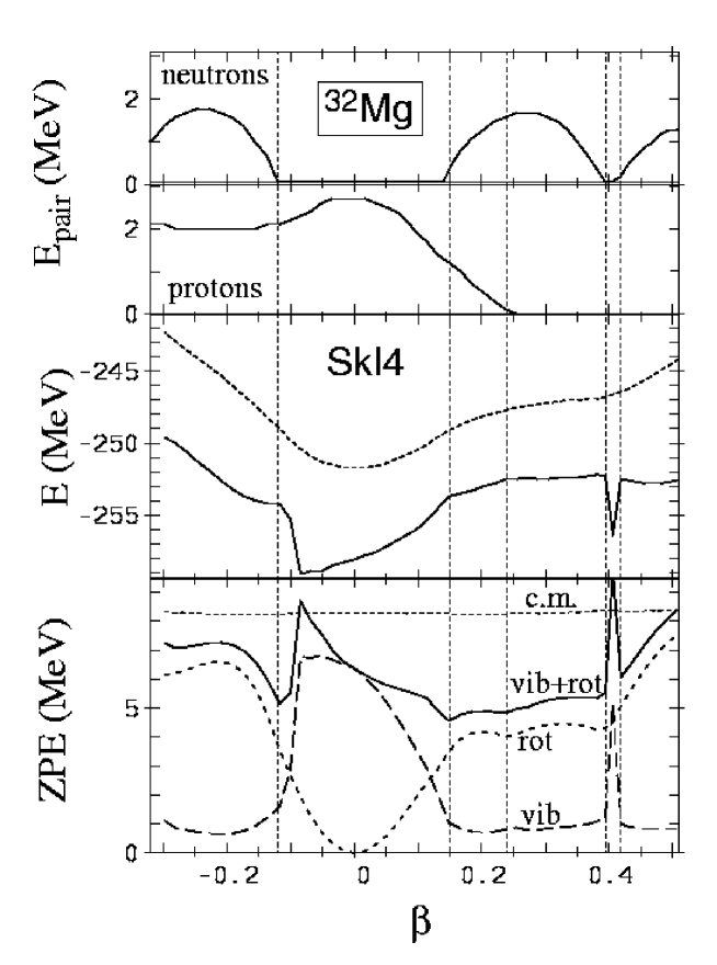
FIG. 13.: The effect of ZPE corrections on the PES of ³²Mg calculated with the SkI4 SKyrme-HF model. Top two: proton and neutron pairing energies. Middle: uncorrected (dashed line) and ZPE-corrected (solid line) PES. Bottom: the various contributions to the ZPE (rotational, dashed line; $\beta$-vibrational, long dashed line; center-of-mass, short dashed line) and the sum of rotational and vibrational corrections, solid line. The vertical lines mark borders of the regions where static pairing (in neutrons or protons) vanishes.

FIG. 14.: Same as in Fig. 13, except for ⁴⁴S.

FIG. 15.: Same as in Fig. 13, except for ⁸⁰Zr.

FIG. 16.: Same as in Fig. 13, except for ⁹⁸Zr.

FIG. 17.: Results of SMMC calculations with the $sdpf$ (left) and $sdpf^{\prime}$ (right) interactions for the neutron-rich Ne and Mg isotopes: Top: $\langle Q_{p}Q_{n}\rangle$; Bottom: $\langle A^{+}A\rangle$ ($J$=0, $T$=1).

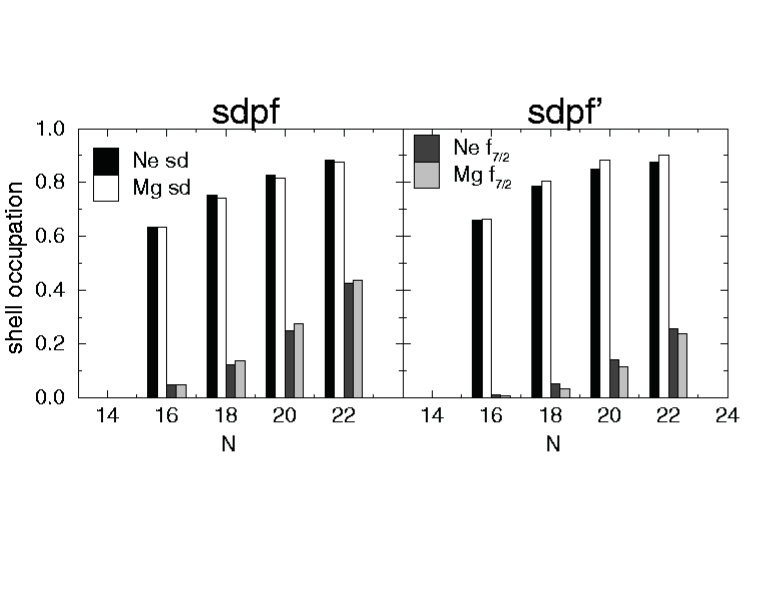
FIG. 18.: Single-neutron shell-model occupations in neutron-rich Ne and Mg isotopes calculated in the SMMC with $sdpf$ (left) and $sdpf^{\prime}$ (right) effective interactions.

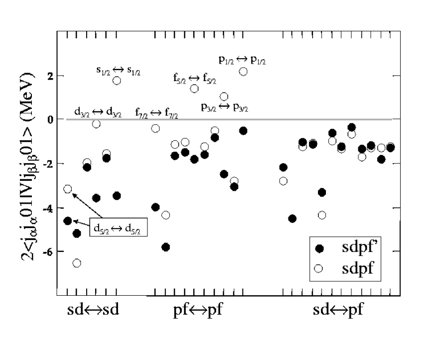
FIG. 19.: $J$=0, $T$=1 matrix elements $\langle j_{\alpha}j_{\alpha}|\hat{V}|j_{\beta}j_{\beta}\rangle$ of the $sdpf$ (open circles) and $sdpf^{\prime}$ (dots) interactions. The diagonal matrix elements ($\alpha$=$\beta$) are indicated. The matrix elements are presented according to the following convention. Assuming that the single-particle orbitals are labeled as: ($d_{5/2}$, $d_{3/2}$, $s_{1/2}$, $f_{f/2}$, $f_{5/2}$, $p_{3/2}$, $p_{1/2}$) $\equiv$ (1, 2, 3, 4 ,5, 6, 7), the first six matrix elements are those within the $sd$ shell [(1,1), (1,2), (1,3), (2,2), (2,3), (3,3)], the next ten are the matrix elements within the $pf$ shell [(4,4),(4,5)…,(7,7)], and the remaining twelve are the cross-shell matrix elements [(1,4), (1,5),…,(3,7)].

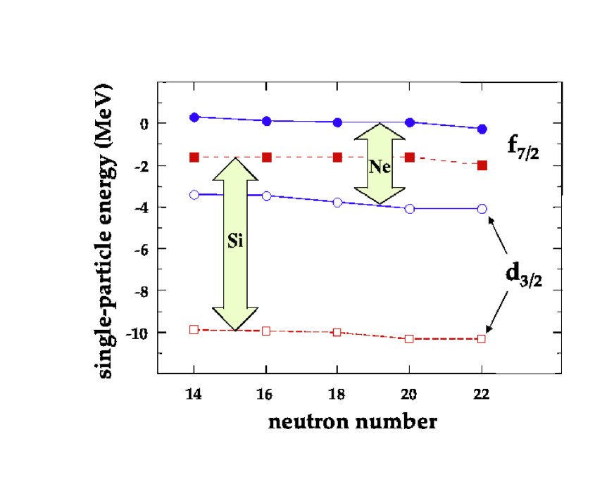
FIG. 20.: Single-particle $1d_{3/2}$ and $1f_{7/2}$ neutron levels (B31) predicted in HFB-SM with the sdpf’ interaction for the Ne and Si isotopes with 14$\leq$$N$$\leq$22. Note that the size of the $N$=20 gap changes very little with $N$.

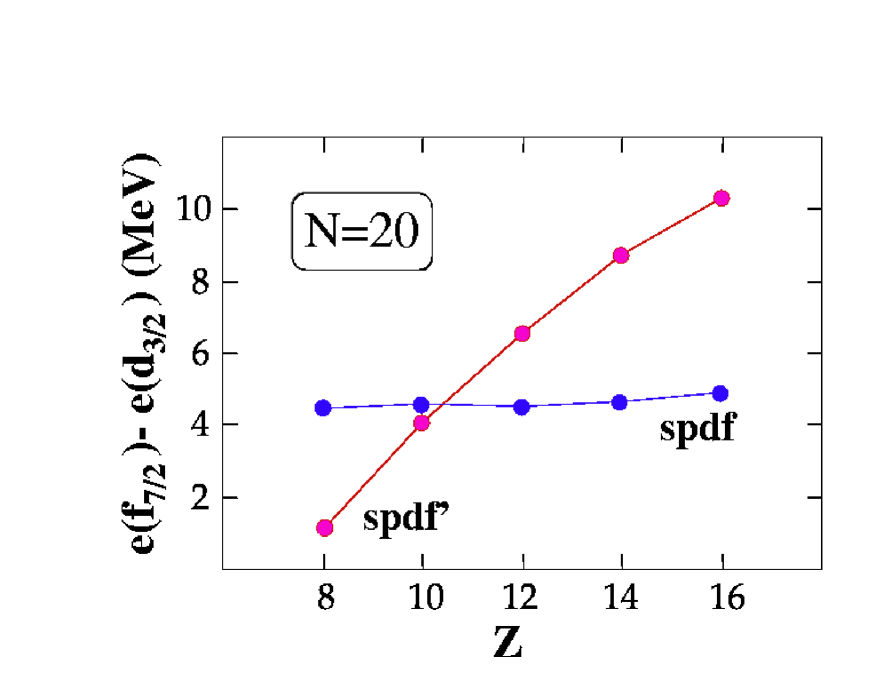
FIG. 21.: Single-particle energy gap at $N$=20, $\Delta e_{20}$, calculated in the HFB-SM with $sdpf$ and $sdpf^{\prime}$ interactions for the $N$=20 isotones of O, Ne, Mg, Si, and S. Note that in $sdpf^{\prime}$ the size of the $N$=20 gap depends dramatically on $Z$.

FIG. 22.: Comparison between the particle-hole matrix elements $V(\alpha,\beta)$, Eq. (B24), of $sdpf$ and $sdpf^{\prime}$. The same convention is used as in Fig. 19. Top: neutron-neutron (proton-proton) matrix elements ($\tau_{\alpha}$=$\tau_{\beta}$). Bottom: proton-neutron matrix elements ($\tau_{\alpha}$=–$\tau_{\beta}$).

FIG. 23.: Correlation energy (41) for the neutron-rich Ne and Mg isotopes. Top: $sdpf$ results. Bottom $sdpf^{\prime}$ results.

FIG. 24.: Size of the $N$=20 gap, $\Delta e_{20}$, obtained from canonical single-particle energies (dashed lines) and the shell-gap parameter (42) obtained from two-neutron separation energies (solid lines) calculated in the HFB approach with Skyrme interactions SkP (dots) and SLy4 (circles).

REFERENCES

- [1] K. Heyde, P. Van Isacker, M. Waroquier, J.L. Wood and R.M. Meyer, Phys. Rep. 102, 291 (1983).
- [2] J.L. Wood, K. Heyde, W. Nazarewicz, M. Huyse, and P. van Duppen, Phys. Rep. 215, 101 (1992).
- [3] P.-G. Reinhard and E.W. Otten, Nucl. Phys. A420, 173 (1984).
- [4] W. Nazarewicz, Nucl. Phys. A574, 27c (1994).
- [5] V.M. Strutinsky, Nucl. Phys. A122, 1 (1968).
- [6] M. Brack, J. Damgård, A.S. Jensen, H.C. Pauli, V.M. Strutinsky and C. Y. Wong, Rev. Mod. Phys. 44, 320 (1972).
- [7] V.M. Strutinsky, Nucl. Phys. A218, 169 (1974).
- [8] M. Brack, C. Guet and H.-B. Håkansson, Phys. Rep. 123, 275 (1985).
- [9] P.H. Heenen, J. Dobaczewski, W. Nazarewicz, P. Bonche, and T.L. Khoo, Phys. Rev. C57, 1719 (1998).
- [10] X. Campi, H. Flocard, A. K. Kerman, and S. Koonin, Nucl. Phys. A251, 193 (1975).
- [11] P.-G. Reinhard, Z. Phys. A285, 93 (1978).
- [12] P.-G. Reinhard and K. Goeke, Rep. Prog. Phys. 50, 1 (1987).
- [13] H. Morinaga, Phys. Rev. 101, 254 (1956).
- [14] K. Heyde, J. Jolie, J. Moreau, J. Ryckebusch, M. Waroquier, P. Van Duppen, M. Huyse, and J. L. Wood, Nucl. Phys. A466, 189 (1987).
- [15] C. Détraz, D. Guillemaud, G. Huber, R. Klapish, M. Langevin, F. Naulin, C. Thibault, L.C. Carraz, and F. Touchard, Phys. Rev. C19, 164 (1979).
- [16] C. Thibault, R. Klapisch, C. Rigaud, A.M. Poskanzer, R. Prieels, L. Lessard, and W. Reisdorf, Phys. Rev. C12 (1975) 644.
- [17] F. Touchard, J. M. Serre, S. Büttenbach, P. Guimbal, R. Klapisch, M. de Saint Simon, C. Thibault, H. T. Duong, P. Juncar, S. Libermen, J. Pinard, and J. L. Vialle, Phys. Rev. C25, 2756 (1982).
- [18] T. Motobayashi, Y. Ikeda, Y. Ando, K. Ieki, M. Inoue, N. Iwasa, T. Kikuchi, M. Kurokawa, S. Moriya, S. Ogawa, H. Murakami, S. Shimoura, Y. Yanagisawa, T. Nakamura, Y. Watanabe, M. Ishihara, T. Teranishi, H. Okuno, and R.F. Casten, Phys. Lett. B 346, 9 (1995).
- [19] M. Barranco and R.J. Lombard, Phys. Lett 78B, 542 (1978).
- [20] P. Möller and J.R. Nix, At. Data Nucl. Data Tables 26, 165 (1981).
- [21] R. Bengtsson, P. Möller, J.R. Nix, J.-y. Zhang, Phys. Scr. 29, 402 (1984).
- [22] A. Watt, M.H. Storm, and R.R. Whitehead, J. Phys. G 7, L145 (1981).
- [23] A. Poves and J. Retamosa, Phys. Lett. 184B, 311 (1987).
- [24] E.K. Warburton, J.A. Becker, and B.A. Brown, Phys. Rev. C41, 1147 (1990).
- [25] N. Fukunishi, T. Otsuka, and T. Sebe, Phys. Lett. B296, 279 (1992).
- [26] A. Poves and J. Retamosa, Nucl. Phys. A571, 221 (1994).
- [27] E. Caurier, F. Nowacki, A. Poves, and J. Retamosa, Phys. Rev. C58, 2033 (1998).
- [28] K. Heyde and J.L. Wood, J. Phys. G17, 135 (1991).
- [29] D. Habs, O. Kester, G. Bollen, L. Liljeby, K.G. Rensfelt, D. Schwalm, R. von Hahn, G. Walter, P. Van Duppen, and the REX-ISOLDE Collaboration, Nucl. Phys. A616, 29c (1997).
- [30] Z. Ren, Z.Y. Zhu, Y.H. Cai, and G. Xu, Phys. Lett. B 380, 241 (1996).
- [31] G.A. Lalazissis, A.R. Farhan, and M.M. Sharma, Nucl. Phys. A628, 221 (1998).
- [32] S.K. Patra and C.R. Praharaj, Phys. Lett. B 273, 13 (1991).
- [33] J. Terasaki, H. Flocard, P.-H. Heenen, and P. Bonche, Nucl. Phys. A621, 706 (1997).
- [34] F. Grümmer, B.Q. Chen, Z.Y. Ma, and S. Krewald, Phys. Lett. B 387, 673 (1996).
- [35] J.F. Berger, J-P. Delaroche, M. Girod, S. Peru, J. Libert, Inst. Phys. Conf. Ser. 132 (IOP, Bristol 1992), p. 487.
- [36] M. Lewitowicz, Yu.E. Penionzhkevich, A.G. Artukh, A.M. Kalinin, V.V. Kamanin, S.M. Lukyanov, Nguyen Hoai Chau, A.C. Mueller, D. Guillemaud-Mueller, R. Anne, D. Bazin, C. Detraz, D. Guerreau, M.G. Saint-Laurent, V. Borrel, J.C. Jacmart, F. Pougheon, A. Richard, and W.D. Schmidt-Ott, Nucl. Phys. A496, 477 (1989).
- [37] O. Sorlin, D. Guillemaud-Mueller, A.C. Mueller, V. Borrel, S. Dogny, F. Pougheon, K.-L. Kratz, H. Gabelmann, B. Pfeiffer, A. Wohr, W. Ziegert, Yu.E. Penionzhkevich, S.M. Lukyanov, V.S. Salamatin, R. Anne, C. Borcea, L.K. Fifield, M. Lewitowicz, M.G. Saint-Laurent, D. Bazin, C. Detraz, F.-K. Thielemann, and W. Hillebrandt, Phys. Rev. C47, 2941 (1993).
- [38] H. Scheit, T. Glasmacher, B.A. Brown, J.A. Brown, P.D. Cottle, P.G. Hansen, R. Harkewicz, M. Hellstrom, R.W. Ibbotson, J.K. Jewell, K.W. Kemper, D.J. Morrissey, M. Steiner, P. Thirolf, and M. Thoennessen, Phys. Rev. Lett. 77, 3967 (1996).
- [39] T. Glasmacher, B.A. Brown, M.J. Chromik, P.D. Cottle, M. Fauerbach, R.W. Ibbotson, K.W. Kemper, D.J. Morrissey, H. Scheit, D.W. Sklenicka, and M. Steiner, Phys. Lett. B 395, 163 (1997).
- [40] H. Savajols et al., Abstracts, ENAM98 (1998), p. A6.
- [41] T.R. Werner, J.A. Sheikh, W. Nazarewicz, M.R. Strayer, A.S. Umar, and M. Misu, Phys. Lett. B333, 303 (1994).
- [42] T.R. Werner, J.A. Sheikh, M. Misu, W. Nazarewicz, J. Rikovska, K. Heeger, A.S. Umar, and M.R. Strayer, Nucl. Phys. A597, 327 (1996).
- [43] D. Hirata, K. Sumiyoshi, B.V. Carlson, H. Toki, and I. Tanihata, Nucl. Phys. A609, 131 (1996).
- [44] G.A. Lalazissis, D. Vretanar, P. Ring, M. Stoitsov, and L. Robledo, nucl-th/9807029.
- [45] J. Retamosa, E. Caurier, F. Nowacki, and A. Poves, Phys. Rev. C55, 1266 (1997).
- [46] W. Nazarewicz, J. Dudek, R. Bengtsson, T. Bengtsson and I. Ragnarsson, Nucl. Phys. A435, 397 (1985).
- [47] C.J. Lister, M. Campbell, A.A. Chishti, W. Gelletly, L. Goettig, R .Moscrop, B.J. Varley, A.N. James, T. Morrison, H.G. Price, J. Simpson, K. Connell, and Ö. Skeppstedt, Phys. Rev. Lett. 59, 1270 (1987).
- [48] A. Petrovici K.W. Schmidt, and A. Faessler, Nucl. Phys. A605, 290 (1996).
- [49] P. Bonche, H. Flocard, P.H. Heenen, S.J. Krieger and M.S. Weiss, Nucl. Phys. A443, 39 (1985).
- [50] P. Bonche, J. Dobaczewski, H. Flocard and P.-H. Heenen, Nucl. Phys. A530, 149 (1991).
- [51] G.A. Lalazissis and M.M. Sharma, Nucl. Phys. A586, 201 (1995).
- [52] E. Kirchuk, P. Federman and S. Pittel, Phys. Rev. C47, 567 (1993).
- [53] J.P. Maharana, Y.K. Gambhir, J.A. Sheikh, and P.Ring, Phys. Rev. C46, R1163 (1992).
- [54] Nuclear Structure of the Zirconium Region, eds. J. Eberth, R.A. Meyer and K. Sistemich (Springer-Verlag, 1988).
- [55] J. Skalski, S. Mizutori, and W. Nazarewicz, Nucl. Phys. A617, 282 (1997).
- [56] W. Nazarewicz, in Contemporary Topics in Nuclear Structure Physics eds. R.F. Casten, A. Frank, M. Moshinsky and S. Pittel (World Scientific, Singapore, 1988) 467.
- [57] J. Dobaczewski, W. Nazarewicz, J. Skalski and T.R. Werner, Phys. Rev. Lett. 60, 2254 (1988).
- [58] T.R. Werner, J. Dobaczewski, M.W. Guidry, W. Nazarewicz, and J.A. Sheikh, Nucl. Phys. A578, 1 (1994).
- [59] P. Quentin and H. Flocard, Annu. Rev. Nucl. Part. Sci. 28, 523 (1978).
- [60] P.-G. Reinhard and H. Flocard, Nucl. Phys. A584, 467 (1995).
- [61] D. Vautherin and D.M. Brink, Phys. Rev. C5, 626 (1972).
- [62] E. Chabanat, Interactions effectives pour des conditions extrêmes d’isospin, Université Claude Bernard Lyon-1, Thesis 1995, LYCEN T 9501, unpublished.
- [63] P.-G. Reinhard et al., in preparation.
- [64] J. Bartel, P. Quentin, M. Brack, C. Guet, and H.B. Håkansson, Nucl. Phys. A386, 79 (1982).
- [65] F. Tondeur, M. Brack, M. Farine, J.M. Pearson, Nucl. Phys. A420, 297 (1984).
- [66] J. Friedrich and P-G.Reinhard, Phys. Rev. C33, 335 (1986).
- [67] J. Dobaczewski, H. Flocard and J. Treiner, Nucl. Phys. A422, 103 (1984).
- [68] M. Bender, P.-G. Reinhard, M.R. Strayer, W. Nazarewicz, in preparation.
- [69] J. Dobaczewski, W. Nazarewicz, T.R. Werner, J.-F. Berger, C.R. Chinn, and J. Dechargé, Phys. Rev. C53, 2809 (1996).
- [70] S.J. Krieger, P. Bonche, H. Flocard, P. Quentin and M.S. Weiss, Nucl. Phys. A517, 275 (1990).
- [71] M. Bender, P.-G. Reinhard, K. Rutz, J.A. Maruhn, preprint, 1998.
- [72] J. Treiner, H. Krivine, O. Bohigas, J. Martorell, Nucl. Phys. A371, 253 (1981).
- [73] J. Fink, V. Blum, P.-G. Reinhard, J. Maruhn, and W. Greiner, Phys. Lett. 218B, 277 (1989).
- [74] A. Góźdź, K. Pomorski, M. Brack, and W. Werner, Nucl. Phys. A442, 26 (1985).
- [75] G.H. Lang, C.W. Johnson, S.E. Koonin, and W.E. Ormand, Phys. Rev. C48, 1518 (1993).
- [76] S.E. Koonin, D.J. Dean, and K. Langanke, Phys. Rep. 278, 1 (1997).
- [77] Y. Alhassid, D.J. Dean, S.E. Koonin, G. Lang, and W.E. Ormand, Phys. Rev. Lett. 72, 613 (1994).
- [78] D.J. Dean, S.E. Koonin, K. Langanke, P.B. Radha, and Y. Alhassid, Phys. Rev. Lett. 74, 2909 (1995).
- [79] D.J. Dean, M.T. Ressell, M. Hjorth-Jensen, S.E. Koonin, K. Langanke, A. Zuker, Phys. Rev. C (1999), in press.
- [80] R. Machleidt, F. Sammarruca, and Y. Song, Phys. Rev. C53, R1483 (1996).
- [81] A.P. Zuker, Nucl. Phys. A576, 65 (1994).
- [82] J. Duflo and A.P. Zuker, submitted to Phys. Rev. Lett.
- [83] B.H. Wildenthal, Progr. Part. Nucl. Phys. 11, 5 (1984).
- [84] T.T.S. Kuo and G.E. Brown, Nucl. Phys. A114, 241 (1968).
- [85] D.J. Millener and D. Kurath, Nucl. Phys. A255, 315 (1975).
- [86] A. Poves and A.P. Zuker, Phys. Rep. 70, 235 (1981).
- [87] Y.M. Engel, D.M. Brink, K. Goeke, S.J. Krieger, and D. Vautherin, Nucl. Phys. A249, 215 (1975).
- [88] P. Hohenberg and W. Kohn, Phys. Rev. 136, B864 (1964).
- [89] M. Levy, Proc. Natl. Acad. Sci. (USA) 76, 6062 (1979).
- [90] F. Azaiez, M. Belleguic, O. Sorlin, S. Leenhardt, M.G. Saint-Laurent, M.J. Lopez, J.C. Angelique, C. Borcea, C. Bourgeois, J.M. Daugat, I. Deloncle, C. Donzaud, J. Duprat, G. de France, A. Gillibert, S. Grevy, D. Guillemaud-Mueller, J. Kiener, M. Lewitowicz, F. Marie, W. Mittig, A.C. Muller, F. De Oliveira, N. Orr, Yu.-E. Penionzhkevich, F. Pougheon, M.G. Porquet, P. Roussel-Chomaz, H. Savajols, W. Shuying, Yu. Sobolev, and J. Winfield, Contrib. Int. Conf. Nuclear Structure’98, Gatlinburg, p. 4 (1998); to be published.