Beta decay of r-process waiting-point nuclei in a self-consistent approach

Abstract

Beta-decay rates for spherical neutron-rich r-process waiting-point nuclei are calculated within a fully self-consistent Quasiparticle Random-Phase Approximation, formulated in the The Hartree-Fock-Bogolyubov canonical single-particle basis. The same Skyrme force is used everywhere in the calculation except in the proton-neutron particle-particle channel, where a finite-range force is consistently employed. In all but the heaviest nuclei, the resulting half-lives are usually shorter by factors of 2 to 5 than those of calculations that ignore the proton-neutron particle-particle interaction. The shorter half-lives alter predictions for the abundance distribution of r-process elements and for the time it takes to synthesize them.

]

I Introduction

The astrophysical r-process [1, 2, 3, 4, 5, 6], which creates about half of all nuclei with $A>70$, proceeds through very neutron-rich and unstable isotopes produced by stellar explosions or other violent events. The ultimate abundance of any stable nuclide depends strongly on the beta-decay half lives of its neutron-rich progenitors. The solar elemental abundance distribution shows peaks near $A$=80, 130, and 195, corresponding to progenitors with closed neutron shells ($N$=50, 82, and 126). These relatively long-lived nuclei not only define the abundance peaks but also restrict the amount of heavier material that is synthesized. Understanding the important features of the r-process therefore requires knowledge of lifetimes of closed-shell semimagic nuclei far from stability. Of course beta decay is only one of the processes that contribute to r-process abundances; neutron capture and photodisintegration also play important roles, as do the temperature, density and initial neutron to seed ratio in the explosive environment. But these other aspects are beyond the scope of this article, which focuses on the crucial question of how to calculate beta decay far from stability. At present, the very neutron-rich nuclei are out of experimental reach, and theory provides the only handle on their decay rates.

Precise theoretical estimates of beta-decay rates are hard to make. Most of the strength associated with the $\beta^{-}$-decay operator ${\mathbf{\sigma}}\tau_{+}$ lies in the Gamow-Teller (GT) resonance, well above decay threshold. The strength that actually contributes to beta decay is the small low-energy tail of the GT distribution. Calculated beta-decay rates can therefore vary over a wide range without coming into conflict with sum rules, which for other processes help reduce theoretical uncertainty. In addition, beta-decay lifetimes depend sensitively on nuclear binding energies, and small errors in calculated $Q_{\beta}$-values can cause large errors in predicted decay rates. These problems are complicated enough to demand a coherent and systematic approach to beta decay. Here we make a first attempt at a completely self-consistent calculation. Our goal, in spite of the difficulties, is a reliable estimate of beta-decay rates in important even-even semimagic nuclei lying on the r-process path.

Special tools are needed to describe transitions to low-lying excited states in weakly bound nuclei. Although large-scale shell model calculations successfully describe the GT strength distribution in medium-mass nuclei close to the valley of beta stability [7, 8], large configuration spaces and difficulties with the continuum [9] make the approach hard to apply along the r-process path. The continuum random phase approximation [10, 11] is often useful, but in very-weakly bound nuclei pairing is important and a quasiparticle random phase approximation (QRPA) based on coordinate-space Hartree-Fock-Bogolyubov (HFB) theory is required. Surprisingly little work has been done along these lines. Much more common are global (in that they attempt to describe all nuclei in the same framework) but non self-consistent calculations [12, 13, 14, 15] that substitute the Strutinsky method + BCS for HFB, approximate the continuum by bound or quasibound orbits, and use a schematic interaction $\kappa({\mathbf{\sigma}}_{1}{\mathbf{\sigma}}_{2})({\mathbf{\tau}}_{1}{\mathbf{\tau}}_{2})$ in the QRPA. The work of Ref. [16], which successfully reproduced the half-lives of the nickel isotopes and of ¹³²Sn in the Tamm-Dancoff approximation, used self-consistent single-particle energies and orbits but retained the traditional schematic residual interaction. But like the global calculations, this work did not include a proton-neutron ($pn$) particle-particle interaction in the QRPA.

Borzov et al. [17, 18] did use a more self-consistent method in restricted regions of the nuclide chart. Their starting point was an energy-density functional optimized for the regions they considered, and a realistic interaction (including a zero-range $pn$ particle-particle component) in the QRPA. Their energy functional was spin-independent, however, and so they did not obtain the residual interaction from the second derivative of the functional, as required if the QRPA is to represent the small amplitude limit of time-dependent HFB (this is what we mean by self-consistency in an HFB + QRPA calculation). Instead they chose a phenomenological spin-dependent residual interaction [17]. In addition, they neglected positive-energy single-particle states in the HFB calculation, though they did include the entire particle-hole continuum in the QRPA. In any event, Borzov et al. [19, 20] have now abandoned attempts at fully self-consistent calculations in favor of the Extended Thomas-Fermi with Strutinsky Integral (ETFSI) approach. No previous papers, in sum, have used the same interaction in the mean-field calculation and the QRPA, and most have neglected the residual $pn$ particle-particle interaction. Neither has any previous work properly included the effects of the low-energy continuum on pairing.

Here we attempt to do better: we use the same interaction in the HFB and QRPA calculations so as to preserve the small-amplitude limit of time-dependent HFB. In the $pn$ particle-particle channel of the QRPA, we use a finite-range interaction to soften the divergences induced by a delta function, but will show that this choice does not spoil self-consistency. By adjusting one parameter, the strength of the $pn$ particle-particle interaction (which we will often refer to as $T$=0 pairing), we reproduce measured decay rates near the closed neutron shells, and then make predictions for rates further from stability. For now we restrict our study to semi-magic nuclei with closed neutron shells and their neighbors; besides being the most important for the r-process these nuclei are conveniently spherical.

Our paper is organized as follows: In Sec. II we review the the general formalism for calculating beta decay, briefly present coordinate-space HFB theory and the QRPA, and then show how to combine them in a self-consistent way. Section III discusses the problem of choosing a good effective interaction. Section IV contains the results of numerical calculations and an r-process simulation, and Sec. V presents conclusions.

II Framework

A Calculation of half-lives

The rate for allowed Gamow-Teller decay of an even-even nucleus is given by

$$\frac{1}{T_{1/2}}=\frac{2\pi}{\ln 2}\frac{g_{A}^{2}}{\hbar}\int\!dE_{e}\sum_{m}|\langle 1^{+}_{m}|\sum_{n}{\mathbf{\sigma}}_{n}\tau^{+}_{n}|0^{+}\rangle|^{2}\;\frac{dn_{m}}{dE_{e}}\ \ ,$$ (1)

where the index $n$ labels particles, $|0^{+}\rangle$ is the initial ground state and the $|1^{+}_{m}\rangle$ are the final states (We use units in which $c$=1.) The sum over $m$ runs over all final 1⁺ states with an excitation energy smaller than the $Q_{\beta^{-}}$ value. We will set the weak axial nucleon coupling constant $g_{A}$ to 1 rather than its actual value of 1.26 to account for the near universal quenching of isovector spin matrix elements [21] in nuclei. The kinematic factor $dn_{m}/dE$ is the density of final ($e^{-},\bar{\nu}_{e}$) states. It can be written as

$$\frac{dn_{m}}{dE_{e}}=\frac{E_{e}\;\sqrt{E_{e}^{2}-m_{e}^{2}}}{2\pi^{3}}\;(E_{i}-E_{1^{+}_{m}}-E_{e})^{2}\;F(Z,E_{e})\ \ ,$$ (2)

where $E_{i}$ is the ground state energy of the even-even initial nucleus with $Z$ protons and $N$ neutrons, $E_{1^{+}_{m}}$ is the energy of the $m$th excited 1⁺ state in the final nucleus with $Z+1$ protons and $N-1$ neutrons, and $F(Z,E_{e})$ corrects the phase-space factor for the nuclear charge and finite nuclear size, both of which affect the electron wave function.

We would like an approximation for $E_{i}-E_{1^{+}_{m}}$ in Eq. (2) that does not require an explicit calculation of the $Q_{\beta^{-}}$ value. To obtain one we express the $Q_{\beta^{-}}$ value in terms of nuclear ground-state binding energies:

$$Q_{\beta^{-}}=\Delta M_{n-H}+B_{\rm g.s.}(Z,N)-B_{\rm g.s.}(Z+1,N-1)$$ (3)

where $\Delta M_{n-H}$=0.78227 MeV is the mass difference between the neutron and the hydrogen atom. The ground-state binding energy of an odd-odd final nucleus, in the independent quasiparticle approximation, is given by

$$B_{\rm g.s.}(Z+1,N-1)\approx B_{\rm g.s.}(Z,N)+\lambda_{p}-\lambda_{n}+E_{2qp,{\rm lowest}}$$ (4)

where $\lambda_{p}$$\equiv$$dE/dZ$ and $\lambda_{n}$$\equiv$$dE/dN$ are the proton and neutron Fermi energies in the initial nucleus ($Z,N$), and $E_{2qp,{\rm lowest}}$ is the energy of the lowest two-quasiparticle excitation (with respect to the initial nucleus) corrected for the residual $pn$ interaction between the valence quasiparticles in the odd-odd system [22]. The excitation energies of the $1^{+}$ states with respect to the final ground state are

$$E^{*}_{1^{+}_{m}}\approx E_{\rm QRPA}-E_{2qp,{\rm lowest}}\quad,$$ (5)

where $E_{\rm QRPA}$ is the QRPA phonon energy (see Sec. II C). It follows from Eqs. (3) and (4) that the energy released in the transition from the ground state of the initial nucleus to a $1^{+}$ state in the final nucleus is

$$E_{i}-E_{1^{+}_{m}} = Q_{\beta_{-}}(Z,N)-E^{*}_{1^{+}_{m}}$$ (6)

$$\approx \lambda_{n}-\lambda_{p}+\Delta M_{n-H}-E_{\rm QRPA}\quad.$$ (7)

This expression allows us to avoid calculating ground-state masses of the final nuclei.

B Skyrme-Hartree-Fock-Bogoliubov Method

Our first-order description of the even-even ground state and quasiparticle excitations is based on a self-consistent mean field. Several schemes are currently used in mean-field calculations for heavy nuclei, among them the non-relativistic HF and HFB methods with the Skyrme interaction [23], the HFB approach with the Gogny force [24], and the relativistic mean-field model [25, 26]. All these provide a parameterized energy functional that describes nuclear properties throughout the chart of nuclides. But in neutron-rich nuclei near the drip-line, where the Fermi energy and pairing potential are close in magnitude, pairing cannot be treated as a small correction to the HF solution. Instead the physics underlying the HF and BCS approaches must be incorporated into a single variational principle, through HFB theory. Our version of HFB is formulated in coordinate space and described in detail in Refs. [27, 28]; here we discuss only the key ingredients needed for calculating beta decay.

Our effective interaction comes from the Skyrme energy-density functional ${\cal E}$. The functional can be divided into two parts:

$${\cal E}={\cal E}_{\rm ph}+{\cal E}_{\rm pair}\quad.$$ (8)

The particle-hole part ${\cal E}_{\rm ph}$ depends primarily on the density matrix $\rho_{q}({\mathbf{r}}\sigma,{\mathbf{r}}^{\prime}\sigma^{\prime})$, while the pairing (particle-particle) part ${\cal E}_{\rm pair}$ depends primarily on the pairing density matrix $\chi_{q}({\mathbf{r}}\sigma,{\mathbf{r}}^{\prime}\sigma^{\prime})$ (the index $q$ denotes protons or neutrons). The coupling between $\rho$ and $\chi$ comes from the density-dependent terms of the Skyrme and/or pairing interaction. Because the nuclei we consider are so neutron-rich, we shall neglect $pn$ pairing in the HFB ground state (see Sec. III); as a result our HFB wave function will be a product of proton and neutron wave functions, and matrices of $\rho$ and $\chi$ will be block diagonal in $q$. Expressions defining the Skyrme and pairing energy functionals have been presented many times (see e.g. Refs. [29, 30, 31, 32]), and so are only briefly discussed here in Secs. III A and III B.

The particle-hole, $h_{q}({\mathbf{r}}\sigma,{\mathbf{r}}^{\prime}\sigma^{\prime})$, and particle-particle, $\Delta_{q}({\mathbf{r}}\sigma,{\mathbf{r}}^{\prime}\sigma^{\prime})$, mean fields are defined as the first derivatives of the energy functional with respect to the corresponding densities:

$$h_{q}({\mathbf{r}}\sigma,{\mathbf{r}}^{\prime}\sigma^{\prime}) = \frac{\delta{\cal E}}{\delta\rho_{q}({\mathbf{r}}^{\prime}\sigma^{\prime},{\mathbf{r}}\sigma)}\quad,$$ (9)

$$\Delta_{q}({\mathbf{r}}\sigma,{\mathbf{r}}^{\prime}\sigma^{\prime}) = \frac{\delta{\cal E}}{\delta\chi_{q}({\mathbf{r}}^{\prime}\sigma^{\prime},{\mathbf{r}}\sigma)}\quad.$$ (10)

The residual interactions that enter the QRPA equations (discussed in Sec. II C) are the corresponding second derivatives of the energy functional. Rearrangement terms, which result from the density dependence of the energy functional are therefore included in the both the HFB and the QRPA.

Variation of the energy functional (8) with respect to the densities leads to the coordinate-space HFB equations for protons and neutrons [27],

$$\int \!d^{3}r^{\prime} \sum_{\sigma^{\prime}}\left(\!\begin{array}[]{cc}h_{q}({\mathbf{r}}\sigma,{\mathbf{r}}^{\prime}\sigma^{\prime})&\Delta_{q}({\mathbf{r}}\sigma,{\mathbf{r}}^{\prime}\sigma^{\prime})\\ \Delta_{q}({\mathbf{r}}\sigma,{\mathbf{r}}^{\prime}\sigma^{\prime})&-h_{q}({\mathbf{r}}\sigma,{\mathbf{r}}^{\prime}\sigma^{\prime})\end{array}\!\right)\!\left(\!\begin{array}[]{c}\phi_{1}(\alpha,{\mathbf{r}}^{\prime}\sigma^{\prime})\\ \phi_{2}(\alpha,{\mathbf{r}}^{\prime}\sigma^{\prime})\end{array}\!\right)$$ (15)

$$= \left(\begin{array}[]{cc}E_{\alpha}+\lambda_{q}&0\\ 0&E_{\alpha}-\lambda_{q}\end{array}\right)\left(\begin{array}[]{c}\phi_{1}(\alpha,{\mathbf{r}}\sigma)\\ \phi_{2}(\alpha,{\mathbf{r}}\sigma)\end{array}\right),$$ (20)

where $\alpha$ enumerates the HFB quasiparticle eigenstates. The two-component quasiparticle wave functions $\phi_{1}(\alpha,{\mathbf{r}}^{\prime}\sigma^{\prime})$ and $\phi_{2}(\alpha,{\mathbf{r}}^{\prime}\sigma^{\prime})$ self-consistently define the densities:

$$\rho_{q}({\mathbf{r}}\sigma,{\mathbf{r}}^{\prime}\sigma^{\prime}) = \sum_{\alpha\in q}\phi_{2}(\alpha,{\mathbf{r}},\sigma)\;\phi_{2}^{*}(\alpha,{\mathbf{r}}^{\prime},\sigma^{\prime})\quad,$$ (21)

$$\chi_{q}({\mathbf{r}}\sigma,{\mathbf{r}}^{\prime}\sigma^{\prime}) = \sum_{\alpha\in q}\phi_{1}(\alpha,{\mathbf{r}},\sigma)\;\phi_{2}^{*}(\alpha,{\mathbf{r}}^{\prime},\sigma^{\prime})\quad,$$ (22)

The Lagrange multipliers $\lambda_{q}$ — the Fermi energies of the neutrons and protons — are fixed by the particle-number conditions

$$N_{q}=\int\!d^{3}r\sum_{\sigma=\pm}\rho_{q}({\mathbf{r}}\sigma,{\mathbf{r}}\sigma)\quad.$$ (23)

By working directly in the coordinate space we are able to properly include unbound states, which, as we have remarked, become important near the neutron drip line. A particular virtue of our approach is the accurate representation of the canonical single-particle basis, consisting of eigenstates $\psi_{q\mu}(\mathchoice{{\hbox{\boldmath$\displaystyle r$}}}{{\hbox{\boldmath$\textstyle r$}}}{{\hbox{\boldmath$\scriptstyle r$}}}{{\hbox{\boldmath$\scriptscriptstyle r$}}}\sigma)$ of the density matrix:

$$\int{d}^{3}{r}^{\prime}\sum_{\sigma^{\prime}}\rho_{q}(\mathchoice{{\hbox{\boldmath$\displaystyle r$}}}{{\hbox{\boldmath$\textstyle r$}}}{{\hbox{\boldmath$\scriptstyle r$}}}{{\hbox{\boldmath$\scriptscriptstyle r$}}}\sigma,\mathchoice{{\hbox{\boldmath$\displaystyle r$}}}{{\hbox{\boldmath$\textstyle r$}}}{{\hbox{\boldmath$\scriptstyle r$}}}{{\hbox{\boldmath$\scriptscriptstyle r$}}}^{\prime}\sigma^{\prime})\psi_{q\mu}(\mathchoice{{\hbox{\boldmath$\displaystyle r$}}}{{\hbox{\boldmath$\textstyle r$}}}{{\hbox{\boldmath$\scriptstyle r$}}}{{\hbox{\boldmath$\scriptscriptstyle r$}}}^{\prime}\sigma^{\prime})=v^{2}_{q\mu}\psi_{q\mu}(\mathchoice{{\hbox{\boldmath$\displaystyle r$}}}{{\hbox{\boldmath$\textstyle r$}}}{{\hbox{\boldmath$\scriptstyle r$}}}{{\hbox{\boldmath$\scriptscriptstyle r$}}}\sigma).$$ (24)

Canonical states form an infinite, discrete, and complete set of localized wave functions [27, 28]; they describe both the bound states and the positive-energy single-particle continuum. The canonical basis is well defined for all particle-bound nuclei, no matter how close they are to the drip line. We use it in the next section to formulate the QRPA.

C Proton-neutron QRPA

Although one can derive coordinate-space QRPA equations for the generalized density matrix [10, 17, 18], here we stick with the older representation in terms of a discrete single-particle basis. The canonical HFB basis is ideal for this purpose because it simplifies the HFB equations, so that HFB + QRPA can be formulated in complete parallel with BCS + QRPA (described, e.g., in Ref. [33]). The $pn$ QRPA equations take the form:

$$\left(\begin{array}[]{rr}A&B\\ -B&-A\end{array}\right)\left(\begin{array}[]{c}X\\ Y\end{array}\right)=E_{\rm QRPA}\left(\begin{array}[]{c}X\\ Y\end{array}\right)\quad,$$ (25)

with matrices $A$ and $B$ defined as

$$A_{pn,p^{\prime}n^{\prime}} = E_{p,p^{\prime}}\;\delta_{n,n^{\prime}}+E_{n,n^{\prime}}\;\delta_{p,p^{\prime}}$$ (28)

$$+\tilde{V}_{pn,p^{\prime}n^{\prime}}(u_{p}v_{n}u_{p^{\prime}}v_{n^{\prime}}+v_{p}u_{n}v_{p^{\prime}}u_{n^{\prime}})$$

$$+V_{pn,p^{\prime}n^{\prime}}(u_{p}u_{n}u_{p^{\prime}}u_{n^{\prime}}+v_{p}v_{n}v_{p^{\prime}}v_{n^{\prime}})$$

and

$$B_{pn,p^{\prime}n^{\prime}} = \tilde{V}_{pn,p^{\prime}n^{\prime}}(v_{p}u_{n}u_{p^{\prime}}v_{n^{\prime}}+u_{p}v_{n}v_{p^{\prime}}u_{n^{\prime}}$$ (30)

$$-V_{pn,p^{\prime}n^{\prime}}(u_{p}u_{n}v_{p^{\prime}}v_{n^{\prime}}+v_{p}v_{n}u_{p^{\prime}}u_{n^{\prime}})\quad.$$

Here $p$, $p^{\prime}$, and $n$, $n^{\prime}$ denote proton and neutron quasiparticle canonical states, $\tilde{V}$ is the $pn$ particle-hole interaction in the $1^{+}$ channel, obtained from the second derivative of energy functional ${\cal E}$ with respect to the proton and neutron densities, and $V$ is the corresponding particle-particle interaction, obtained from the second derivative with respect to the pairing densities. The $X$’s and $Y$’s are the amplitudes for exciting two-quasiparticle and two-quasihole states from the correlated vacuum. The occupation amplitudes $v_{i}$ are the eigenvalues of the density matrix (24). Since the canonical HFB basis does not diagonalize the HFB Hamiltonian (20), the one-quasiparticle terms in the Eq. (28) have off-diagonal matrix elements $E_{i,j}$. The presence of these terms is the only formal difference between our QRPA equations and those based on the BCS approximation. The localized canonical wave functions, however, are more realistic than the single-quasiparticle states used to mock up the continuum in the BCS approximation.

To actually solve the matrix QRPA equations (25) we have to truncate the canonical basis. The diagonal matrix elements of the one-quasiparticle Hamiltonian provide a convenient measure of excitation, and we include only those canonical states for which these matrix elements are less than a cut-off value. (For the choice of the cut-off energy, see Sec. III.) Occupation probabilities of canonical states usually decrease much faster with excitation energy than in the BCS approximation [28], allowing us to work with matrices of manageable size.

III Interactions

Different channels of the effective interaction have different effects on the beta-strength function. Roughly speaking, the like-particle and $pn$ particle-hole interactions determine the single-particle spectrum. The like-particle pairing interaction smears the Fermi surface and changes the elementary excitations from particles to quasiparticles. Without further many-body correlations, the GT resonance is not collective and too much of the beta strength is located at low energies. The $pn$ particle-hole force, treated in the QRPA, solves the problem by pushing GT strength up and into the resonance, leaving the low-lying spectrum depleted. This depletion is so great, however, that the resulting lifetimes can become too long; the half-lives of Refs [12], for example, usually exceed measured half-lives. The $pn$ particle-particle force cures this problem by pulling some strength back down. Interestingly, this part of the force is also necessary to describe $\beta^{+}$ decay in proton-rich nuclei, but there it decreases the low-lying strength.

To be consistent, one should use a single interaction in all channels and in every step of calculation. This means, for example, that the same $pn$ particle-hole energy functional that determines single-particle properties in the HFB calculation must also be used in the QRPA. The same is true for the pairing (particle-particle) forces, both in the like-particle and $pn$ channels. The constraint is not as tight as in the particle-hole channel, however, because the proton and neutron Fermi surfaces are so far apart in neutron-rich nuclei that $pn$ pairing correlations are neglibigle in the HFB. Furthermore, to the extent that the $T$=1 pairing force can be approximated by a delta function, it does not affect the $J^{\pi}$=1⁺ states obtained in the QRPA. Even with a finite range force, the effects are negligible. The $pn$ component of the $T$=1 pairing/particle-particle interaction can therefore be neglected everywhere. In addition, one is free to choose the $T$=0 pairing component solely on the basis of its effects in the QRPA, since it has no like-particle component and does nothing at the mean field level unless $N$$\approx$$Z$.

For these reasons we organize the discussion in this section as follows: First we describe the particle-hole interaction in detail; it largely determines both single-particle properties and the collectivity of the GT resonance. We then briefly discuss the like-particle pairing force, which plays a role only in the HFB calculation. Finally, we describe the $pn$ ($T$=0) pairing interaction. This last ingredient appears only in the QRPA but, as mentioned already, is crucial for reducing calculated lifetimes to values that are consistent with experiment.

A The particle-hole interaction

The $pn$ particle-hole interaction is responsible for the main features of the GT distribution. For our calculations to make sense, we need to find an interaction that reproduces the distribution reasonably, at both high and low energies. Before doing this, we have to discuss the general form of the particle-hole interaction in the Skyrme framework.

For even-even nuclei, the particle-hole Skyrme energy functional of Eq. (8) can be written as

$${\cal E}_{\rm ph}={\cal E}_{\rm kin}+{\cal E}_{\rm Sk}+{\cal E}_{\rm C}\quad,$$ (31)

i.e. as the sum of a kinetic-energy functional ${\cal E}_{\rm kin}$, an effective strong-interaction functional ${\cal E}_{\rm Sk}$, and a Coulomb functional ${\cal E}_{\rm C}$. The functionals are the spatial integrals of the corresponding local energy densities ${\cal H}$,

$${\cal E}[\rho,\tau,{\bf J}]=\int\!{\rm d}^{3}r\;{\cal H}[\rho({\bf r}),\tau({\bf r}),{\bf J}({\bf r})]\quad.$$ (32)

The kinetic-energy and Coulomb energy densities are given by

$${\cal H}_{\rm kin} = \frac{\hbar^{2}}{2m}\;\tau\quad,$$ (33)

$${\cal H}_{\rm C} = \frac{e^{2}}{2}\int\!{\rm d}^{3}r^{\prime}\frac{\rho_{\rm p}({\mathbf{r}})\rho_{\rm p}({\mathbf{r}}^{\prime})}{|{\mathbf{r}}-{\mathbf{r}}^{\prime}|}-\frac{3e^{2}}{4}\left(\frac{3}{\pi}\right)^{1/3}\!\!\rho_{\rm p}^{4/3}\quad.$$ (34)

The Skyrme energy density can be split into pieces ${\cal H}_{\rm Sk}^{\rm even}$ and ${\cal H}_{\rm Sk}^{\rm odd}$ that are bilinear in time-even and time-odd densities, respectively [30, 34]. Only ${\cal H}_{\rm Sk}^{\rm even}$ affects the ground-state properties of even-even nuclei; it can be written as

$${\cal H}_{\rm Sk}^{\rm even} = \frac{b_{0}}{2}\rho^{2}+b_{1}\rho\tau-\frac{b_{2}}{2}\rho\Delta\rho+\frac{b_{3}}{3}\rho^{\alpha+2}-b_{4}\rho{\mathbf{\nabla}}\cdot{\mathbf{J}}$$ (38)

$$-\sum_{q}\left[\frac{b^{\prime}_{0}}{2}\rho_{q}^{2}+b^{\prime}_{1}\rho_{q}\tau_{q}-\frac{b^{\prime}_{2}}{2}\rho_{q}\Delta\rho_{q}\right.$$

$$+\left.\frac{b^{\prime}_{3}}{3}\rho^{\alpha}\rho_{q}^{2}+b_{4}^{\prime}\rho_{q}{\mathbf{\nabla}}\cdot{\mathbf{J}}_{q}\right]$$

$$-\frac{1}{2}\Big{[}c_{1}{\mathbf{J}}^{2}-c_{1}^{\prime}\sum_{q}{\mathbf{J}}_{q}^{2}\Big{]}\quad.$$

The energy densities depend on the local matter density $\rho_{q}$, the kinetic density $\tau_{q}$, and the spin-orbit current ${\mathbf{J}}_{q}$. Densities without a $q$ index are total (isoscalar) densities, e.g. $\rho_{0}=\rho_{p}+\rho_{n}$. The parameters $b_{i}$, $b_{i}^{\prime}$, $c_{1}$, and $c_{1}^{\prime}$ are the time-even coupling constants of the Skyrme functional. The parameters all play different roles; the terms with $b_{3}$ and $b_{3}^{\prime}$, for example, determine the density-dependent parts of the interaction, and the $b_{4}$, $b_{4}^{\prime}$ and $c_{1}$, $c_{1}^{\prime}$ terms define the spin-orbit interaction. All the parameters are fit to a few key nuclear-structure data, e.g. total binding energies, charge radii, and surface thicknesses of nuclei in the valley of stability, and they generally reproduce ground-state properties of nuclei between ¹⁶O and the heaviest elements [35, 36].

The energy density ${\cal H}_{\rm Sk}^{\rm odd}$, the detailed form of which can be found in Ref. [34], involves time-odd quantities: the momentum density, spin density, and vector part of kinetic-energy density. The time-odd terms contribute to the energy of polarized states, i.e. those with nonzero angular momentum, including the $1^{+}$ states populated by beta decay. As a consequence, the distribution of GT strength depends primarily on this time-odd part of the energy density. Although most of the coefficients in ${\cal H}_{\rm Sk}^{\rm odd}$ are in principle independent parameters, they are fixed by the values of the parameters in ${\cal H}_{\rm Sk}^{\rm even}$ in the usual Skyrme ansatz [34]. The restriction is not in the spirit of the local density approximation [37, 38], but has been made implicitly in almost all prior work. The predictions of most existing Skyrme forces for excited states in odd-odd nuclei are therefore completely determined by fits of ${\cal H}_{\rm Sk}^{\rm even}$ to properties of even-even ground states. Not surprisingly, we find the GT spectra predicted by most of these forces to be well off the mark.

Clearly, the proper approach to beta decay in the Skyrme framework is to fit coefficients in ${\cal H}_{\rm Sk}^{\rm odd}$ to properties of nuclear states with non-zero angular momentum. That task is not so easy, however. Excited states take more computer time to explore than ground states because they require methods beyond mean-field theory (such as the QRPA). Furthermore, ${\cal H}_{\rm Sk}^{\rm odd}$ contains many parameters, and fixing them all would be a major undertaking. For these reasons, we have chosen here to use the relations between time-even and time-odd densities imposed by the the traditional Skyrme-force ansatz, in spite of the drawbacks. (The ansatz, incidentally, relates the $b_{i}$, $b_{i}^{\prime}$, $c_{1}$, and $c_{1}^{\prime}$ of Eq. (38) to the usual Skyrme-force parameters $t_{i}$ and $x_{i}$, as spelled out in Ref. [35].) We will explore the effects of independent time-odd densities in a future publication.

TABLE I.: Properties of symmetric nuclear matter at saturation density $\rho_{0}$ predicted by representative Skyrme interactions. $E/A$ is the energy per nucleon, $m^{*}/m$ the effective mass, $K_{\infty}$ the incompressibility, and $a_{\text{sym}}$ the asymmetry coefficient. The remaining quantities are the Landau-Migdal parameters $f_{0},f_{0}^{\prime},g_{0}$, and $g_{0}^{\prime}$ [39]; $g_{0}^{\prime}$ controls the effective interaction in the spin-isospin channel. The empirical values were taken from Ref. [43]

Force	$\rho_{0}$	$E/A$	$m^{*}/m$	$K_{\infty}$	$a_{\text{sym}}$	$f_{0}$	$f_{0}^{\prime}$	$g_{0}{}{}$	$g_{0}^{\prime}{}{}$
	${[{\rm fm}^{-3}]}$	${[{\rm MeV}]}$			${[{\rm MeV}]}$
SGII	$0.158$	$-15.58$	$0.786$	$214$	$26.8$	$-0.233$	$0.728$	$0.622$	$0.934$
SkM*	$0.160$	$-15.75$	$0.789$	$216$	$30.0$	$-0.229$	$0.926$	$0.325$	$0.937$
SkP	$0.162$	$-15.93$	$1.000$	$201$	$30.0$	$-0.102$	$1.417$	$-0.229$	$0.062$
SLy4	$0.160$	$-15.97$	$0.694$	$230$	$32.0$	$-0.276$	$0.813$	$1.385$	$0.901$
SLy5	$0.161$	$-15.98$	$0.698$	$230$	$32.0$	$-0.276$	$0.814$	$1.137$	$-0.152$
SLy6	$0.159$	$-15.92$	$0.690$	$230$	$32.0$	$-0.280$	$0.803$	$1.408$	$0.899$
SkI4	$0.160$	$-15.92$	$0.650$	$248$	$29.5$	$-0.273$	$0.559$	$1.768$	$0.881$
SkO’	$0.160$	$-15.75$	$0.896$	$222$	$32.0$	$-0.097$	$1.328$	$-1.612$	$0.792$
Empirical						$0\pm 0.3$	$\sim 1.6$	$\sim 0.4$	$\sim 1.80$

Even with constraints on ${\cal H}_{\rm Sk}^{\rm odd}$, it is difficult to include excited-state properties in the data set used to fit ${\cal H}_{\rm Sk}^{\rm even}$. Instead we follow the approach advocated in Ref. [39] and compare the effective strength of our spin- and isospin-flip interaction in nuclear matter with phenomenological values or predictions of realistic calculations. In nuclear matter the interaction strength in the GT channel is sensitive to a single combination of the Skyrme parameters, the Landau-Migdal parameter $g_{0}^{\prime}$ [39]:

$$g_{0}^{\prime} = -N_{0}\Big{[}{\textstyle\frac{1}{3}}\Big{(}b_{0}+{\textstyle\frac{1}{2}}b_{0}^{\prime}\Big{)}+{\textstyle\frac{2}{9}}\Big{(}b_{3}+{\textstyle\frac{1}{2}}b_{3}^{\prime}\Big{)}\,\rho^{\alpha}+c_{1}^{\prime}k_{F}^{2}\Big{]}~{},$$ (39)

where we have used the normalization factor $N_{0}$ = $2k_{F}m^{*}/(\pi^{2}\hbar^{2})$, with the Fermi momentum defined as $k_{F}$ = $(3\pi^{2}\,\rho/2)^{1/3}$. Table I shows predictions of representative Skyrme interactions – SGII [39]; SkM^∗ [40]; SkP [27]; SLy4, SLy5 [41]; SkI4 [35]; and SkO’ [42] – for properties of symmetric nuclear matter at saturation density. While all the forces give about the same saturation density $\rho_{0}$, energy per nucleon $E/A$, and incompressibility $K_{\infty}$, small but noticeable differences appear in the effective mass $m^{*}$ and asymmetry coefficient $K_{\infty}$. The Landau parameter $f_{0}$ is a combination of $\rho_{0}$, $m^{\ast}$ and $K_{\infty}$, and $f_{0}^{\prime}$ is related to $\rho_{0}$ and $m^{\ast}$; it is therefore not surprising that most forces predict similar values for the time-even quantities $f_{0}$ and $f_{0}^{\prime}$, and that those values are close the empirical ones [43]. But the parameters $g_{0}$ and $g_{0}^{\prime}$, which act in time-odd channels, reflect spin-dependent components that are not constrained by standard fits. As a result their values scatter within a wide range: $-1.6\lesssim g_{0}\lesssim+1.8$ and $-0.2\lesssim g_{0}^{\prime}\lesssim+1$. Furthermore, two otherwise very similar forces can give quite different values for these parameters. The interactions SLy4 and SLy5, for example, are identical for one small detail, the treatment of the ${\mathbf{J}}^{2}$ term during the fit. But despite the close agreement for most nuclear-matter parameters, the differences in both $g_{0}$ and $g_{0}^{\prime}$ between the two are significant.

We remarked above that predictions of existing Skyrme forces for GT distributions usually are not good. This fact is reflected in Table I by the values of $g_{0}^{\prime}$, all of which are much smaller than the empirical value $g_{0}^{\prime}({\rm expt})\approx 1.8$ [43]. In fact, we are not aware of a single Skyrme interaction that gives $g_{0}^{\prime}$ close to the empirical value and at the same time does an acceptable job with global nuclear properties and single-particle shell structure. State-of-the-art Skyrme forces tend to yield a $g_{0}^{\prime}$ of about 0.9, a value too small by a factor two. An important related point: the value $g_{0}^{\prime}$=0.503 reported for SGII in Ref. [39] does not correspond to the consistent application of any Skyrme force. The authors left out the last term (in brackets) in Eq. (38) when fitting the parameters of their force, but included its effects in their calculation of $g_{0}^{\prime}$ (and in their RPA calculations). To be consistent with their mean-field interaction, they should have omitted the term proportional to $k_{F}^{2}$ in Eq. (39). Doing so gives $g_{0}^{\prime}$=$0.93$, the value in Table I. We will elaborate on this remark in a future paper. For now, what’s important is that even calculated properly the value of $g_{0}^{\prime}$ associated with this interaction, which was designed explicitly for GT resonances, is far too small.

Of course $g_{0}^{\prime}$ in symmetric nuclear matter at saturation density does not directly measure the strength of spin- and isospin-flip interactions in a finite nucleus. All effects due to the nuclear surface, finite nuclear volume, and excess neutrons disappear in nuclear matter. Moreover, the GT distribution depends strongly on the single-particle spectrum as well as the residual interaction. Nonetheless, the parameter $g_{0}^{\prime}$ summarizes the gross features of the distribution. This is illustrated in Figs. 1 and 2, which display the summed GT strength calculated for ⁹⁰Zr and ¹²⁸Cd. Here we use three Skyrme forces with different values of Landau-Migdal parameter: SkO’ ($g_{0}^{\prime}$=0.792), SkP ($g_{0}^{\prime}$=0.062), and SLy5 ($g_{0}^{\prime}$=–0.152). In general both the energy of the GT resonance and the strength in it increase with $g_{0}^{\prime}$; they are smallest for SLy5 and largest for SkO’. Forces with small values of $g_{0}^{\prime}$ fail to concentrate enough strength in the resonance, leaving too much at low energy.

Although none of the interactions have large enough $g_{0}^{\prime}$ when used self-consistently, some are better than others. Having opted for now not to increase $g_{0}^{\prime}$ by using energy functionals in which ${\cal H}^{\rm even}_{\rm Sk}$ and ${\cal H}^{\rm odd}_{\rm Sk}$ decoupled, we decided to use SkO’ [42], which has one of the larger values in Table I. The SkO’ energy functional is more general than the original Skyrme functionals in the spin orbit channel; the extra generality manifests itself as a difference in the values of $b_{4}$ and $b_{4}^{\prime}$ [35]. Without this extended interaction it seems to be impossible to obtain a consistent description of spin-orbit splittings and other global observables unless the last term in brackets in Eq. (38) is neglected [44]. The extension remedies the problem quite nicely, and in spite of the low value of $g_{0}^{\prime}$, SkO’ reproduces GT spectra [45] measured in charge-exchange reactions fairly well. The predicted resonances, though usually a little too low in energy, contain about the correct fraction of the strength.

FIG. 1.: Summed GT strength up to 20 MeV as a function of excitation energy for the closed-shell nucleus ⁹⁰Zr, calculated with the SkO’, SLy5, and SkP Skyrme forces. We also plot the measured strength reported in Ref. [59] The calculated strength, as is customary, is multiplied by $(1/1.26)^{2}$; the quenching corresponds to setting $g_{A}$ to 1.0 in our calculations of beta decay.

FIG. 2.: Same as Fig. 1, but for the open-shell nucleus ¹²⁸Cd. No experimental data exist here.

B Like-particle pairing interaction

The $T$=1 pairing interaction between like particles affects only the HFB part of our calculation. To incorporate it we use a simple pairing energy functional that corresponds to a delta force,

$${\cal E}_{\rm pair}=\frac{1}{4}\int\!d^{3}r\;\sum_{q=p,n}V_{1,q}\chi_{q}^{2}({\mathbf{r}})\quad,$$ (40)

where $\chi_{q}({\mathbf{r}})=\sum_{\sigma}\chi_{q}({\mathbf{r}},\sigma;{\mathbf{r}},\sigma)$ is the local pairing tensor. This interaction has vanishing matrix elements in the $1^{+}$ channel and therefore contributes nothing to the residual interaction in the $pn$ QRPA. We adjust the strengths $V_{1,q}$ in the HFB calculation to reproduce experimental pairing gaps as explained in Ref. [47], though unlike the authors of that paper we use different values for protons and neutrons, and allow them to depend slightly on mass. This refinement appears to be necessary for a precise description of the beta decay rates. For light nuclei with $N\approx 50$ we adopt the values

$$V_{1,p}=-188.1\;{\rm MeV}\;{\rm fm^{3}}\quad,\quad V_{1,n}=-213.8\;{\rm MeV}\;{\rm fm^{3}}\quad,$$

while for heavier nuclei with $N\approx 82$ we use

$$V_{1,p}=-194.6\;{\rm MeV}\;{\rm fm^{3}}\quad,\quad V_{1,n}=-186.7\;{\rm MeV}\;{\rm fm^{3}}\quad.$$

FIG. 3.: Dependence of the half-life of ¹²⁸Cd on the size of the canonical basis used in the QRPA, plotted versus the strength of the $T$=0 pairing interaction. The lower and upper panels show results obtained with the finite-range force of Eq. (41) and a delta force. The configuration space in QRPA is defined by the cut-off energy, $e_{\rm cutoff}$ as described in the text. The horizontal line shows the experimental half-life of ¹²⁸Cd.

C Residual $pn$ particle-particle interaction

Although the GT resonance is built almost entirely of particle-hole excitations, the low-lying strength responsible for beta decay involves $pn$ particle-particle correlations and is sensitive to the $T$=0 pairing interaction. The reason these correlations are important at low energies is that the proton orbitals near the Fermi surface are neither completely empty nor completely occupied. They therefore can accept the additional particle created from occupied neutron orbitals by beta decay at the same time as they interact with those neutron orbitals through the $T$=0 pairing force. A level that is completely full, by contrast, can interact with the occupied neutron orbitals but will not participate in beta decay, while one that is completely empty can accept additional protons from beta decay but will experience no particle-particle interaction with the occupied neutron levels.

Because $T$=0 pairing has no effect in our HFB calculations, we can treat its strength as a free parameter in the QRPA. Our procedure is to fit that strength to known beta-decay lifetimes in regions of the nuclear chart near those that interest us. To keep matters simple, we restrict ourselves to a density-independent force acting only in the $S$=1 channel; QRPA calculations of double-beta decay [33] and single-beta decay [48, 13] have shown this component of the interaction to have the largest effect on low-lying strength. Unfortunately, although a simple delta force successfully describes like-particle pairing, it turns out to be inadequate here; the calculated half-lives diverge steadily as canonical single-quasiparticle states are added to the basis used in the QRPA. Actually, any purely attractive interaction suffers from the same problem. The situation improves considerably, however, when we use (as a crude mock up of a microscopic $G$-matrix) a short-range repulsive Gaussian combined with a weaker longer-range attractive Gaussian:

$$V_{12}=-V_{0}\sum_{j=1}^{2}g_{j}\;{\rm e}^{-r_{12}^{2}/\mu_{j}^{2}}\;\hat{\Pi}_{S=1,T=0}\quad,$$ (41)

FIG. 4.: Ratios of calculated-to-measured half-lives for four nuclei near $N=50$ as a function of the $T$=0 paring strength. The solid horizontal line corresponds to equal values for measured and calculated half-lives, the short-dashed horizontal line to a factor of 2 difference, and the dotted line to a factor of 5 difference.

FIG. 5.: Same as figure 5, but for nuclei near $N=82$.

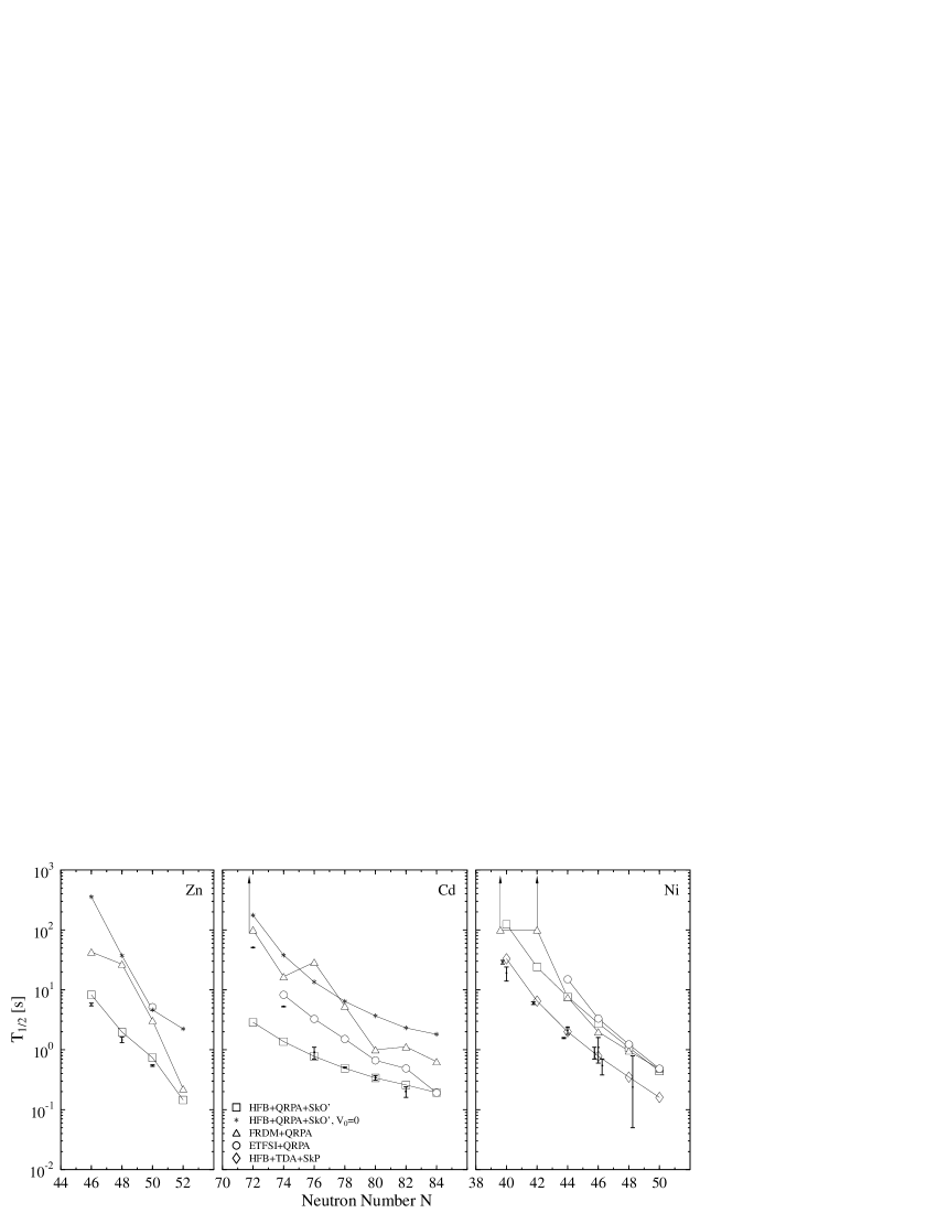
FIG. 6.: Comparison of calculated half-lives for Zn, Cd, and Ni isotopes with (HFB+QRPA+SKO’) and without (HFB+QRPA+SkO’, $V_{0}=0$) the residual particle-particle interaction, and results from Refs. [12] (FRDM+QRPA), [19] (ETFSI+QRPA), and [16] (HFB+TDA+SkP, only for the Ni isotopes), with experimental values taken from Ref. [54] where possible. For the nickel isotopes recent results from [51, 52] are shown as well. When predicted half-lives are larger than 100 s, the FDRM collaboration reports only this lower bound, which is marked here with arrows pointing up. The ETSFI collaboration reports half-lives only when the predicted deformation $\beta_{2}$ is less that 0.1.

where $\hat{\Pi}_{S=1,T=0}$ projects onto states with $S=1$ and $T=0$. We take the ranges $\mu_{1}$=1.2 fm and $\mu_{2}$=0.7 fm of the two Gaussians from the Gogny interaction [49], and choose the relative strengths $g_{1}$=1 and $g_{2}$=–2 so that the force is repulsive at small distances. The only remaining free parameter is $V_{0}$, the overall strength. Figure 3 depicts the rate of convergence of the predicted half-life of ¹²⁸Cd as a function of $V_{0}$ for the interaction (41) and for a $\delta$ interaction. The latter gives results that do not converge when we increase $e_{\rm cutoff}$, the upper limit on the (diagonal) energy of canonical states we include in the QRPA. The finite-range force behaves much better. The calculations reported below were carried out with the two-Gaussian force in Eq. (41) and with $e_{\rm cutoff}$=25  MeV for states above the Fermi surfaces (we include all states below the Fermi surfaces).

To fit the strength $V_{0}$, we use recently measured half-lives of neutron-rich nuclei in regions where the r-process path comes closest to the valley of stability (e.g., around ⁷⁸Ni) [50, 51, 52]). Fig. 4 displays the ratio of calculated-to-experimental lifetimes for three zinc isotopes and ⁸²Ge, all near $N$=50. The four lines intersect near a ratio of 1, showing that the experimental lifetimes can all be reproduced with a single value of the $T$=0 pairing strength, $V_{0}$=230 MeV. We use this interaction strength to predict the lifetimes of nuclei (in this region) that are still further from stability.

Fig. 5 shows the corresponding results for ^126,128,130Cd, all near $N$=82. The fit, while not as good here, is still reasonable and gives a best value for $V_{0}$ of about 170 MeV. At that value we slightly underestimate the lifetime of ¹²⁴Cd (by a factor of 0.6). For ¹²²Cd the discrepancy is greater — we underestimate its lifetime by a factor of 5 — but that nucleus has such a small $Q_{\beta^{-}}$–value that a small error in the strength distribution can have a large effect on the rate. We therefore adopt the value $V_{0}$=170 for the entire region. The reason the value of $V_{0}$ is so different here might be connected with the quality of the single-particle spectra and $Q$-values predicted by Skyrme forces, and with the simplicity of our $T$=0 pairing interaction. We may be compensating for such deficiencies by changing $V_{0}$. The fact that we have to change the $T$=0 pairing strength by such a large amount when going from $N$=50 to $N$=82 demonstrates the sensitivity of calculated beta decay rates to other parts of the effective interaction.

In the $N$=126 region there are not enough experimental data to support a fit of the $T$=0 pairing strength, so we use the same value ($V_{0}$=170 MeV) as in the $N$=82 region. This means that our predictions around $N$=126 are less reliable than in other regions (see, however, discussion in Sec. IV).

IV Results

FIG. 7.: Calculated half-lives of the neutron-rich Ni isotopes as a function of the strength of the $T$=0 pairing interaction.

A Measured half-lives

Figure 6 displays the results of our calculations for nuclei near the neutron closed shells, alongside the QRPA results without $T$=0 pairing ($V_{0}$=0), the results of Refs. [19, 16, 53], and measured half-lives [54]. (The predictions of Ref. [19] appear only when the nucleus is thought to have small deformation. Our numbers in these nuclei are more suspect than elsewhere, since we ignore deformation in our calculation.) Because we separately adjust the $T$=0 pairing strength in two regions, it is not surprising that our results are usually closer to experiment than those of global calculations in which parameter values are kept fixed. But the errors in the global calculations are systematic; they almost always overestimate the lifetimes. In the case of Ref. [12, 53], at least, we attribute the problem to the neglect of the $T$=0 pairing. As the figure shows, the results of Ref. [12, 53] are much closer to ours in most of the nuclei when we turn that force off.

In the Ni isotopes our lifetimes are also too large by factors of 3-5. Part of the reason is the weak sensitivity of these lifetimes to $V_{0}$, which in turn is due to the $Z$=28 and $N$=40 shell closures. The proton orbitals important for beta-decay are completely empty and therefore couple through $T$=0 pairing only to neutron orbitals that are at least partly empty. Because of the closed shell at $N$=40, the lowest such neutron orbit is $g_{9/2}$. But the $g_{9/2}$ neutrons can only decay into the proton $g$ orbitals, which are far above the proton Fermi surface. Thus no low-energy strength can be moved by the particle-particle interaction and the curves in Fig. 7, which shows the calculated half-lives of the nickel isotopes versus $V_{0}$, are all flat. They do not turn down until after the value of $V_{0}$ (230 MeV) that is suitable for the other nuclei in the region, and close to the point at which the QRPA collapses. Such behavior clearly means that SkO’ is not optimal in this region; the SkP interaction used in the calculations of Ref. [16] apparently better predicts single-particle properties and Q-values. Those calculations use no particle-particle force but, as discussed above, none is required in the Ni isotopes.

Our HFB + QRPA theory violates particle number conservation, with the result that pairing correlations artificially break down at closed shells. The predictions for nickel would probably be better in a number-conserving version of our approach (for the general formalism, see Ref. [55]).

FIG. 8.: The same as figure 7, but for $N=50$ isotones.

B Closed-neutron-shell r-process waiting points

The effects of $T$=0 pairing vary just as much in closed-neutron-shell nuclei along the r-process path as they do in the measured nuclei just discussed. In doubly magic nuclei like ⁷⁸Ni, ¹³²Sn, and ¹²²Zr, the $T$=0 pairing force is ineffective. On the other hand, when one takes away two protons from these nuclei, creating two holes in a high-spin orbit, the force has a large effect; the corresponding neutron orbit and its spin-orbit partner are not too far below the neutron Fermi surface and contain many neutrons, which both interact with the protons at their Fermi surface and decay to fill the two proton holes. The effect of adding two protons to a closed shell is a bit smaller. The several orbits above the closed proton shell have lower spin or are far from the Fermi surface, and their contributions tend to cancel. These points are illustrated in Fig. 8, which shows the dependence of the calculated half-lives of several $N=50$ isotones on $V_{0}$. The half-life of the doubly magic nucleus ⁷⁸Ni, of course, varies almost not at all, and we probably overpredict its lifetime slightly just as in the other Ni isotopes.

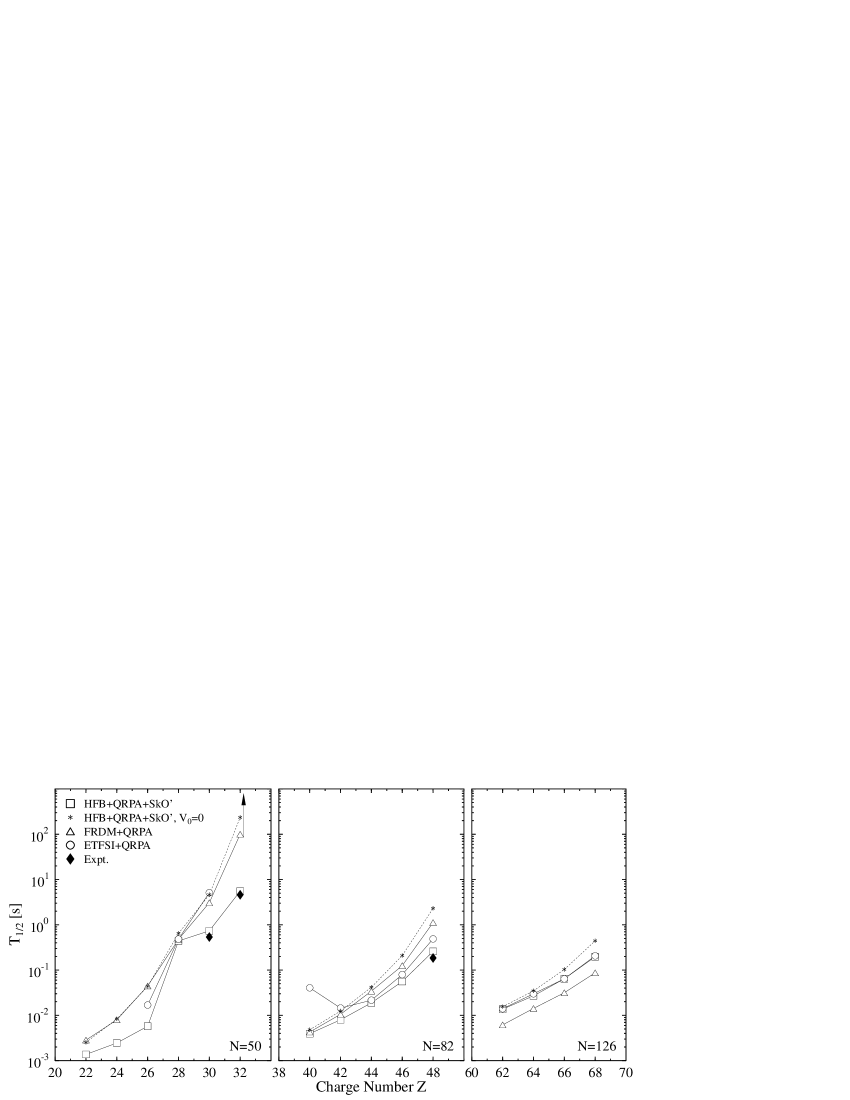
FIG. 9.: Predictions for the half-lives of closed neutron-shell nuclei along the r-process path. Our results appear with (HFB+QRPA+SKO’) and without (HFB+QRPA+SkO’, $V_{0}=0$)the $pn$ particle-particle interaction. Also plotted are the results of Ref. [12] (FRDM+QRPA), Ref. [19] (ETFSI+QRPA), and experimental data where available.

Figure 9 shows our predictions, together with those of other authors, for the half-lives of all the crucial even-even closed-neutron-shell nuclei along the r-process path. Our results agree fairly well with those of Ref. [12] for the very proton-poor nuclei (with $N=50$ and $N=82$) but less well for larger $Z$. The trend is due to the closed proton shells at $Z=20$, 28, 40, and 50, where the particle-particle force has little effect. Between these magic numbers, and particularly just below them (e.g., in ${}^{76}{\rm Fe}$), the differences can be large. To demonstrate again that they are due to $T$=0 pairing, we plot results once more with that component of the force switched off ($V_{0}$=0), a step that brings our results into agreement with those of Ref. [12] in nearly all nuclei with $N$=50 or 82.

As discussed in Sect. III C, there are no experimental data with which to fix $V_{0}$ near $N$=126. The lack of closed shells in this region suggests that half-lives will depend strongly on $V_{0}$. Our results with and without $T$=0 pairing, however, show that this is not the case. Even if we used much a smaller value of $V_{0}$, by extrapolating the drop in that parameter between $N$ = 50 and 82, the lifetimes would not change appreciably. In these heavy systems our results agree well with those of Ref. [19].

C Consequences for nucleosynthesis

The closed-neutron-shell nuclei are instrumental in setting abundances produced in the r-process; new predictions for their half-lives will have an effect on the results of r-process simulations. For $N$=$50$ and 82 our half-lives are usually shorter than the commonly employed half-lives of Ref. [12], and longer for $N$=$126$ Replacing those lifetimes with ours should therefore produce smaller $A\approx 80$ and 130 abundance peaks, and a larger $A\approx 195$ peak.

Without extending our calculations to other nuclei in the r-process network, however, we cannot draw quantitative conclusions from a simulation. Accordingly, we carry out only one simple r-process simulation here, comparing final abundance distributions obtained from the beta decay rates of Ref. [12] with those obtained from our calculations, leaving all other ingredients unchanged (We also change rates at $N$=84 and 86, by amounts equal to the change in corresponding nuclei with $N$=82.) By specifying an appropriate temperature and density dependence on time, we mock up conditions in the “neutrino-driven wind” from Type II supernovae, the current best guess for the r-process site.

The results appear in Fig. 10. As expected, the $A\approx 130$ peak shrinks noticeably. The $A\approx 195$ peak broadens with the new half-lives because abundances around $N$=126 are built up not just at the longest lived (most stable) nucleus produced, but at more neutron-rich $N$=126 nuclei as well. As a result, more nuclei are populated and the peak widens. By contrast, the $N$=50 peak (not shown in Fig. 10) does not change much; its shape depends largely on the half life of ⁷⁸Ni, which in our calculations is almost the same as in those of Ref. [12]. We have already pointed out, however, that both lifetimes are probably too long. It is therefore reasonable to expect larger changes at low $A$ than our simulation indicates.

Besides altering the distribution of abundances, smaller half-lives can shorten the time required for the r-process to synthesize all the elements. The process proceeds only as fast as material can move through “bottlenecks”, the especially long-lived isotopes at the three closed neutron shells. In many simulations the sum of the lifetimes of the bottleneck nuclei exceeds the expected duration of r-process conditions in neutrino-driven winds [56]. To see what our lifetimes do, we run a series of r-process simulations at different temperatures, with both the half lives of Ref. [12] and with those presented here. At low temperatures, for which neutron photodissociation rates are slower, the average nucleus is extremely neutron rich and so the change in beta half-lives does not have a large effect; the time required for the r-process drops by $\approx 15\%$. At higher temperatures, nuclei that are slightly less neutron-rich are produced, and our half-lives have a more significant impact, resulting in an r-process time about $50\%$ shorter. These high-temperature simulations have difficulty reproducing the observed abundance distribution, so we cannot at present take them very seriously. It might be possible, however, to alter other conditions so that the correct distribution is restored. In any case, quantitative insight will have to await more comprehensive calculations of beta decay.

FIG. 10.: Predicted abundances in a simulation of the r-process. The solid line corresponds to the rates of Ref. [12], and the dotted line to the rates obtained here around $N$=82 and 126. All other nuclear and astrophysical parameters are the same for the two lines. The crosses are observed solar-system abundances.

V Summary and conclusions

This work contains the first consistent application of the coordinate-space HFB+QRPA formalism to beta decay in heavy neutron-rich nuclei. Our approach fully accounts for the coupling between the nuclear mean field, pairing, and the particle continuum. In addition our results are based on one Hamiltonian; we use the same interaction, SkO’, in the HFB and the QRPA calculations.

Beta-decay half-lives depend on Q-values, shell structure, and the residual interaction. Much of the effect of the last ingredient is summarized by the Landau-Migdal parameter $g_{0}^{\prime}$. Apparently all Skyrme interactions commonly used in nuclear structure studies, including SkO’, have values of $g_{0}^{\prime}$ that fall well below the experimental estimate ($g_{0}^{\prime}$$\sim$1.8). As a result, the centroid of the GT strength distribution is usually too low. That this defect is not fatal is due to pairing. Like-nucleon pairing produces diffuse Fermi surfaces, which in turn allow $T$=0 pairing to pull strength down in energy. We can therefore compensate for a small $g_{0}^{\prime}$ by weakening the strength of the $T$=0 pairing interaction slightly . But we definitely cannot omit it altogether; as Fig. 6 shows, calculations that do almost always overestimate lifetimes.

As for the r-process itself, shorter beta-decay rates will have an impact, but just how much is not yet clear. Abundances certainly shift somewhat, and the time it takes to complete the r-process will shrink, perhaps substantially. But in order to explore these issues fully, one needs to know half-lives for all the waiting point nuclei, not just those at the closed shells. Other quantities that affect abundance distributions, particularly neutron separation energies, also have to be better understood [57, 58].

One virtue of our self-consistent framework is that many extensions and improvements can be made systematically. First, a new interaction, based on the concept of the energy density functional, can be developed. This force should be able to reproduce global nuclear observables, and at the same time yield a value of $g_{0}^{\prime}$ that is close to 1.8. Finding such a force will require abandoning some of the conventional relations between the ${\cal H}^{\rm even}_{\rm Sk}$ and ${\cal H}^{\rm odd}_{\rm Sk}$ components of the energy density [34]. Then the parameters of ${\cal H}^{\rm even}_{\rm Sk}$ can be adjusted to global nuclear properties while those of ${\cal H}^{\rm odd}_{\rm Sk}$ can be fit to spin-dependent properties ($g_{0}$, $g_{0}^{\prime}$, moments of inertia, etc.).

Following the development of a better interaction, one can both improve the calculations presented here and extend them to open-shell nuclei that are not spherical. The formalism might also to be developed so that particle-number and isospin conservation are at least partly restored. Finally, all the nuclear ingredients in r-process network simulations, including neutron-separation energies, should be based on the same effective Hamiltonian. Only then might our understanding of neutron rich nuclei be sufficient to predict details of the r-process abundance distribution. This paper is a first step towards that goal.

REFERENCES

- [1] E. M. Burbidge, G. R. Burbidge, W. A. Fowler, and F. Hoyle, Rev. Mod. Phys. 29, 547 (1957).
- [2] D. D. Clayton, Principles of stellar evolution and nucleosynthesis, (University of Chicago Press, Chicago, 1983).
- [3] J. K. Cowan, F.–K. Thielemann, and J. W. Truran, Phys. Rep. 208, 267 (1991).
- [4] B. S. Meyer, G. J. Mathews, W. M. Howard, S. E. Woosley, and R. D. Hoffman, Ap. J. 399, 656 (1992); S.E. Woosley, et al. Ap. J. 433 (1994) 229.
- [5] K.–L. Kratz, J.–P. Bitouzet, F.–K. Thielemann, P. Möller, and B. Pfeiffer, Ap. J. 403, 216 (1993).
- [6] J. Witti, H.–Th. Janka, and K. Takahashi, Astron. Astrophys. 286, 841 (1994); 286, 857 (1994).
- [7] P. B. Radha, D. J. Dean, S. E. Koonin, K. Langanke, and P.Vogel, Phys. Rev. C56, 3079 (1997).
- [8] G. Martinez–Pinedo, K. Langanke, and D. J. Dean, nucl-th/9811095.
- [9] J. Dobaczewski and W. Nazarewicz, Phil. Trans. R. Soc. Lond. A 356, 2007 (1998).
- [10] A.B. Migdal, Theory of Finite Fermi Systems and Applications to Atomic Nuclei (Interscience, New York, 1967).
- [11] S. Shlomo and G. Bertsch, Nucl. Phys. A243, 507 (1975).
- [12] P. Möller, and J. Randrup, Nucl. Phys. A514, 1 (1990).
- [13] H. Homma, E. Bender, M. Hirsch, K. Muto, H. V. Klapdor–Kleingrothaus, and T. Oda, Phys. Rev. C54, 2972 (1996).
- [14] M. Hirsch, A. Staudt, and H. V. Klapdor–Kleingrothaus, At. Data Nucl. Data Tables 44, 79 (1992).
- [15] M. Hirsch, A. Staudt, K. Muto, and H. V. Klapdor–Kleingrothaus, At. Data Nucl. Data Tables 53, 165 (1993).
- [16] J. Żylicz, J. Dobaczewski, Z. Szyma nski, Proceedings of 2nd International Conference on Exotic Nuclei and Atomic Masses, Bellaire, 1998 (to be published).
- [17] I. N. Borzov, S. A. Fayans, and E. L. Trykov, Nucl. Phys. A584, 335 (1995).
- [18] I. N. Borzov, S. A. Fayans, E. Krömer, D. Zawischa, Z. Phys. A 355, 117 (1996).
- [19] I. N. Borzov, S. Goriely, and J. M. Pearson, Nucl. Phys. A621, 307c (1997); http://astro.ulb.ac.be/iaa.htm.
- [20] I .N. Borzov, S. Goriely, and J. M. Pearson, Proc. of the Tours Symposium on Nuclear Physics III, Tours, France, September 2-5, 1997 M. Arnould, M. Lewitowicz, Yu. Ts. Oganessian, M. Ohta, H. Utsunomiya, and T. Wada [eds.], AIP Conference Proceedings 425, AIP, Woodbury and New York (1998), page 485.
- [21] Å Bohr, and B. R. Mottelson, Nuclear Structure Vol. II, Benjamin, New York, 1975.
- [22] A. S. Jensen, P. G. Hansen, and B. Jonson, Nucl. Phys. A431, 393 (1984).
- [23] P. Quentin and H. Flocard, Ann. Rev. Nucl. Part. Sci. 28, 523 (1978).
- [24] J. Dechargé, and D. Gogny, Phys. Rev. C 21, 1568 (1980).
- [25] P.–G. Reinhard, Rep. Prog. Phys. 52, 439 (1989).
- [26] P. Ring, Prog. Part. Nucl. Phys. 37, 193 (1996).
- [27] J. Dobaczewski, H. Flocard, and J. Treiner, Nucl. Phys. A422, 103 (1984).
- [28] J. Dobaczewski, W. Nazarewicz, T. R. Werner, J. F. Berger, C. R. Chinn, and J. Dechargé, Phys. Rev. C 53, 2809 (1996).
- [29] D. Vautherin and D.M. Brink, Phys. Rev. C 5, 626 (1972).
- [30] Y. M. Engel, D. M. Brink, K. Goeke, S. J. Krieger, and D. Vautherin, Nucl. Phys. A249, 215 (1975).
- [31] P. Bonche, H. Flocard, P.–H. Heenen, S. J. Krieger and M. S. Weiss, Nucl. Phys. A443 (1985) 39.
- [32] P.–G. Reinhard, Ann. Phys. (Leipzig) 1, 632 (1992).
- [33] J. Engel, P. Vogel, and M. Zirnbauer, Phys. Rev. C 37, 731 (1988).
- [34] J. Dobaczewski and J. Dudek, Phys. Rev. C 52, 1827 (1995); 55, 3177 (1997)E.
- [35] P.–G. Reinhard, and H. Flocard, Nucl. Phys. A584, 467 (1995).
- [36] T. Bürvenich, K. Rutz, M. Bender, P.–G. Reinhard, J. A. Maruhn, and W. Greiner, EPJ A3, 139 (1998).
- [37] J. W. Negele and D. Vautherin, Phys. Rev. C5, 1472 (1972).
- [38] J. W. Negele, in Effective Interactions and Operators in Nuclei, eds. J. Ehlers et al. (Springer-Verlag, Berlin, 1975), p. 270.
- [39] Nguyen Van Giai, and H. Sagawa, Phys. Lett. 106B (1981).
- [40] J. Bartel, P. Quentin, M. Brack, C. Guet, and H.–B. Håkansson, Nucl. Phys. A386, 79 (1982).
- [41] E. Chabanat, Ph. D. thesis, Lyon, 1995; E. Chabanat, P. Bonche, P. Haensel, J. Meyer, and R. Schaeffer, Nucl. Phys. A635, 231 (1998).
- [42] P.–G. Reinhard, D. J. Dean, W. Nazarewicz, J. Dobaczewski, J. A. Maruhn, and M. R. Strayer, in preparation.
- [43] F. Osterfeld, Rev. of. Mod. Phys. 64, 491 (1992).
- [44] P.–G. Reinhard, private communication.
- [45] See, e.g., J. Rapaport and E. Sugarbaker, Ann. Rev. Nucl. Part. Sci. 44, 109 (1994). and references therein.
- [46] G. Colò, Nguyen Van Giai, and H. Sagawa, Phys. Lett. B 363, 5 (1995).
- [47] J. Dobaczewski, W. Nazarewicz, and T. R. Werner, Phys. Scr. T56, 15 (1995).
- [48] K. Muto, E. Bender, and H.V. Klapdor, Z. Phys. A334, 47 (1989).
- [49] D. Gogny, in Proceedings of the International Conference on Nuclear Self-consistent Fields, Trieste, G. Ripka and M. Porneuf, eds., North Holland, Amsterdam, 1975.
- [50] Ch. Engelmann, F. Ameil, P. Armbruster, M. Bernas, S. Czajkowski, Ph. Dessagne, C. Dinzaud, H. Geissel, A. Heinz, Z. Janas, C. Kozhuharov, Ch. Miehé, G. Münzenberg, M. Pfützner, C. Röhl, W. Schwab, C. Stéphan, K. Sümmerer, L. Tassan–Got, B. Voss, Z. Phys. A 352, 251 (1995).
- [51] F. Ameil, M. Bernas, P. Armbruster, S. Czajkowski, Ph. Dessagne, H. Geissel, E. Hanelt, C. Kozhuharov, C. Miehé, C. Donzaud, A. Grewe, A. Heinz, Z. Janas, M. de Jong, W. Schwab, S. Steinhäuser, Eur. Phys. J. A1, 275 (1998).
- [52] S. Franchoo, M. Huyse, H. Kruglov, Y. Kudryavtsev, W. F. Mueller, R. Raabe, I. Reusen, P. van Duppen, J. Van Roosbroeck, L. Vermeeren, A. Wöhr, K.–L. Kratz, B. Pfeiffer, and W. B. Walters, Phys. Rev. Lett. 81, 3100 (1998).
- [53] P. Möller, J. R. Nix, and K.-L. Kratz, At. Data Nucl. Data Tables 66, 131 (1997).
- [54] R. B. Firestone, V. S. Shirley, S. Y. F. Chu, C. M. Baglin, and J. Zipkin, Table of Isotopes, John Wiley and Sons, New York, 1996.
- [55] C. Federschmidt and P. Ring, Nucl. Phys. A435, 110 (1985).
- [56] Y. Z. Qian, Nucl. Phys. A621, 363 (1997).
- [57] B. Chen, J. Dobaczewski, K.–L. Kratz, K. Langanke, B. Pfeiffer, F.–K. Thielemann, and P. Vogel, Phys. Lett. B355, 37 (1995).
- [58] B. Pfeiffer, K.–L. Kratz, and F.–K. Thielemann, Z. Phys. A357, 235 (1997).
- [59] T. Wakasa, H. Sakai, H. Okamura, H. Otsu, S. Fujita, S. Ishida, N. Sakamoto, T. Uesaka, Y. Satou, M. B. Greenfield, and K. Hatanaka, Phys. Rev. C 55, 2909 (1997).