Potential Energy Surfaces of Superheavy Nuclei

Abstract

We investigate the structure of the potential energy surfaces of the superheavy nuclei ${}^{258}_{158}{\rm Fm}_{100}$, ${}^{264}_{156}{\rm Hs}_{108}$, ${}^{278}_{166}{112}$, ${}^{298}_{184}{114}$, and ${}^{292}_{172}{120}$ within the framework of selfconsistent nuclear models, i.e. the Skyrme–Hartree–Fock approach and the relativistic mean–field model. We compare results obtained with one representative parametrisation of each model which is successful in describing superheavy nuclei. We find systematic changes as compared to the potential energy surfaces of heavy nuclei in the uranium region: there is no sufficiently stable fission isomer any more, the importance of triaxial configurations to lower the first barrier fades away, and asymmetric fission paths compete down to rather small deformation. Comparing the two models, it turns out that the relativistic mean–field model gives generally smaller fission barriers.

]

I Introduction

Superheavy nuclei are by definition those nuclei with charge numbers beyond the heaviest long–living nuclei that have a negligible liquid–drop fission barrier, i.e. they are only stabilized by shell effects [2, 3]. The stabilizing effect of the shell structure has been demonstrated in recent experiments at GSI [4, 5] and Dubna [6], where an island of increased stability in the vicinity of the predicted doubly magic deformed nucleus ${}^{270}_{162}{\rm Hs}$ [7, 8, 9] has been reached.

The full potential energy surface (PES) of superheavy nuclei is of interest as it allows to estimate the stability against spontaneous fission and to predict the optimal fusion path for the synthesis of these nuclei. Both features are of great importance for planning future experiments. There are numerous papers on the structure of the potential–energy surfaces of superheavy nuclei in macroscopic–microscopic models, see, e.g., [9, 10, 11], but only very few investigations in selfconsistent models so far. A systematic study of the deformation energy of superheavy nuclei along the valley of $\beta$ stability in the region $100\leq Z\leq 128$ and $150\leq N\leq 218$ in HFB calculations with the Gogny force $D1s$ under restriction to axially and reflection symmetric shapes was presented in [12]. The full potential energy surface in the $\beta$–$\gamma$ plane of a few selected nuclei as resulting from Skyrme–Hartree–Fock calculations in a triaxial representation is discussed in [13]. This investigation stresses the importance of non–axial shapes, that lower the fission barrier of some superheavy nuclei to half its value assuming axial symmetry. There is still no selfconsistent calculation of the deformation energy of superheavy nuclei allowing for reflection–asymmetric shapes.

In a series of papers we have demonstrated the uncertainties in the extrapolation of the shell structure to the region of superheavy nuclei within selfconsistent models [14, 15]. The reasons for the different behavior of parametrisations that work comparably well for conventional stable nuclei when extrapolated to large mass numbers can be traced to differences in the effective mass and the isospin–dependence of the spin–orbit interaction [16]. It is the aim of this paper to investigate the important degrees of freedom of the potential energy surface of superheavy nuclei for the example of a few selected nuclides, i.e. ${}^{258}_{158}{\rm Fm}_{100}$, ${}^{264}_{156}{\rm Hs}_{108}$, ${}^{278}_{166}{112}$, ${}^{298}_{184}{114}$, and ${}^{292}_{172}{120}$ within the framework of selfconsistent nuclear structure models, namely the relativistic mean–field model (RMF, for reviews see [17, 18]) and the nonrelativistic Skyrme–Hartree–Fock (SHF) approach (for an early review see [19]), in both cases including also reflection–asymmetric shapes.

II The framework

The comparison of the calculated binding energies of the heaviest known even–even nuclei with the experimental values [14, 15] has shown that the Skyrme parametrisation SkI4 and the relativistic force PL–40 are to be among the preferred parametrisations for the extrapolation to superheavy nuclei. The nonrelativistic force SkI4 is a variant of the Skyrme parametrisation where the spin–orbit force is complemented by an explicit isovector degree–of–freedom [20]. The energy functional and the parameters are presented in Appendix A 1. The modified spin–orbit force has a strong effect on the spectral distribution in heavy nuclei and produces a big improvement concerning the binding energy of superheavy nuclei [14, 15]. The RMF parametrisation PL–40 [21] aims at a best fit to nuclear ground–state properties with a stabilized form of the scalar nonlinear selfcoupling, see Appendix A 2 for details. It shares most properties with the widely used standard nonlinear force NL–Z [22].

Both models are implemented in a common framework sharing all the model–independent routines. The numerical procedure represents the coupled SHF and RMF equations on a grid in coordinate space using a Fourier definition of the derivatives and solves them with the damped gradient iteration method [23]. An axial representation allowing for reflection–asymmetric shapes is employed in most of the calculations, while a triaxial deformed representation is used to investigate the influence of non–axial configurations on the first barrier.

In both SHF and RMF the pairing correlations are treated in the BCS scheme using a delta pairing force [24] $V_{\rm pair}=V_{\rm p/n}\,\delta(\textbf{r}_{1}-\textbf{r}_{2})$, see Appendix A 3 for details. This pairing force has the technical advantage that the strengths $V_{\rm p/n}$ are universal numbers which hold throughout the chart of nuclei, different from the widely used seniority model, where the strengths need to be parametrised with $A$ dependence, and therefore in the description of a fission process would have to be interpolated between the values for the initial nucleus and averaged values for the fission fragments.

Furthermore, a center–of–mass correction is performed by subtracting a posteriori $E_{\rm c.m.}=\langle\hat{\textbf{P}}\rule{0.0pt}{6.8pt}^{2}_{\rm c.m.}\rangle/(2mA)$, see [18, 25], as done in the original fit of the parametrisations. This treatment of the center–of–mass correction is a fair approximation, its uncertainty for the heavy systems discussed here is smaller than $0.2\;{\rm MeV}$ [26]. The center–of–mass correction, however, has to be complemented by corrections for spurious rotational and vibrational modes as well. Their proper implementation is a very demanding task, as it requires the appropriate cranking masses. As done in most other mean–field calculations, we omit this detail. In the barrier heights, which we will discuss here, only the variation of these corrections with deformation enters. An estimate for these effects can be taken from a two–center shell model calculation of actinide nuclei [27, 28]: the amplitude of the corrections increases with increasing deformation, lowering the first barrier by approximately $0.5\;{\rm MeV}$ and the second barrier by $2\;{\rm MeV}$. There is an uncertainty due to the numerical solution of the equations of motion which is of the order of $0.1\;{\rm MeV}$ even for large deformations, thus negligible in our calculations. The prescription of pairing adds another uncertainty to the calculated binding energies. We use the same pairing scheme and force for all calculations with an optimized strength for each mean–field parametrisation. The use of a local pairing force improves the description of pairing correlations within the BCS scheme compared to a constant force or constant gap approach [29], and removes some problems concerning the coupling of continuum states to the nucleus. From possible variation of pairing recipes, we assume an uncertainty of the total binding energy of approximately $1\;{\rm MeV}$ [30].

In the following, we will present deformation energy curves calculated with a quadrupole constraint (for numerical details see [31]). In a constrained selfconsistent calculation all unconstrained multipole deformations (of protons and neutrons separately) are left free to adjust themselves to a minimum energy configuration within the chosen symmetry. Thus the selfconsistent description of the potential–energy surface takes many more degrees of freedom into account than the $3$-$5$ shape parameters that can be handled within macroscopic–microscopic calculations. The macroscopic–microscopic models have the additional technical disadvantage that, for the description of a fission process, several nucleon–number dependent terms in both the parametrisation of the macroscopic and the microscopic model have to be interpolated between the values for the compound system and the fragments (see, e.g., [9]), leading to an uncertainty of the binding energy in the intermediate region. It is to be noted, however, that there remains some open end concerning shapes also in the selfconsistent models as there might exist several local minima which are separated by a potential barrier. The numerical procedure solving the constrained mean–field equations converges usually to the next local minimum, depending on the initial state. And it requires experience as well as patient searches to make sure that one has explored all local minima in a given region.

The deformation energy curves presented in the following are shown versus the dimensionless multipole moments of the mass density which are defined as

$$\beta_{\ell}=\frac{4\pi}{3Ar_{0}^{\ell}}\;\langle r^{\ell}\,Y_{\ell 0}\rangle\quad\hbox{with $r_{0}=1.2\,A^{1/3}\;$fm.}$$

Note that these $\beta_{\ell}$ are computed as expectation values from the actual mass distribution of the nucleus and need to be distinguished from the generating deformation parameters which are used in the multipole expansion of the nuclear shape in macroscopic models [32]. Besides the description in terms of $\beta_{\ell}$, we will indicate the various shapes along the paths in all figures, by the mass density contours at $\rho_{0}=0.07\,{\rm fm}^{-3}$. Furthermore, when looking at potential energy surfaces, one should keep in mind that these are only the first indicators of the fission properties. A more detailed dynamical description requires also the knowledge of the collective masses along the path. This is, however, a very ambitious task which goes beyond the aim of this contribution. We intend here mainly a qualitative discussion of the potential landscape.

III Results and Discussion

Figure 1 shows results of a Skyrme–Hartree–Fock calculation with SkI4 for ${}^{258}{\rm Fm}$, a nucleus that is located at the lower end of the region of superheavy nuclei.

FIG. 1.: Valleys in the PES of ${}^{258}{\rm Fm}$ for SkI4 from calculations in axial symmetry with (“refl. sym.”) and without (“refl. asym.”) reflection symmetry. In the vicinity of the first barrier also the result from a non–axial calculation (“triaxial”) is shown. To give an impression of the nuclear shapes along the path, mass density contours at $\rho_{0}=0.07\;{\rm fm}^{-3}$ are drawn near the corresponding curves.

The strong shell effect in the prolate ground state lowers the binding energy of this nucleus by $19.3\;{\rm MeV}$ or $1\%$ compared to a spherical shape, demonstrating the importance of considering deformations for the calculation of the ground–state binding energies in this region of the chart of nuclei. The first barrier is lowered from 11.8 MeV to 7.7 MeV when allowing for triaxial configurations. But the preference for triaxial shapes at the top of the barrier disappears when going to both larger and smaller deformations. It is interesting to note that the axial solutions are not continuously connected from ground state through first minimum when using a constraint on the quadrupole moment, but develop in two branches distinguished by their hexadecapole moment. The ground–state branch has a diamond like shape with a $\beta_{4}$ much larger than the branch coming from outside. The continuous connection is established by the intermediate triaxial shapes.

FIG. 2.: Valleys in the PES of ${}^{264}{\rm Hs}$ for SkI4, drawn in the same manner as in Fig. 1.

FIG. 3.: Valleys in the PES of ${}^{264}{\rm Hs}$ for PL–40, drawn in the same manner as in Fig. 1.

The PES of ${}^{258}{\rm Fm}$ shows some significant deviations from the familiar double–humped fission barrier of the somewhat lighter nuclei in the plutonium region [33]. There is no superdeformed minimum in the PES that can be associated with a fission isomer because the second barrier vanishes in case of symmetric breakup. This is due to the strong shell effect of the closed spherical $Z=50$ shell in the two fragments, that reaches far inside to deformations as small as $\beta_{2}=1.0$, the usual location of the fission isomer. This is reflected in the evolution of shapes along the symmetric path, that look like two intersecting spheres. At large deformations around $\beta_{2}\approx 1.5$ a valley with finite mass asymmetry appears, which is separated from the symmetric valley by a small potential barrier, but $5\;\mbox{MeV}$ higher in energy. The occurrence of competing but well separated valleys and the consequences for fission or fusion complies with the results from macroscopic models, for a discussion see e.g. [9, 34].

Figure 2 shows the valleys in the PES of ${}^{264}{\rm Hs}$, at present the heaviest known even–even nucleus [35]. Although the fragments from a symmetric breakup of ${}^{264}{\rm Hs}$ are far from any shell closure, this channel of the PES keeps the characteristic structure of the PES of ${}^{258}{\rm Fm}$ like the absence of a fission isomer and the vanishing second barrier. The fission path will follow the reflection symmetric solution, that gives a much narrower barrier than the asymmetric solution. Although the first barrier has similar width and height as the first barrier of typical actinide nuclei, the absence of the second barrier will lower the lifetime against spontaneous fission dramatically. Like in the actinide region, the first barrier is a bit lowered if one allows for triaxial configurations. The reflection asymmetric solution does not lower the overall barrier, but it coexists far inside the barrier. This is a new feature occurring in the PES of many superheavy nuclei and was already found in macroscopic–microscopic calculations in the two–center shell model [36]. The asymmetric path connects the asymptotically separated combination ${}^{210}{\rm Po}+{}^{54}{\rm Cr}$ with the ground state, and corresponds to the fusion path. This combination of projectile and target differs only slightly from the experimentally successful choice ${}^{207}{\rm Pb}({}^{58}{\rm Fe},{\rm n}){}^{264}{\rm Hs}$ [35]. It reflects the strong shell effect of an asymmetric breakup with a heavy fragment in the region of doubly magic ${}^{208}{\rm Pb}$. It is interesting to compare that with the case of actinide nuclei: these have also a well developed asymmetric path which is, however, confined to large deformations and reaches only down to the outer barrier [31].

A calculation of the PES of ${}^{264}{\rm Hs}$ in the RMF using PL–40 gives qualitatively the same results, see Fig. 3, but there are some differences in details. The barrier is a bit smaller in height and width than for SkI4. The lowering of the barrier for PL–40 is due to the smaller shell effect for the ground–state configuration in this parametrisation. While for SkI4 this nucleus has a deformed proton magic number, PL–40 does not predict a shell closure for $Z=108$ at all, see [15]. The effect of non–axial configurations on the height of the barrier is of the same size as in SkI4.

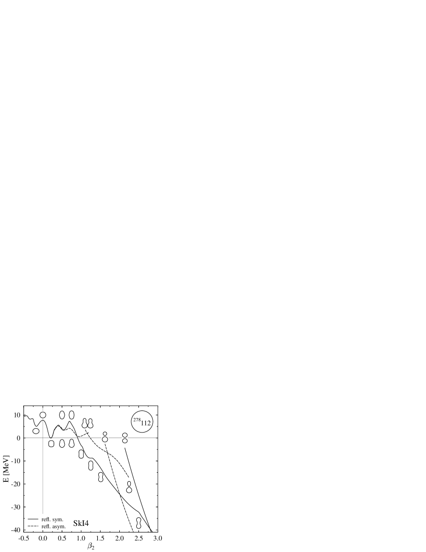
FIG. 4.: Valleys in the PES of ${}^{278}_{166}{\rm 112}$ for SkI4, drawn in the same manner as in Fig. 1.

As an example for a nucleus located at the upper border of the known chart of nuclei, Fig. 4 shows the valleys in the PES of ${}^{278}_{166}{\rm 112}$, calculated with SkI4. This nuclide corresponds to the compound nucleus in the cold fusion reaction ${}^{208}{\rm Pb}({}^{70}{\rm Zn},{\rm n}){}^{277}{112}$ which was used to synthesize the heaviest detected superheavy nucleus so far [5]. Although the proton number of this nucleus is close to the value $Z=114$ for the next spherical proton shell closure predicted by SkI4, its neutron number is quite far from the next predicted spherical neutron shell closure $N=184$ but close to the deformed shell closure $N=162$, that drives the nucleus to a strong prolate deformation with $\beta_{2}=0.22$, $\beta_{4}=-0.09$, see [15] for details. The PES of ${}^{278}_{166}{\rm 112}$ shares most overall features with the PES of ${}^{264}{\rm Hs}$, like the one–humped structure and the lowering of the first barrier due to asymmetric configurations, but there are some differences in detail. The (symmetric) fission barrier is narrower and slightly smaller (7.3 MeV compared with 10.6 MeV) than for ${}^{264}{\rm Hs}$. We have checked the effect of triaxial shapes and found that they are not effective to lower the first barrier for this superheavy nucleus. At superdeformed shapes $\beta_{2}\approx 0.5$ a spurious minimum develops in the symmetric barrier, that in reality is a saddle point, since the potential drops for asymmetric deformations. Note that the barrier is very soft in mass asymmetry in this region. Even at quadrupole deformations as small as $\beta_{2}=0.5$ the binding energy is nearly constant within the range $0<\beta_{3}<0.3$. The asymmetric path shows a rich substructure. There is a shallow minimum at $\beta_{2}\approx 0.9$, while around $\beta_{2}=1.2$, the results show a transition between two solutions with slightly different hexadecapole moment corresponding to shapes with differently pronounced “necks” but nearly constant mass asymmetry. The asymmetric valley corresponds to the breakup ${}^{210}{\rm Po}+{}^{68}{\rm Ni}$, that is quite close to the projectile–target combination used for the synthesis of this nuclide.

Axial and reflection symmetric calculations within the semi–microscopic “extended Thomas–Fermi–Strutinski integral method” (ETFSI) [37] that uses a Skyrme force, i.e. SkSC4, for the nuclear interaction as well, found superdeformed minima in the PES of this and many other superheavy nuclei in the region $Z\geq 112$ with $\beta_{2}\approx 0.45$ and a larger binding energy than the usual minima at small deformations. Our results indicate that these superdeformed minima vanish or will have a rather small fission barrier when reflection–asymmetric shapes are taken into account. Therefore the usual minimum in the PES at smaller $\beta_{2}$ has to be considered as the ground–state configuration, having a still sizeable first barrier and thus the larger fission half–life as compared to the competing minimum.

All nuclei discussed so far are located in the region of known superheavy nuclei. Now we want to look at possible candidates for the spherical doubly magic superheavy nucleus. As shown in [14, 15, 16], the predictions for doubly magic nuclei differ significantly between SHF and RMF. The RMF predicts ${}^{292}_{172}120$ to be doubly magic, while the extended Skyrme force SkI4 prefers ${}^{298}_{184}114$, the nucleus that has been predicted to be the center of the island of superheavy nuclei for a long time [2, 3]. Other Skyrme forces, however, do not predict any doubly magic spherical nuclei in this region at all or shift the center of the island of superheavy nuclei to ${}^{310}_{184}126$, for example the force SkP [14]. The PES of this nucleus, calculated with SkP allowing for triaxial shapes, is discussed in [13]. We now look at the two other candidates.

FIG. 5.: Valleys in the PES of ${}^{298}_{184}{114}$ for SkI4 and PL–40. Results from the calculations in different symmetries can be distinguished by the mass density contours which are drawn near the corresponding curves. In the vicinity of the first barrier for SkI4 also the result from a non–axial calculation is shown, that lowers the barrier.

Figure 5 shows the paths of minimum potential energy in the PES of ${}^{298}_{184}114$, calculated with SkI4 (solid line) and PL–40 (dotted line). While PL–40 shows only a weak neutron shell closure for this nucleus, ${}^{298}114$ is the spherical doubly magic superheavy nucleus predicted from SkI4. Therefore both forces lead to a spherical ground state of this nucleus, but with differently pronounced shell effects. In the figure, the PES from calculations with PL–40 is shifted with respect to SkI4 in such a way, that the (spurious) shallow symmetric minimum at $\beta_{2}\approx 0.6$ has the same energy in both models. For deformations larger than $\beta_{2}\approx 0.5$, both forces coincide in their prediction for the PES: The second barrier vanishes if asymmetric shapes are taken into account, but at large deformations the symmetric path is energetically favored. Even the shell fluctuations that lead to steps in the symmetric path are located at the same deformation for both forces. The significant difference between the potential energy surfaces occurs at small deformations $\beta_{2}<0.5$. The binding energy of the spherical configuration, measured from the reference point is lowered by $7\;{\rm MeV}$ for SkI4, but raised by approximately $1.3\;{\rm MeV}$ for PL–40. Nevertheless the spherical configuration is the ground–state for both forces. It remains to be noted that around $\beta_{2}\approx 0.3$ the barrier is slightly lowered for triaxial shapes, for SkI4 by approximately $3\;{\rm MeV}$, while for PL–40 the gain in energy is only a few hundred keV.

FIG. 6.: Valleys in the PES of ${}^{292}_{172}{120}$ for SkI4 and PL–40, drawn in the same manner as in Fig. 5.

As a final example, we consider the nucleus ${}^{292}_{172}{\rm 120}$ which has a spherical ground state and is a doubly magic system when computed with PL–40. Figure 6 shows its PES for PL–40 and SkI4. The PES confirms the spherical minimum for PL–40 whereas SkI4 prefers a slightly prolate ground state. It is to be remarked, however, that the actual ground state includes some quadrupole fluctuations around the minimum. In view of the weak deformation and small barrier at zero deformation it requires a more elaborate calculation including correlations to decide whether the true ground state will be spherical or deformed. A rather unexpected result is that the first barrier for PL–40 is indeed much lower than that for SkI4. This is a general result, that is also found for actinide nuclei like ${}^{240}{\rm Pu}$. The fission half–lives from PL–40 will thus be generally smaller and therefore ${}^{292}_{172}{\rm 120}$ will be more stable within SkI4 than with PL–40 although the latter predicts this as a doubly magic nucleus. Both forces predict a strongly competing second minimum which, however, cannot stabilize as a ground–state configuration (or serious isomer) because the low second barrier makes it extremely unstable against fission. This was already found in the previous examples and seems to be a general feature of superheavy nuclei. The shell effects cease to be strong enough to counterweight any more the strong decrease from Coulomb repulsion.

IV Conclusions

We have presented results of constrained selfconsistent calculations of superheavy nuclei within the Skyrme–Hartree–Fock and relativistic mean–field model. The global structure of the PES of superheavy nuclei shows some significant differences compared to the well–known double–humped fission barrier of heavy nuclei $90\leq Z<100$. The barrier of superheavy nuclei is only single–humped. For the lighter superheavy nuclei we still find that triaxial configurations lower the first barrier, i.e., the region between the ground state and $\beta_{2}\approx 1.0$. This effect vanishes for the heavier nuclei in the region $114\leq Z\leq 120$ discussed here, but reappears in the heavier nuclei around ${}^{310}_{184}126$ [13]. The second minimum (the fission isomer in the actinides) looses significance for all superheavy nuclei because it becomes unstable against (asymmetric) fission. Seen from the reverse side, it turns out that the shell structure of the final fragments influences the PES down to small deformations. The asymmetric channel with ²⁰⁸Pb as one fragment thus carries through deep into the first barrier. This corresponds most probably to the optimal fusion path whereas fission proceeds preferably along the symmetric shapes. The global patterns of the paths are less model dependent than for the actinides. Differences are most pronounced in the vicinity of the ground states. They are caused by differences in the detailed shell structure and lead to dramatically different predictions for shell closures and fission half lives. The existence and stability of superheavy nuclei is thus a most sensitive probe for the present mean–field models.

A Details of the Mean–Field Models

1 Skyrme Energy Functional

The Skyrme forces are constructed to be effective forces for nuclear mean–field calculations. In this paper, we use the Skyrme energy functional in the following form

$${\cal E}={\cal E}_{\rm kin}[\tau]+{\cal E}_{\rm Sk}[\rho,\tau,{\bf J}]+{\cal E}_{\rm C}[\rho_{p}]-{\cal E}_{\rm c.m.}$$

with

$${\cal E}_{\rm Sk} = \int\!{\rm d}^{3}r\bigg{(}\frac{b_{0}}{2}\rho^{2}-\frac{b^{\prime}_{0}}{2}\sum_{q}\rho_{q}^{2}+\frac{b_{3}}{3}\rho^{\alpha+2}-\frac{b^{\prime}_{3}}{3}\rho^{\alpha}\sum_{q}\rho_{q}^{2}$$

$$\quad+b_{1}\rho\tau-b^{\prime}_{1}\sum_{q}\rho_{q}\tau_{q}-\frac{b_{2}}{2}\rho\Delta\rho+\frac{b^{\prime}_{2}}{2}\sum_{q}\rho_{q}\Delta\rho_{q}$$

$$\quad-b_{4}\rho\nabla\cdot{\bf{J}}-b^{\prime}_{4}\sum_{q}\rho_{q}\nabla\cdot{\bf J}_{q}\bigg{)}$$

and $q\in\{{\rm p,n}\}$. $\rho_{q}$, $\tau_{q}$, and ${\bf J}_{q}$ denote the local density, kinetic density, and spin–orbit current, that are given by

$$\rho_{q} = \sum_{k\in\Omega_{q}}v_{k}^{2}|\psi_{k}|^{2},\quad\tau_{q}=\sum_{k\in\Omega_{q}}v_{k}^{2}|\nabla\psi_{k}|^{2},$$

$${\bf J}_{q} = -{\textstyle\frac{i}{2}}\sum_{k\in\Omega_{q}}v_{k}^{2}\Big{[}\psi_{k}^{\dagger}\,\nabla\times\hat{\sigma}\,\psi_{k}-(\nabla\times\hat{\sigma}\,\psi_{k})^{\dagger}\psi_{k}\Big{]}.$$

Densities without index denote total densities, e.g. $\rho=\rho_{\rm p}+\rho_{\rm n}$. The $\psi_{k}$ are the single–particle wavefunctions and $v_{k}^{2}$ the occupation probabilities calculated taking the residual pairing interaction into account, see Appendix A 3. ${\cal E}_{\rm kin}$ is the kinetic energy ${\cal E}_{\rm kin}=[\hbar^{2}/(2m)]\int\!{\rm d}^{3}r\,\tau$, while ${\cal E}_{\rm C}$ is the Coulomb energy including the exchange term in Slater approximation. The center–of–mass correction reads

$${\cal E}_{\rm c.m.}=\frac{1}{2mA}\bigl{\langle}\hat{\textbf{P}}\rule{0.0pt}{6.8pt}^{2}_{\rm c.m.}\bigr{\rangle},$$ (A1)

where $\hat{\textbf{P}}_{\rm c.m.}$ is the total momentum operator in the center–of–mass frame. The correction is calculated perturbatively by subtracting (A1) from the Skyrme functional after the convergence of the Hartree–Fock iteration. The parameters $b_{i}$ and $b^{\prime}_{i}$ used in the above definition are chosen to give a compact formulation of the energy functional, the corresponding mean–field Hamiltonian and residual interaction [38]. They are related to the more commonly used Skyrme force parameters $t_{i}$ and $x_{i}$ by

$$b_{0} = t_{0}\big{(}1+{\textstyle\frac{1}{2}}x_{0}\big{)},$$

$$b^{\prime}_{0} = t_{0}\big{(}{\textstyle\frac{1}{2}}+x_{0}\big{)},$$

$$b_{1} = {\textstyle\frac{1}{4}}\big{[}t_{1}\big{(}1+{\textstyle\frac{1}{2}}x_{1}\big{)}+t_{2}\big{(}1+{\textstyle\frac{1}{2}}x_{2}\big{)}\big{]},$$

$$b^{\prime}_{1} = {\textstyle\frac{1}{4}}\big{[}t_{1}\big{(}{\textstyle\frac{1}{2}}+x_{1}\big{)}-t_{2}\big{(}{\textstyle\frac{1}{2}}+x_{2}\big{)}\big{]},$$

$$b_{2} = {\textstyle\frac{1}{8}}\big{[}3t_{1}\big{(}1+{\textstyle\frac{1}{2}}x_{1}\big{)}-t_{2}\big{(}1+{\textstyle\frac{1}{2}}x_{2}\big{)}\big{]},$$

$$b^{\prime}_{2} = {\textstyle\frac{1}{8}}\big{[}3t_{1}\big{(}{\textstyle\frac{1}{2}}+x_{1}\big{)}+t_{2}\big{(}{\textstyle\frac{1}{2}}+x_{2}\big{)}\big{]},$$

$$b_{3} = {\textstyle\frac{1}{4}}t_{3}\big{(}1+{\textstyle\frac{1}{2}}x_{3}\big{)},$$

$$b^{\prime}_{3} = {\textstyle\frac{1}{4}}t_{3}\big{(}{\textstyle\frac{1}{2}}+x_{3}\big{)}.$$

The actual parameters for the parametrisation SkI4 used in this paper are

$$\begin{array}[]{rclrcl}t_{0}&=&-1855.827\,{\rm MeV}\,{\rm fm}^{3},&x_{0}&=&0.405082,\\ t_{1}&=&473.829\,{\rm MeV}\,{\rm fm}^{5},&x_{1}&=&-2.889148,\\ t_{2}&=&1006.855\,{\rm MeV}\,{\rm fm}^{5},&x_{2}&=&-1.325150,\\ t_{3}&=&9703.607\,{\rm MeV}\,{\rm fm}^{3+\alpha},&x_{3}&=&1.145203,\\ b_{4}&=&183.097\,{\rm MeV}\,{\rm fm}^{5},&b^{\prime}_{4}&=&-180.351\,{\rm MeV}\,{\rm fm}^{5}\end{array}$$

with ${\alpha=0.25}$. For the nucleon mass we use the value that gives $\hbar^{2}/(2m_{\rm p})=\hbar^{2}/(2m_{\rm n})=20.7525\,{\rm MeV}\,{\rm fm}^{2}$ for the constant entering ${\cal E}_{\rm kin}$.

2 Relativistic Mean–Field Model

For the sake of a covariant notation, it is better to provide the basic functional in the relativistic mean–field model as an effective Lagrangian density, which for this study is defined as

$${\cal L}_{\rm RMF}={\cal L}_{\rm N}+{\cal L}_{\rm M}+{\cal L}_{\rm NM}+{\cal L}_{\rm em},$$

where

$${\cal L}_{\rm M} = {\textstyle\frac{1}{2}}(\partial_{\mu}\Phi_{\sigma}\partial^{\mu}\Phi_{\sigma}-{\cal U}_{\rm nonl})$$

$$-{\textstyle\frac{1}{2}}\Big{[}{\textstyle\frac{1}{2}}(\partial_{\mu}\Phi^{\mbox{}}_{\omega,\nu}-\partial_{\nu}\Phi^{\mbox{}}_{\omega,\mu})\partial^{\mu}\Phi_{\omega}^{\nu}-m_{\omega}^{2}\Phi_{\omega,\mu}^{\mbox{}}\Phi_{\omega}^{\mu}\Big{]}$$

$$-{\textstyle\frac{1}{2}}\Big{[}{\textstyle\frac{1}{2}}(\partial_{\mu}{\mathbf{\Phi}}^{\mbox{}}_{\rho,\nu}-\partial_{\nu}{\mathbf{\Phi}}^{\mbox{}}_{\rho,\mu})\cdot\partial^{\mu}{\mathbf{\Phi}}_{\rho}^{\nu}-m_{\omega}^{2}{\mathbf{\Phi}}_{\rho,\mu}^{\mbox{}}\cdot{\mathbf{\Phi}}_{\rho}^{\mu}\Big{]},$$

$${\cal L}_{\rm NM} = -g_{\sigma}\Phi_{\sigma}\rho^{\rm s}-g_{\omega}\Phi_{\omega,\mu}\rho^{\mu}-g_{\rho}{\mathbf{\Phi}}_{\rho,\mu}\cdot{\mathbf{\rho}}^{\,\mu},$$

$${\cal U}_{\rm nonl} = {\textstyle\frac{1}{2}}\Delta m^{2}\biggl{(}\delta\Phi^{2}\log\biggl{[}\frac{\delta\Phi^{2}+(\Phi_{\sigma}-\Phi_{0})^{2}}{\delta\Phi^{2}+\Phi_{0}^{2}}\biggr{]}$$

$$\qquad\qquad\quad+\frac{2\Phi_{0}\;\delta\Phi^{2}\;\Phi_{\sigma}}{\delta\Phi^{2}+\Phi_{0}^{2}}\biggr{)}+{\textstyle\frac{1}{2}}m_{\infty}^{2}\Phi_{\sigma}^{2},$$

$${\cal L}_{\rm em} = -{\textstyle\frac{1}{2}}(\partial_{\mu}A_{\nu}-\partial_{\nu}A_{\mu})A^{\mu\nu}-eA_{\mu}\rho_{\rm p}^{\mu},$$

and ${\cal L}_{\rm N}$ is the free Dirac Lagrangian for the nucleons with nucleon mass $m_{\rm N}=938.9\,{\rm MeV}$, equally for protons and neutrons. The model includes couplings of the scalar–isoscalar ($\Phi_{\sigma}$), vector–isoscalar $(\Phi_{\omega,\mu}$), vector–isovector (${\mathbf{\Phi}}_{\rho,\mu}$), and electromagnetic ($A_{\mu}$) field to the corresponding scalar–isoscalar ($\rho^{\rm s}$), vector–isoscalar ($\rho^{\mu}$) and vector–isovector (${\mathbf{\rho}}^{\,\mu}$) densities of the nucleons. ${\cal U}_{\rm nonl}$ is the stabilized self–interaction of the scalar–isoscalar field, behaving like the standard ansatz for the nonlinearity at typical nuclear scalar densities, but with an overall positive–definite curvature to avoid instabilities at high scalar densities [18, 21]. The actual parameters of the parametrisation PL–40 are

$$\begin{array}[]{rclrcl}g_{\omega}&=&12.8861,&m_{\omega}&=&780.0\,{\rm MeV},\\ g_{\rho}&=&4.81014,&m_{\rho}&=&763.0\,{\rm MeV},\\ g_{\sigma}&=&10.0514,&\\ m_{\infty}^{2}&=&4.0\,{\rm fm}^{-2},&\Delta m^{2}&=&3.70015\,{\rm fm}^{-2},\\ \Phi_{0}&=&-0.111914\,{\rm fm}^{-1},&\delta\Phi&=&0.269688\,{\rm fm}^{-1}\end{array}$$

(we follow the usual convention $\hbar=c=1$ such that $197.3\,{\rm MeV}\equiv 1\,{\rm fm}^{-1}$). For the residual pairing interaction and the center–of–mass correction the same nonrelativistic approximations are used as in the SHF model.

3 Pairing Energy Functional

Pairing is treated in the BCS approximation using a delta pairing force [24], leading to the pairing energy functional

$${\cal E}_{\rm pair}=\frac{1}{4}\sum_{q\in\{{\rm p,n}\}}V_{q}\int\!{\rm d}^{3}r\;\chi_{q}^{2}\quad,$$ (A2)

where $\chi_{q}=-2\sum_{k\in\Omega_{q}>0}f_{k}u_{k}v_{k}\;|\psi_{k}|^{2}$ is the pairing density including state–dependent cutoff factors $f_{k}$ to restrict the pairing interaction to the vicinity of the Fermi surface [29]. $v_{k}^{2}$ is the occupation probability of the corresponding single–particle state and $u_{k}^{2}=1-v_{k}^{2}$. The strengths $V_{\rm p}$ for protons and $V_{\rm n}$ for neutrons depend on the actual mean–field parametrisation. They are optimized by fitting for each parametrisation separately the pairing gaps in isotopic and isotonic chains of semi–magic nuclei throughout the chart of nuclei. The actual values are

$$V_{\rm p}=-310\,{\rm MeV}\,{\rm fm}^{3},\quad V_{\rm n}=-323\,{\rm MeV}\,{\rm fm}^{3}$$

in case of SkI4 and

$$V_{\rm p}=-348\,{\rm MeV}\,{\rm fm}^{3},\quad V_{\rm n}=-346\,{\rm MeV}\,{\rm fm}^{3}$$

for PL–40. The pairing–active space $\Omega_{q}$ is chosen to include one additional oscillator shell of states above the Fermi energy with a smooth Fermi cutoff weight, for details see [29].

REFERENCES

- [1] Present address: Dept. of Physics and Astronomy, The University of North Carolina, CB 3255, Phillips Hall, Chapel Hill, NC 27599.
- [2] S. G. Nilsson, C. F. Tsang, A. Sobiczewski, Z. Szymanski, S. Wycech, C. Gustafson, I.–L. Lamm, P. Möller, B. Nilsson, Nucl. Phys. A131, 1 (1969).
- [3] U. Mosel, W. Greiner, Z. Phys. 222, 261 (1969).
- [4] S. Hofmann, V. Ninov, F. P. Hessberger, P. Armbruster, H. Folger, G. Münzenberg, H. J. Schött, A. G. Popeko, A. V. Yeremin, A. N. Andreyev, S. Saro, R. Janik, M. Leino, Z. Phys. A350, 277 (1995) and Z. Phys. A350, 281 (1995).
- [5] S. Hofmann, V. Ninov, F. P. Hessberger, P. Armbruster, H. Folger, G. Münzenberg, H. J. Schött, A. G. Popeko, A. V. Yeremin, S. Saro, R. Janik, M. Leino, Z. Phys. A354, 229 (1996).
- [6] Yu. A. Lazarev, Yu. V. Lobanov, Yu. Ts. Oganessian, V. K. Utyonkov, F. Sh. Abdullin, A. N. Polyakov, J. Rigol, I. V. Shirokovsky, Yu. S. Tsyganov, S. Iliev, V. G. Subbotin, A. M. Sukhov, G. V. Buklanov, B. N. Gikal, V. B. Kutner, A. N. Mezentsev, K. Subotic, J. F. Wild, R. W. Lougheed, K. J. Moody, Phys. Rev. C 54, 620 (1996).
- [7] Z. Patyk, A. Sobiczewski, Nucl. Phys. A533, 132 (1991).
- [8] P. Möller, J. R. Nix, Nucl. Phys. A549, 84, (1992).
- [9] P. Möller, J. R. Nix, J. Phys. G 20, 1681 (1994).
- [10] S. Ćwiok, A. Sobiczewski, Nucl. Phys. A342, 202 (1992)
- [11] R. Smolańczuk, J. Skalski, A. Sobiczewski, Phys. Rev. C 52, 1871 (1995).
- [12] J.–F. Berger, L. Bitaud, J. Dechargé, M. Girod, S. Peru–Dessenfants, Proceedings of the International Workshop XXXIV on Gross Properties of Nuclei and Nuclear Exitations, Hirschegg, Austria, January 1996. GSI, Darmstadt, 1996.
- [13] S. Ćwiok, J. Dobaczewski, P.–H. Heenen, P. Magierski, W. Nazarewicz, Nucl. Phys. A611, 211 (1996).
- [14] K. Rutz, M. Bender, T. Bürvenich, T. Schilling, P.–G. Reinhard, J. A. Maruhn, W. Greiner, Phys. Rev. C 56, 238 (1997).
- [15] T. Bürvenich, K. Rutz, M. Bender, P.–G. Reinhard, J. A. Maruhn, W. Greiner, accepted for publication in European Physical Journal A (1998).
- [16] M. Bender, K. Rutz, P.–G. Reinhard, J. A. Maruhn, W. Greiner, (in preparation).
- [17] B. D. Serot, J. D. Walecka, Adv. Nucl. Phys. 16, 1 (1986).
- [18] P.–G. Reinhard, Rep. Prog. Phys. 52, 439 (1989).
- [19] P. Quentin, H. Flocard, Ann. Rev. Nucl. Part. Sci. 28, 523 (1978).
- [20] P.–G. Reinhard, H. Flocard, Nucl. Phys. A584, 467 (1995).
- [21] P.–G. Reinhard, Z. Phys. A329, 257 (1988).
- [22] M. Rufa, P.–G. Reinhard, J. A. Maruhn, W. Greiner, M. R. Strayer, Phys. Rev. C 38, 390 (1989).
- [23] V. Blum, G. Lauritsch, J. A. Maruhn, P.–G. Reinhard, J. Comp. Phys. 100, 364 (1992).
- [24] S. J. Krieger, P. Bonche, H. Flocard, P. Quentin, M. S. Weiss, Nucl. Phys. A517, 275 (1990).
- [25] J. Friedrich, P.–G. Reinhard, Phys. Rev. C 33, 335 (1986).
- [26] K. W. Schmid, P.–G. Reinhard, Z. Phys. A 530, 283, (1991).
- [27] P.–G. Reinhard, Nucl. Phys. A306, 19 (1978).
- [28] P.–G. Reinhard, K. Goeke, Rep. Prog. Phys. 50, 1 (1987).
- [29] M. Bender, P.–G. Reinhard, K. Rutz, J. A. Maruhn, (in preparation).
- [30] P.–G. Reinhard, W. Nazarewicz, M. Bender, J. A. Maruhn, Phys. Rev. C 53, 2776 (1996).
- [31] K. Rutz, J. A. Maruhn, P.–G. Reinhard, W. Greiner, Nucl. Phys. A590, 680 (1995).
- [32] R. W. Hasse, W. D. Myers, Geometrical Relationships of Macroscopic Nuclear Physics, Springer, Berlin, 1988.
- [33] S. Bjørnholm, J. E. Lynn, Rev. Mod. Phys. 52, 725 (1980).
- [34] S. Ćwiok, P. Rozmej, A. Sobiczewski, Z. Patyk, Nucl. Phys. A491, 281 (1989).
- [35] G. Münzenberg, P Armbruster, G. Berthes, F. P. Heßberger, S. Hofmann, J. Keller, K. Poppensieker, B. Quint, W. Reisdorf, K.–H. Schmidt, H.–J. Schött, K. Sümmerer, I. Zychov, M. E. Leino, R. Hingmann, U. Gollerthan, E. Hanelt, Z. Phys. A328, 49 (1987).
- [36] A. Săndulescu, R. K. Gupta, W. Scheid, W. Greiner Phys. Lett. 60B, 225 (1976).
- [37] Y. Aboussir, J. M. Pearson, A. K. Dutta, F. Tondeur, At. Data Nucl. Data Tables 61, 127 (1995).
- [38] P.–G. Reinhard, Ann. Phys. (Leipzig) 1, 632 (1992).