Gauging of equations method.
I. Electromagnetic currents of three distinguishable particles

Abstract

We present a general method for incorporating an external electromagnetic field into descriptions of few-body systems whose strong interactions are described by integral equations. In particular, we address the case where the integral equations are those of quantum field theory and effectively sum up an infinite number of Feynman diagrams. The method involves the idea of gauging the integral equations themselves, and results in electromagnetic amplitudes where an external photon is effectively coupled to every part of every strong interaction diagram in the model. Current conservation is therefore implemented in the way prescribed by quantum field theory. We apply our gauging procedure to the four-dimensional integral equations describing a system of three distinguishable relativistic particles. In this way we obtain the expressions needed to calculate all possible electromagnetic processes of the three-body system. An interesting aspect of our results is the natural appearance of a subtraction term needed to avoid the overcounting of diagrams.

I Introduction

With the advent of new experimental facilities like the Thomas Jefferson National Accelerator Facility (TJAF), the Electron Stretcher Accelerator (ELSA), and the Mainz Microtron (MUMI), there is currently great interest in the use of photons and electrons to probe the structure of hadronic systems. In practice, this means using the electromagnetic probes to induce a variety of reactions amongst the hadrons. Here we shall be concerned with those reactions where effectively only one external photon is involved. This includes not only photoabsorption and photoproduction reactions, but also electron scattering and electroproduction when calculated to lowest order in the electromagnetic interaction. On the theoretical side such reactions are described by $\langle J^{\mu}\rangle$, the matrix element of the electromagnetic current operator, and it must ultimately be the goal of the theorist to construct models where $\langle J^{\mu}\rangle$ describes the experimental data as accurately as possible.

An essential constraint on $\langle J^{\mu}\rangle$ is that it must obey current conservation, expressed by the continuity equation $\partial_{\mu}\langle J^{\mu}\rangle=0$. Current conservation is a consequence of charge conservation and is therefore a fundamental property of any theory. On the other hand, because one uses models to approximate the full theory, current conservation is not guaranteed a priori. For this reason, much effort has been devoted to the question of how to impose current conservation within a particular model of strong interactions. In a seminal paper, Gross and Riska (GR) [1] have shown how to construct the conserved current of two nucleons described by the Bethe-Salpeter (BS) equation. By analysing specific meson-exchange diagrams of the BS kernel, they showed that current conservation is achieved when the two-nucleon interaction current is constructed by attaching photons to all possible places in the BS kernel. Although indispensable for the case of a two-body system, this result does not apply to systems consisting of three or more particles. There is also no straightforward way to use this result to construct the electromagnetic current of three particles even in the case where only two-body strong interactions are present.

Here we would therefore like to present a different method for constructing conserved currents that is applicable to any number of particles whose strong interaction processes are described by relativistic four-dimensional integral equations. This method involves a direct gauging of the equations themselves in the sense that a vector index $\mu$ is added to all terms of the equations in such a way that a linear equation in $\mu$-labelled quantities results. Proceeding in this way, we obtain integral equations for the gauged quantities of interest (e.g. the gauged Green function $G^{\mu}$ or the gauged scattering $t$-matrix $T^{\mu}$) expressed in terms of other gauged quantities that are known or that can be easily constructed (typically the gauged one-particle propagator $d^{\mu}$ and the gauged two-particle potential $v^{\mu}$). This approach, which we shall simply refer to as gauging the equations, results in the external photon being effectively coupled everywhere in the strong interaction model, so that current conservation is guaranteed.

Using this method for the case of two nucleons, we obtain that the hadronic current is a sum of matrix elements of the gauged nucleon propagators and the gauged BS kernel. Thus our result, in this case, coincides with the one of GR. However, our method is also easily applied to other systems. As the simplest strongly interacting system going beyond the two-body problem is that of three particles, we choose to illustrate the general nature of our gauging method by applying it to the relativistic three-body problem whose strong interactions are described by standard four-dimensional integral equations. That is, we consider systems like that of three nucleons or three quarks whose strong interaction processes do not involve coupling to the two-body sector. To keep the presentation as simple as possible we restrict the discussion to the case of three distinguishable particles. The gauging of three identical particles involves additional considerations of particle exchange symmetry and is the subject of the accompanying paper [2].

Although four-dimensional three-body equations have already been pursued numerically by Rupp and Tjon [3], there has not been a generalisation of the Gross-Riska result to the case of three particles. As a result, there is presently no rigorous derivation of the conserved current for a relativistic three-body systems. This paper is therefore devoted to showing how the gauging of relativistic three-body equations leads to gauge invariant expressions for the various electromagnetic transition currents of a three-particle system. It is a feature of our approach that the gauge invariance of our expressions is not imposed in an ad hoc fashion, but rather according to the way prescribed by field theory, namely by coupling photons to all possible places in the strong interaction model.

To show the flexibility of the gauging method, we apply it to two different relativistic three-body equations. The first of these is the integral equation for the $3\rightarrow 3$ Green function whose kernel is defined in terms of two-body potentials. This leads to three-body electromagnetic currents which are expressed in terms of two-body potentials $v$ and gauged two-body potentials $v^{\mu}$. In the second approach, we gauge the four-dimensional version of the Alt-Grassberger-Sandhas equations [4] in order to obtain electromagnetic currents that are expressed in terms of two-body $t$-matrices $t$ and gauged two-body $t$-matrices $t^{\mu}$. Our final results consist of gauge-invariant expressions for the electromagnetic current of the three-particle bound state, as well as the various electromagnetic transition currents of three particles. Thus, in the case of three distinguishable nucleons, our expressions describe the electromagnetic form factors of the bound $N\!N\!N$ system (³H), and the processes $Nd\rightarrow Nd\gamma$, $Nd\rightarrow\gamma N\!N\!N$, $\gamma^{3}$H$\rightarrow Nd$, and $\gamma^{3}$H$\rightarrow N\!N\!N$.

FIG. 1.: Examples of last cuts (dashed lines) in relativistic three- and four-body processes. (a) Ambiguous last cuts in the four-body problem. (b) Unique last cut in the three-body problem. (c) Ambiguous last cuts in electron scattering (top line) off three particles (bottom three straight lines). (d) The traditional picture of elastic electron scattering off a three-body bound state in impulse approximation. Interpreted as a Feynman graph (with the ellipses representing the bound state wave function), this diagram is consistent with the graph of (c) being included twice, once for each last cut shown. The diagram in (d) therefore contains overcounting.

A notorious problem plaguing many four-dimensional approaches is the overcounting of diagrams. For perturbation graphs, such overcounting can be corrected simply by subtracting the overcounted terms. However, when overcounting occurs within the scattering integral equations themselves, the way to solve the overcounting problem becomes highly non-trivial. Indeed, only recently has such an overcounting problem been solved in the context of four-dimensional integral equations for the $N\!N\!-\pi N\!N$ system [5, 6].

Overcounting can arise when reducible diagrams have ambiguous last cuts [5, 7, 8]. An example of an ambiguous last cut for the four-body problem is given in Fig. 1(a). Luckily, there is no overcounting in the four-dimensional scattering equations considered here. This is because of the purely three-body nature of our system (there is no coupling to two-body channels) which makes all last cuts unique - see Fig. 1(b). However, as soon as coupling to an external photon is made, the system effectively obtains coupling to the four-body sector and overcounting again becomes a possibility. To see this explicitly, consider the calculation of electron scattering off a three-body system in the relativistic impulse approximation. One contribution to this process is given in Fig. 1(c). The diagram shown contains ambiguous last cuts of the same type as in Fig. 1(a). This ambiguity needs to be carefully taken into account when summing the full perturbation series for the electron scattering process. For example, to find the expression describing electron scattering off a bound three-body system in the relativistic impulse approximation, one cannot simply use the direct generalisation of the non-relativistic expression as given diagrammatically in Fig. 1(d). Interpreted as a Feynman graph, this diagram overcounts interactions between the two spectator particles (the lowest two lines in the diagram) since such interactions are contained in both the initial and final three-body bound-state wave functions. This overcounting corresponds to the diagram of Fig. 1(c) being included twice, once for each last cut shown. Just this type of overcounting appears to be present in Rupp and Tjon’s calculation of the electromagnetic form factors of ${}^{3}\mbox{H}$.

An important feature of the gauging of equations method is that it not only attaches photons everywhere in the three-body amplitude, but it also does this without introducing any overcounting. Indeed, it is found that the gauging procedure itself gives rise to subtraction terms that effectively remove all overcounted contributions. In this way the complications brought about by ambiguous last cuts like that of Fig. 1(c) are taken care of automatically.

Preliminary results of the present paper (I) and the following paper (II) were first reported a few years ago [9]. In the meantime we have applied the gauging of equations method to the spectator formalism of Gross [10] to generate gauge invariant three-dimensional expressions describing any hadronic or quark system interacting with an external electromagnetic probe [11]. In particular, we have derived the three-dimensional expressions for the various electromagnetic transitions currents of the three-nucleon system within the spectator approach [12]. In this sense, the results of Ref. [12] can be considered as a gauge-invariant three-dimensional reduction of the four-dimensional results presented in I and II. We have also applied the gauging of equations method to the $N\!N\!-\pi N\!N$ system [13] where, as previously mentioned, the overcounting of diagrams provides an extra degree of complexity. For these works the present paper together with II form the basic theoretical foundation, and provide the references where all the missing details are given.

Although the power of the gauging of equations method is well demonstrated on the example of the three-body system considered here, it should be emphasized that the same method is just as easily applied to other strongly interacting systems (quark or hadron) including those where the number of particles is not conserved. Indeed this method has recently been used to gauge the $\pi N$ system [14], and as mentioned above, the $N\!N\!-\pi N\!N$ system [13].

As the gauging of equations method couples one external photon everywhere in the strong interaction model, it also forms the basis for exact descriptions of more complicated electromagnetic processes. For example, we have recently shown how to use this method to incorporate an internal photon into all possible places in a strongly interacting system [15]. The resulting expressions provide a way to calculate the complete set of lowest order electromagnetic corrections to any strong interaction model described by integral equations. Being complete, these electromagnetic corrections are therefore gauge invariant. The gauging method can also be used to describe processes with more than one photon. For example, by gauging a strong interaction scattering equation twice, we would obtain gauge invariant expressions for the corresponding Compton scattering process.

Finally, it is important to note that although we are concerned in this paper with the electromagnetic interaction for which gauge invariance (or current conservation) is a major issue, the gauging of equations method itself is totally independent of the type of external field involved. Thus all the expressions for transition currents developed in this paper hold also for cases where the external field is due to strongly or weakly interacting probes for which current is not conserved (of course the exact form of the gauged inputs would need to be chosen appropriately).

II GAUGING TWO DISTINGUISHABLE PARTICLES

A Gauging the two-particle Green function $G$

Gross and Riska [1] have shown how to construct a conserved current for the two-particle system described by the Bethe-Salpeter (BS) equation. In addition to the one-body current, which in general is not conserved, one also needs the two-body interaction current obtained by attaching a photon to each place inside all the Feynman diagrams defining the BS kernel. Such a current satisfies the two-body Ward-Takahashi (WT) identity [16] corresponding to the given model of strong interactions. On mass shell, this identity guarantees that the matrix element of the current operator satisfies the continuity equation. To obtain their result, Gross and Riska applied the one-body WT identities [17] to a number of meson exchange diagrams of the BS kernel. Here we would like to introduce a different method, that of gauging equations, by rederiving the Gross-Riska result for the case of two particles. In the subsequent sections, we shall illustrate the general nature of our method by applying it to the case of the three-particle system.

The two-body WT identity [16] can be written as

$$q_{\mu}G^{\mu}(k_{1}k_{2};p_{1}p_{2})=i[e_{1}G(k_{1}-q,k_{2};p_{1}p_{2})+e_{2}G(k_{1},k_{2}-q;p_{1}p_{2})$$ (2)

$$-G(k_{1}k_{2};p_{1}+q,p_{2})e_{1}-G(k_{1}k_{2};p_{1},p_{2}+q)e_{2}]$$

where $p_{1}p_{2}$ ($k_{1}k_{2}$) are initial (final) momenta of the particles, the photon is taken to be incoming with momentum $q$ so that $k_{1}+k_{2}=p_{1}+p_{2}+q$, $G$ is the full two-body Green function given by

$$(2\pi)^{4}\delta^{4}(p^{\prime}_{1}+p^{\prime}_{2}-p_{1}-p_{2})G(p^{\prime}_{1}p^{\prime}_{2};p_{1}p_{2})=\int d^{4}y_{1}d^{4}y_{2}d^{4}x_{1}d^{4}x_{2}$$ (4)

$$e^{i(p^{\prime}_{1}y_{1}+p^{\prime}_{2}y_{2}-p_{1}x_{1}-p_{2}x_{2})}\,\langle 0|T\Psi^{(1)}(y_{1})\Psi^{(2)}(y_{2})\bar{\Psi}^{(1)}(x_{1})\bar{\Psi}^{(2)}(x_{2})|0\rangle,$$

and $G^{\mu}$ is the corresponding five-point function

$$G^{\mu}(k_{1}k_{2};p_{1}p_{2})=\int d^{4}y_{1}d^{4}y_{2}d^{4}x_{1}d^{4}x_{2}$$ (6)

$$e^{i(k_{1}y_{1}+k_{2}y_{2}-p_{1}x_{1}-p_{2}x_{2})}\,\langle 0|T\Psi^{(1)}(y_{1})\Psi^{(2)}(y_{2})\bar{\Psi}^{(1)}(x_{1})\bar{\Psi}^{(2)}(x_{2})J^{\mu}(0)|0\rangle.$$

In the above, $\Psi^{(i)}$ and $\bar{\Psi}^{(i)}$ are Heisenberg fields of particle $i$, $T$ is the time ordering operator, $J^{\mu}$ is the quantised electromagnetic current operator, $|0\rangle$ the physical vacuum, and $e_{i}$ is the charge of the $i$-th particle. If the particles are isotopic doublets then $e_{i}$ includes an isospin factor, e.g. for nucleons $e_{i}=\frac{1}{2}[1+\tau_{3}^{(i)}]e_{p}$ where $\tau_{3}$ is the Pauli matrix for the third component of isospin, and $e_{p}$ is the charge of the proton.

For local field theory with distinguishable particles the electromagnetic current operator is given by

$$J^{\mu}(x)=-i\sum_{i=1}^{2}\frac{\partial{\cal L}}{\partial\left(\partial_{\mu}\Psi^{(i)}\right)}e_{i}\Psi^{(i)}+J^{\mu}_{\mbox{other}}(x)$$ (7)

where $J^{\mu}_{\mbox{other}}(x)$ consists of partial derivatives with respect to all other fields that are present in the Lagrangian ${\cal L}$. Note that we have used translational invariance to write Eq. (6) in terms of $J^{\mu}(0)$, and we have defined both $G$ and $G^{\mu}$ to be without total 4-momentum conserving $\delta$-functions. In Eq. (2) we have used a notation where the two-body Green function $G$ is labelled by four momentum variables even though only three are independent. Such notation allows us to write down the WT identity in an especially simple form that easily generalises to any numbers of particles.

FIG. 2.: Examples of the two types of Feynman diagram making up $G^{\mu}$. (a) A diagram that can be constructed by attaching a photon to a strong interaction diagram of $G$. (b) A diagram that cannot be constructed by attaching a photon to a diagram of $G$.

One can classify the contributions to $G^{\mu}$ into two groups [18]. The first of these consists of all Feynman diagrams that can be constructed from $G$ by attaching a photon to an appropriate diagram of $G$. An example is given in Fig. 2(a). The second group consists of diagrams that cannot be obtained from $G$ by attaching a photon, an example of which is given in Fig. 2(b). The special feature of the second group is that each contributing Feynman diagrams satisfies gauge invariance all on its own.

The goal of this paper is to show how to construct a gauge invariant $G^{\mu}$ by attaching a photon to all possible places in every Feynman diagram contributing to $G$. We shall refer to this attaching of photons everywhere as the gauging of $G$. On the other hand, diagrams like that of Fig. 2(b) are current conserving from the outset, and their construction is a separate problem which will not be considered here. Thus for the purposes of this paper, we take $G^{\mu}$ to be the result of the gauging of $G$, with the understanding that the neglected contributions can always be added separately without affecting the question of gauge invariance.

In a similar way, we use a superscript $\mu$ to indicate the vector quantity obtained by attaching photons everywhere to an amplitude or potential. However in this case we will require that no photons be attached to external lines of Feynman diagrams making up the amplitude; nevertheless, we shall still refer to the process of attaching the photons to all other places in the amplitude as gauging.

The WT identity is usually given in terms of the exact strong interaction Green functions of the underlying field theory. It follows that this identity must also be valid to any order with respect the strong interaction coupling constant. Here we would like to point out that the WT identity is also valid for any particular single diagram of the strong interaction. This is because one can always construct a Lagrangian with respect to which the diagram in question represents the only case of some given order of the strong interaction. In this case, the $G$ in the WT identity is given by just one diagram of the strong interaction, and $G^{\mu}$ is the sum of the diagrams obtained from $G$ by attaching the photon everywhere. In the same way, the WT identity is valid for any sum of diagrams included in $G$. Having this in mind, we consider $G$ to be given by the Bethe-Salpeter equation where the kernel $V$ is given by a model consisting of any number of connected two-particle irreducible Feynman diagrams.

We start by expressing $G$ in terms of its fully disconnected part $G_{0}$, and the kernel $V$:

$$G=G_{0}+G_{0}VG.$$ (8)

This is a symbolic equation that, for the case of two-particle scattering, represents a shorthand notation for

$$G(p^{\prime}_{1}p^{\prime}_{2};p_{1}p_{2})=G_{0}(p^{\prime}_{1}p^{\prime}_{2};p_{1}p_{2})+\int\frac{d^{4}r_{1}}{(2\pi)^{4}}\frac{d^{4}s_{1}}{(2\pi)^{4}}\,G_{0}(p^{\prime}_{1}p^{\prime}_{2};r_{1}r_{2})V(r_{1}r_{2};s_{1}s_{2})G(s_{1}s_{2};p_{1}p_{2})$$ (9)

where it is understood that $p^{\prime}_{1}+p^{\prime}_{2}=p_{1}+p_{2}=r_{1}+r_{2}=s_{1}+s_{2}$. In Eq. (9), neither the Green functions nor the kernel contain $\delta$-functions corresponding to total momentum conservation. Thus the disconnected Green function $G_{0}$ contains only one $\delta$-function and can be written as

$$G_{0}(p^{\prime}_{1}p^{\prime}_{2};p_{1}p_{2})=(2\pi)^{4}\delta^{4}(p^{\prime}_{1}-p_{1})d_{1}(p_{1})d_{2}(p_{2})=(2\pi)^{4}\delta^{4}(p^{\prime}_{2}-p_{2})d_{1}(p_{1})d_{2}(p_{2})$$ (10)

where $d_{i}$ is the dressed propagator of particle $i$. To save on notation we write Eq. (10) symbolically as

$$G_{0}=d_{1}d_{2}$$ (11)

where momentum labels and the momentum conserving $\delta$-function [together with factor $(2\pi)^{4}$] have been suppressed.

Eq. (8) is basically a topological statement regarding the two-particle irreducible structure of Feynman diagrams belonging to $G$; as such, it can be utilised directly to express the structure of the same Feynman diagrams, but with photons attached everywhere. Thus from Eq. (8) it immediately follows that

$$G^{\mu}=G_{0}^{\mu}+G_{0}^{\mu}VG+G_{0}V^{\mu}G+G_{0}VG^{\mu}.$$ (12)

This result expresses $G^{\mu}$ in terms of an integral equation, and illustrates what we mean by gauging an equation, in this case the gauging of Eq. (8). Implied in Eq. (12) is the result

$$[G_{0}VG]^{\mu}=G_{0}^{\mu}VG+G_{0}V^{\mu}G+G_{0}VG^{\mu},$$ (13)

which illustrates a rule for the gauging of products that is rather reminiscent of the product rule for derivatives. Although Eq. (13) follows from a topological argument, we shall postulate such a product rule to hold also in other cases where topological arguments may not be applicable. Again, Eq. (12) is a symbolic equation representing

$$G^{\mu}(k_{1}k_{2};p_{1}p_{2})=G^{\mu}_{0}(k_{1}k_{2};p_{1}p_{2})+\int\!\frac{d^{4}r_{1}}{(2\pi)^{4}}\frac{d^{4}s_{1}}{(2\pi)^{4}}\,G^{\mu}_{0}(k_{1}k_{2};r_{1}r_{2})V(r_{1}r_{2};s_{1}s_{2})G(s_{1}s_{2};p_{1}p_{2})$$ (16)

$$+\int\!\frac{d^{4}t_{1}}{(2\pi)^{4}}\frac{d^{4}u_{1}}{(2\pi)^{4}}\,G_{0}(k_{1}k_{2};t_{1}t_{2})V^{\mu}(t_{1}t_{2};u_{1}u_{2})G(u_{1}u_{2};p_{1}p_{2})$$

$$+\int\!\frac{d^{4}v_{1}}{(2\pi)^{4}}\frac{d^{4}w_{1}}{(2\pi)^{4}}\,G_{0}(k_{1}k_{2};v_{1}v_{2})V(v_{1}v_{2};w_{1}w_{2})G^{\mu}(w_{1}w_{2};p_{1}p_{2})\hskip 28.45274pt$$

where now the presence or absence of a photon with momentum $q$ needs to be taken into account in specifying the momentum conservation relations: $k_{1}+k_{2}=p_{1}+p_{2}+q$, where $k_{1}+k_{2}=t_{1}+t_{2}=v_{1}+v_{2}=w_{1}+w_{2}$, and $p_{1}+p_{2}=r_{1}+r_{2}=s_{1}+s_{2}=u_{1}+u_{2}$.

In Eq. (12), both $G^{\mu}$ and $G_{0}^{\mu}$ are obtained from the Green functions $G$ and $G_{0}$, respectively, by attaching photons everywhere. It is therefore important to note that the gauged potential $V^{\mu}$ is similarly obtained from $V$, but with no photons attached to external legs. This is because such contributions are already taken into account in the terms $G_{0}^{\mu}VG$ and $G_{0}VG^{\mu}$ of Eq. (12). Eqs. (8) and (12) are a set of linear integral equations for $G$ and $G^{\mu}$, and could be solved as such if $V$ and $V^{\mu}$ were given. However, we can also formally solve the equation for $G^{\mu}$, and thus express it directly in terms of $G$. Simple algebra gives:

$$G^{\mu}-G_{0}VG^{\mu}=G_{0}^{\mu}+G_{0}^{\mu}VG+G_{0}V^{\mu}G,$$

$$G^{\mu}=(I-G_{0}V)^{-1}\left[G_{0}^{\mu}(1+VG)+G_{0}V^{\mu}G\right]=G\left(G_{0}^{-1}G_{0}^{\mu}G_{0}^{-1}+V^{\mu}\right)G$$ (17)

where Eq. (8) was used in the last step. Defining the electromagnetic vertex function $\Gamma^{\mu}$ by

$$G^{\mu}=G\Gamma^{\mu}G,$$ (18)

Eq. (17) gives the essential result of this section:

$$\Gamma^{\mu}=\Gamma_{0}^{\mu}+V^{\mu}$$ (19)

where

$$\Gamma_{0}^{\mu}=G_{0}^{-1}G_{0}^{\mu}G_{0}^{-1}.$$ (20)

By gauging Eq. (11) one obtains

$$G_{0}^{\mu}=d_{1}^{\mu}d_{2}+d_{1}d_{2}^{\mu}$$ (21)

so that

$$\Gamma_{0}^{\mu}={\scriptstyle\Gamma}_{1}^{\mu}d_{2}^{-1}+d_{1}^{-1}{\scriptstyle\Gamma}_{2}^{\mu}$$ (22)

where ${\scriptstyle\Gamma}_{i}^{\mu}$ is the one-particle electromagnetic vertex function defined by the equation

$$d_{i}^{\mu}=d_{i}\,{\scriptstyle\Gamma}_{i}^{\mu}d_{i}.$$ (23)

Note that for nucleons, to lowest order in the strong interaction, ${\scriptstyle\Gamma}_{i}^{\mu}=e_{i}\gamma^{\mu}$ where $\gamma^{\mu}$ is a Dirac matrix. In Eq. (19) $\Gamma_{0}^{\mu}$ is thus the sum of single particle currents, and $V^{\mu}$ is the two-body interaction current of the given model. Eq. (19) is illustrated in Fig. 3. This is the essential result of Gross and Riska, and has been derived here using the gauging of equations method.

FIG. 3.: Illustration of Eq. (19) expressing the two-particle electromagnetic vertex function $\Gamma^{\mu}$ as a sum one-body currents and the two-particle interaction current.

B Ward-Takahashi identity for $G^{\mu}$

The validity of Eq. (12) for the gauging of $G$ is clear from the topological argument given above. We would nevertheless like to show explicitly that the $G^{\mu}$, constructed in this way, satisfies the WT identity. To do this, we first prove that the gauged potential $V^{\mu}$ satisfies the WT identity even though no photons are attached to its external legs. Using a shorthand notation defined by

$$G(k_{1}k_{2};p_{i}+q)=\left\{\begin{array}[]{ll}G(k_{1}k_{2};p_{1}+q,p_{2})&(i=1)\\ G(k_{1}k_{2};p_{1},p_{2}+q)&(i=2)\end{array}\right.$$ (24)

$$G(k_{i}-q;p_{1}p_{2})=\left\{\begin{array}[]{ll}G(k_{1}-q,k_{2};p_{1}p_{2})&(i=1)\\ G(k_{1},k_{2}-q;p_{1}p_{2})&(i=2)\end{array}\right.$$ (25)

we can write the WT identities for $G_{0}^{\mu}$ and the quantity $[G_{0}VG_{0}]^{\mu}$ as

$$q_{\mu}G_{0}^{\mu}(k_{1}k_{2};p_{1}p_{2})=i\sum_{i=1}^{2}[e_{i}G_{0}(k_{i}-q;p_{1}p_{2})-G_{0}(k_{1}k_{2};p_{i}+q)e_{i}],$$ (26)

$$q_{\mu}[G_{0}VG_{0}]^{\mu}(k_{1}k_{2};p_{1}p_{2})=i\sum_{i=1}^{2}[e_{i}G_{0}VG_{0}(k_{i}-q;p_{1}p_{2})-G_{0}VG_{0}(k_{1}k_{2};p_{i}+q)e_{i}].$$ (27)

Note that $[G_{0}VG_{0}]^{\mu}$ satisfies the WT identity because, unlike $V^{\mu}$, it has photons attached everywhere. Although Eq. (26) and Eq. (27) would be automatically true if field theory were being solved exactly, here we work within a strong interaction model specified by the input quantities $V$ and $G_{0}$; as such, these equations are assumed to be true by construction.

Using the product rule of Eq. (13), we have that

$$q_{\mu}[G_{0}VG_{0}]^{\mu}(k_{1}k_{2};p_{1}p_{2})=q_{\mu}G_{0}^{\mu}VG_{0}(k_{1}k_{2};p_{1}p_{2})+G_{0}\,q_{\mu}V^{\mu}G_{0}(k_{1}k_{2};p_{1}p_{2})$$ (29)

$$+G_{0}Vq_{\mu}G_{0}^{\mu}(k_{1}k_{2};p_{1}p_{2}).\hskip 14.22636pt$$

Writing out the integrals implied by this expression [see Eqs. (9) and (16)] and using Eqs. (26), (27) and (10), we obtain that

$$q_{\mu}V^{\mu}(k_{1}k_{2};p_{1}p_{2})=i\sum_{i=1}^{2}\left[e_{i}V(k_{i}-q;p_{1}p_{2})-V(k_{1}k_{2};p_{i}+q)e_{i}\right]$$ (30)

which is the WT identity for $V^{\mu}$. We may now use Eqs. (30) and (26) together with Eq. (19) to evaluate $q_{\mu}\Gamma^{\mu}(k_{1}k_{2};p_{1}p_{2})$. Taking into account that $G_{0}^{-1}-V=G^{-1}$, we obtain

$$q_{\mu}\Gamma^{\mu}(k_{1}k_{2};p_{1}p_{2})=i\sum_{i=1}^{2}\left[G^{-1}(k_{1}k_{2};p_{i}+q)e_{i}-e_{i}G^{-1}(k_{i}-q;p_{1}p_{2})\right].$$ (31)

Using this result and Eq. (18) it immediately follows that

$$q_{\mu}G^{\mu}(k_{1}k_{2};p_{1}p_{2})=i\sum_{i=1}^{2}\left[e_{i}G(k_{i}-q;p_{1}p_{2})-G(k_{1}k_{2};p_{i}+q)e_{i}\right],$$ (32)

thus proving the WT identity for the $G^{\mu}$ obtained by the gauging of equations method.

C Gauging the two-body bound-state wave function $\psi$

So far we have defined “gauging” to be the process where photons are attached to all places in perturbation diagrams. As Green functions and potentials have a diagrammatic interpretation, the gauging of these quantities has therefore a clear meaning. On the other hand, the bound-state wave function is a purely nonperturbative quantity, and thus cannot be associated with perturbation diagrams. One can nevertheless define the gauged bound-state wave function $\psi^{\mu}$ by formally gauging the bound-state Bethe-Salpeter equation using our product rule. Thus by gauging the equation

$$\psi=G_{0}V\psi$$ (33)

we obtain

$$\psi^{\mu}=\left(G_{0}V\right)^{\mu}\psi+G_{0}V\psi^{\mu}$$ (34)

in this way defining $\psi^{\mu}$. Here the symbol $\psi$ represents the two-body bound-state wave function $\psi_{P}(p_{1}p_{2})$ defined by

$$(2\pi)^{4}\delta^{4}(P-p_{1}-p_{2})\psi_{P}(p_{1}p_{2})=\int d^{4}x_{1}d^{4}x_{2}e^{i(p_{1}x_{1}+p_{2}x_{2})}\langle 0|T\Psi^{(1)}(x_{1})\Psi^{(2)}(x_{2})|P\rangle$$ (35)

where $P^{2}=m^{2}$ with $m$ being the mass of the bound two-body system. To save on notation, we do not write explicit spin and isospin labels in the state $|P\rangle$ nor in the wave function $\psi_{P}$; nevertheless, such labels (and if necessary, sums over such labels) are to be understood as implicitly present.

It is now straightforward to show that the $\psi^{\mu}$ defined by Eq. (34) is just the quantity $\psi^{\mu}(k_{1}k_{2};P)$ given by

$$\psi^{\mu}(k_{1}k_{2};P)=\int d^{4}x_{1}d^{4}x_{2}e^{i(k_{1}x_{1}+k_{2}x_{2})}\langle 0|T\Psi^{(1)}(x_{1})\Psi^{(2)}(x_{2})J^{\mu}(0)|P\rangle$$ (36)

where $k_{1}+k_{2}=P+q$. The proof of this proceeds as follows. Assuming the field theory under consideration admits a two-body bound state, the Green function $G$, defined by Eq. (4), exhibits a pole at $P^{2}=m^{2}$ where $P$ is the total four-momentum of the bound two-body system. Indeed from Eq. (4) it can be shown that as $P^{2}\rightarrow m^{2}$

$$G(p_{1}^{\prime}p_{2}^{\prime},p_{1}p_{2})\sim i\,\frac{\psi_{P}(p_{1}^{\prime}p_{2}^{\prime})\bar{\psi}_{P}(p_{1}p_{2})}{P^{2}-m^{2}}$$ (37)

where $P=p_{1}+p_{2}=p^{\prime}_{1}+p^{\prime}_{2}$ and $\psi_{P}$ is given by Eq. (35). Similarly from Eq. (6) one can show that for $P^{2}\rightarrow m^{2}$,

$$G^{\mu}(k_{1}k_{2},p_{1}p_{2})\sim i\,\frac{\psi^{\mu}(k_{1}k_{2};P)\bar{\psi}_{P}(p_{1}p_{2})}{P^{2}-m^{2}}.$$ (38)

with $\psi^{\mu}(k_{1}k_{2};P)$ given by Eq. (36). Using the last two results in Eq. (12), equating the residues at $P^{2}=m^{2}$, and writing $\psi^{\mu}$ as shorthand for $\psi^{\mu}(k_{1}k_{2};P)$, we obtain that

$$\psi^{\mu}\bar{\psi}=\left(G_{0}V\right)^{\mu}\psi\bar{\psi}+G_{0}V\psi^{\mu}\bar{\psi}.$$ (39)

We therefore deduce that the $\psi^{\mu}$ given by Eq. (36) does indeed satisfy Eq. (34). Eqs. (33) and (34) form a coupled set of equations which can be formally solved for $\psi^{\mu}$ giving

$$\psi^{\mu}\! = \!\left(1-G_{0}V\right)^{-1}\left(G_{0}V\right)^{\mu}\psi=GG^{-1}_{0}\left(G_{0}V\right)^{\mu}\psi$$ (40)

$$= \!G\left(G^{-1}_{0}G^{\mu}_{0}G^{-1}_{0}+V^{\mu}\right)\psi.$$ (41)

Recalling Eq. (19) we obtain

$$\psi^{\mu}=G\Gamma^{\mu}\psi.$$ (42)

Comparison with Eq. (18) shows that $\psi^{\mu}$ can be obtained from $G^{\mu}$ by taking the right-hand residue at the two-body bound-state pole [this of course is also obvious from Eq. (38)]. As such, $G_{0}^{-1}\psi^{\mu}$ is just the transition current describing the photo/electrodisintegration of the two-body bound state, as discussed shortly.

It is often convenient to work with the bound-state vertex function $\phi$ defined by the equations

$$\psi=G_{0}\phi\hskip 14.22636pt;\hskip 14.22636pt\bar{\psi}=\bar{\phi}G_{0}.$$ (43)

To gauge $\phi$ we follow the same idea as for the bound-state wave function, namely, we define $\phi^{\mu}$ by formally gauging the bound-state equation for $\phi$ [which follows from Eq. (33)]. In this way we obtain the coupled set of equations

$$\phi\! = \!VG_{0}\phi$$ (44)

$$\phi^{\mu}\! = \!\left(VG_{0}\right)^{\mu}\phi+VG_{0}\phi^{\mu}$$ (45)

which can be solved as above to give

$$\phi^{\mu}=G_{0}^{-1}G\left(VG_{0}\right)^{\mu}\phi.$$ (46)

Writing $(VG_{0})^{\mu}=V^{\mu}G_{0}+VG_{0}^{\mu}$ and $G_{0}^{-1}G=1+TG_{0}$ where $T$ is the $t$-matrix defined by

$$G=G_{0}+G_{0}TG_{0},$$ (47)

Eq. (46) reduces after some simple algebra to the result

$$\phi^{\mu}=(1+TG_{0})\Gamma^{\mu}\psi-\Gamma_{0}^{\mu}\psi.$$ (48)

D Ward-Takahashi identities for $\psi^{\mu}$ and $\phi^{\mu}$

The WT identity for $\psi^{\mu}$ follows from Eq. (42) and the WT identity for $\Gamma^{\mu}$, Eq. (31). Writing Eq. (42) in its full numerical form

$$\psi^{\mu}(k_{1}k_{2};P)=\int\frac{d^{4}t_{1}}{(2\pi)^{4}}\frac{d^{4}p_{1}}{(2\pi)^{4}}\,G(k_{1}k_{2};t_{1}t_{2})\Gamma^{\mu}(t_{1}t_{2};p_{1}p_{2})\psi(p_{1}p_{2};P),$$ (49)

we may use Eq. (31) to obtain

$$q_{\mu}\psi^{\mu}(k_{1}k_{2};P)=\int\frac{d^{4}t_{1}}{(2\pi)^{4}}\frac{d^{4}p_{1}}{(2\pi)^{4}}G(k_{1}k_{2};t_{1}t_{2})$$ (51)

$$\,i\sum_{i=1}^{2}\left[G^{-1}(t_{1}t_{2};p_{i}+q)e_{i}-e_{i}G^{-1}(t_{i}-q;p_{1}p_{2})\right]\psi(p_{1}p_{2};P).$$

Since $G^{-1}\psi_{P}=0$, the second term in the square brackets does not contribute and the above equation reduces down to the WT identity for $\psi^{\mu}$,

$$q_{\mu}\psi^{\mu}(k_{1}k_{2};P)=i\left[e_{1}\psi(k_{1}-q,k_{2};P)+e_{2}\psi(k_{1},k_{2}-q;P)\right].$$ (52)

The WT identity for $\phi^{\mu}$ is found in a similar manner. Written out numerically, Eq. (46) is

$$\phi^{\mu}(k_{1}k_{2};P)=\int\frac{d^{4}t_{1}}{(2\pi)^{4}}\frac{d^{4}p_{1}}{(2\pi)^{4}}\,[G_{0}^{-1}G](k_{1}k_{2};t_{1}t_{2})[VG_{0}]^{\mu}(t_{1}t_{2};p_{1}p_{2})\phi(p_{1}p_{2};P).$$ (53)

Note that the square brackets here indicate the resultant function to which the following momentum variables refer. As $[VG_{0}]^{\mu}$ is a gauged input, it satisfies the Ward-Takahashi identity from the outset. We can therefore write

$$q_{\mu}\phi^{\mu}(k_{1}k_{2};P)=\int\frac{d^{4}t_{1}}{(2\pi)^{4}}\frac{d^{4}p_{1}}{(2\pi)^{4}}\,[G_{0}^{-1}G](k_{1}k_{2};t_{1}t_{2})$$ (55)

$$i\sum_{i=1}^{2}\left\{e_{i}[VG_{0}](t_{i}-q;p_{1}p_{2})-[VG_{0}](t_{1}t_{2};p_{i}+q)e_{i}\right\}\phi(p_{1}p_{2};P).$$

The first term in the curly brackets can be integrated over $p_{1}$ using the fact that $VG_{0}\phi=\phi$. Similarly the second term in the curly brackets can be integrated over $t_{1}$ using the fact that $G_{0}^{-1}GVG_{0}=G_{0}^{-1}G-1$. Only one term survives,

$$q_{\mu}\phi^{\mu}(k_{1}k_{2};P)=\int\frac{d^{4}p_{1}}{(2\pi)^{4}}\,i\sum_{i=1}^{2}(2\pi)^{4}\delta^{4}(k_{i}-p_{i}-q)e_{i}\phi(p_{1}p_{2};P),$$ (56)

which gives the Ward-Takahashi identity for $\phi^{\mu}$:

$$q_{\mu}\phi^{\mu}(k_{1}k_{2};P)=i\left[e_{1}\phi(k_{1}-q,k_{2};P)+e_{2}\phi(k_{1},k_{2}-q;P)\right].$$ (57)

Note that neither of the WT identities of Eq. (52) nor Eq. (57) are zero, even for on mass shell $k_{1}$ and $k_{2}$. Thus neither $\psi^{\mu}$ nor $\phi^{\mu}$ obey current conservation.

E Two-body electromagnetic transition currents

To obtain the physical $t$-matrix for any reaction involving an electromagnetic probe interacting with a quark or hadronic system, it is sufficient to specify the corresponding matrix element of the electromagnetic current operator. We refer to such a matrix element simply as an electromagnetic transition current and denote it using the symbol $j^{\mu}$. Thus, for example, a process like two-nucleon Bremsstrahlung $N\!N\rightarrow\gamma N\!N$ is described by the $N\!N\rightarrow N\!N$ electromagnetic transition current $j_{00}^{\mu}$ given by

$$j_{00}^{\mu}=G_{0}^{-1}G^{\mu}G_{0}^{-1}.$$ (58)

The physical $t$-matrix is then found by contracting $j_{00}^{\mu}$ with the photon polarisation vector $\varepsilon_{\mu}$.

For processes with one two-body bound state, like deuteron photodisintegration, one determines the electromagnetic transition current $j_{0}^{\mu}$ from $G^{\mu}$ by taking the appropriate residue at the bound-state pole. Thus, to determine the $(ij)\rightarrow ij$ electromagnetic transition current describing the process $\gamma(ij)\rightarrow ij$ where a photon is absorbed on the bound state $(ij)$ producing free particles $i$ and $j$ in the final state, we take the residue of Eq. (18) on the right to obtain

$$j_{0}^{\mu} = G_{0}^{-1}G\Gamma^{\mu}\psi$$ (59)

$$= \!(1+TG_{0})\Gamma^{\mu}\psi$$ (60)

where $T$ is the off-shell two-body $t$-matrix. As noted previously, a comparison with Eq. (42) shows that the $(ij)\rightarrow ij$ electromagnetic transition current and the gauged bound-state wave function are simply related by

$$j_{0}^{\mu}=G_{0}^{-1}\psi^{\mu}.$$ (61)

It is also interesting to examine the relationship between $j_{0}^{\mu}$ and the gauged bound-state vertex function $\phi^{\mu}$. From Eq. (48) one immediately obtains that

$$j_{0}^{\mu}=\phi^{\mu}+\Gamma_{0}^{\mu}G_{0}\phi.$$ (62)

From this equation it is evident that the difference between $\phi^{\mu}$ and the electromagnetic transition current $j_{0}^{\mu}$ is that $\phi^{\mu}$ has no photons attached to external legs. This suggests that $\phi^{\mu}$ does not conserve current, while $j_{0}^{\mu}$ does. Indeed $q_{\mu}j_{0}^{\mu}=G_{0}^{-1}q_{\mu}\psi^{\mu}=0$ for on mass shell external legs since the momentum shifts ($-q$) contained in the WT identity for $\psi^{\mu}$, Eq. (52), ensure that the poles of $q_{\mu}\psi^{\mu}$ do not cancel the zero of $G_{0}^{-1}$.

Lastly we consider the case where an electromagnetic probe interacts with two particles which are bound in both initial and final states, for example elastic electron-deuteron scattering. Such processes are described by the electromagnetic bound-state current $j^{\mu}$ which can be found from Eq. (18) by taking residues at both the initial and final bound-state poles. As these bound states can have different total momenta, we write the bound-state current as

$$j^{\mu}=\bar{\psi}_{K}\Gamma^{\mu}\psi_{P}$$ (63)

where $K^{2}=P^{2}=m^{2}$. Current conservation for $j^{\mu}$ is obtained by using the WT identity for $\Gamma^{\mu}$, Eq. (31), and noting that $\bar{\psi}G^{-1}=G^{-1}\psi=0$.

III GAUGING THREE DISTINGUISHABLE PARTICLES

Having gauged the two-body system, we are ready to apply the gauging of equations method to the substantially more complicated case of three strongly interacting particles.

A Gauging the three-particle Green function

The Ward-Takahashi identity for three particles can be derived by following the same procedure as used by Bentz [16] for the two-particle case. One obtains

$$q_{\mu}G^{\mu}(k_{1}k_{2}k_{3};p_{1}p_{2}p_{3})=i[e_{1}G(k_{1}-q,k_{2}k_{3};p_{1}p_{2}p_{3})+e_{2}G(k_{1},k_{2}-q,k_{3};p_{1}p_{2}p_{3})$$ (66)

$$+e_{3}G(k_{1}k_{2},k_{3}-q;p_{1}p_{2}p_{3})-G(k_{1}k_{2}k_{3};p_{1}+q,p_{2}p_{3})e_{1}$$

$$-G(k_{1}k_{2}k_{3};p_{1},p_{2}+q,p_{3})e_{2}-G(k_{1}k_{2}k_{3};p_{1}p_{2},p_{3}+q)e_{3}].\hskip 28.45274pt$$

By extending the shorthand notation of Eqs. (24) and (25) to the case of three particles, the three-particle Ward-Takahashi identity can then be written more concisely as

$$q_{\mu}G^{\mu}(k_{1}k_{2}k_{3};p_{1}p_{2}p_{3})=i\sum_{i=1}^{3}[e_{i}G(k_{i}-q;p_{1}p_{2}p_{3})-G(k_{1}k_{2}k_{3};p_{i}+q)e_{i}].$$ (67)

Here $G$ is the full Green function of the three-particle system

$$(2\pi)^{4}\delta^{4}(p^{\prime}_{1}+p^{\prime}_{2}+p^{\prime}_{3}-p_{1}-p_{2}-p_{3})G(p^{\prime}_{1}p^{\prime}_{2}p^{\prime}_{3};p_{1}p_{2}p_{3})=\int d^{4}y_{1}d^{4}y_{2}d^{4}y_{3}d^{4}x_{1}d^{4}x_{2}d^{4}x_{3}$$ (69)

$$e^{i(p^{\prime}_{1}y_{1}+p^{\prime}_{2}y_{2}+p^{\prime}_{3}y_{3}-p_{1}x_{1}-p_{2}x_{2}-p_{3}x_{3})}\,\langle 0|T\Psi^{(1)}(y_{1})\Psi^{(2)}(y_{2})\Psi^{(3)}(y_{3})\bar{\Psi}^{(1)}(x_{1})\bar{\Psi}^{(2)}(x_{2})\bar{\Psi}^{(3)}(x_{3})|0\rangle$$

and $G^{\mu}$ is the corresponding seven-point function

$$G^{\mu}(k_{1}k_{2}k_{3};p_{1}p_{2}p_{3})=\int d^{4}y_{1}d^{4}y_{2}d^{4}y_{3}d^{4}x_{1}d^{4}x_{2}d^{4}x_{3}$$ (72)

$$e^{i(k_{1}y_{1}+k_{2}y_{2}+k_{3}y_{3}-p_{1}x_{1}-p_{2}x_{2}-p_{3}x_{3})}\langle 0|T\Psi^{(1)}(y_{1})\Psi^{(2)}(y_{2})\Psi^{(3)}(y_{3})\bar{\Psi}^{(1)}(x_{1})\bar{\Psi}^{(2)}(x_{2})\bar{\Psi}^{(3)}(x_{3})J^{\mu}(0)|0\rangle.$$

In practise, the Green function for three distinguishable particles is specified by the integral equation

$$G=G_{0}+G_{0}VG$$ (74)

where the potential $V$ is three-particle irreducible, and in the absence of three-body forces, is written as a sum of three disconnected potentials $V_{i}$:

$$V=V_{1}+V_{2}+V_{3}.$$ (75)

Here we use the usual spectator notation of three-body theory: defining $(ijk)$ to be a cyclic permutation of $(123)$, $V_{i}$ is the potential where particles $j$ and $k$ are interacting while particle $i$ is a spectator. Explicitly we have that

$$V_{i}(p^{\prime}_{1}p^{\prime}_{2}p^{\prime}_{3},p_{1}p_{2}p_{3})=v_{i}(p^{\prime}_{j}p^{\prime}_{k},p_{j}p_{k})d_{i}^{-1}(p_{i})(2\pi)^{4}\delta^{4}(p^{\prime}_{i}-p_{i})$$ (76)

where $v_{i}$ is the two-body potential between particles $j$ and $k$. Neither $V_{i}$ nor $v_{i}$ contain total momentum conserving $\delta$-functions, and the presence of $\delta^{4}(p^{\prime}_{i}-p_{i})$ in Eq. (76) is due purely to the disconnectedness of the potential $V_{i}$. In keeping with our shorthand notation, we write Eq. (76) as

$$V_{i}=v_{i}d_{i}^{-1}.$$ (77)

Our goal is to gauge Eq. (74) and in this way obtain the electromagnetic transition currents for the three-body system. As the gauging procedure is symbolically identical to that already presented for the two-body system, we conclude that Eqs. (18)-(20) apply also to the three-body system. Thus the seven-point function can be written as

$$G^{\mu}=G\Gamma^{\mu}G$$ (78)

where the electromagnetic vertex function for three particles is given by

$$\Gamma^{\mu}=G_{0}^{-1}G_{0}^{\mu}G_{0}^{-1}+V^{\mu}.$$ (79)

In the three-particle case, however, $V$ is given by Eqs. (75) and (77) so that

$$V^{\mu}=V_{1}^{\mu}+V_{2}^{\mu}+V_{3}^{\mu}.$$ (80)

To obtain $V_{i}^{\mu}$ all that is needed is to gauge the $V_{i}$ of Eq. (77). Yet because of the presence of the inverse propagator $d_{i}^{-1}$ in $V_{i}$, there is some question of how to do this consistently. An unambiguous answer is provided by gauging Eq. (74) with $V$ explicitly given by Eq. (75) and Eq. (77). In this case we write Eq. (74) as

$$G=G_{0}+\sum_{i}G_{0}V_{i}G=G_{0}+\sum_{i}D_{0i}v_{i}G$$ (81)

where $D_{0i}$ is the fully disconnected two-particle propagator defined by

$$D_{0i}=d_{j}d_{k}.$$ (82)

The gauging of Eq. (81) thus involves the term

$$(G_{0}V_{i}G)^{\mu}=(D_{0i}v_{i}G)^{\mu}=\left(D_{0i}^{\mu}v_{i}+D_{0i}v_{i}^{\mu}\right)G+D_{0i}v_{i}G^{\mu}.$$ (83)

Now using the fact that $D_{0i}^{\mu}=(G_{0}^{\mu}-D_{0i}d_{i}^{\mu})d_{i}^{-1}$, the above equation gives

$$(G_{0}V_{i}G)^{\mu} = \left[G_{0}^{\mu}V_{i}-G_{0}{\scriptstyle\Gamma}_{i}^{\mu}v_{i}+G_{0}\left(v_{i}^{\mu}d_{i}^{-1}\right)\right]G+G_{0}V_{i}G^{\mu}$$ (84)

$$= G_{0}^{\mu}V_{i}G+G_{0}\left(-{\scriptstyle\Gamma}_{i}^{\mu}v_{i}+v_{i}^{\mu}d_{i}^{-1}\right)G+G_{0}V_{i}G^{\mu}$$ (85)

from which it follows that

$$V_{i}^{\mu}=v_{i}^{\mu}d_{i}^{-1}-v_{i}{\scriptstyle\Gamma}_{i}^{\mu}.$$ (86)

It is seen that the same result would follow from gauging Eq. (77) directly using our product rule, as long as we use the prescription

$$\left(d_{i}^{-1}\right)^{\mu}=-{\scriptstyle\Gamma}_{i}^{\mu}.$$ (87)

This prescription can also be obtained by formally gauging the identity $d_{i}d_{i}^{-1}=1$ and taking $1^{\mu}=0$. The expression for the gauged potential $V_{i}^{\mu}$, Eq. (86), is illustrated in Fig. 4. The negative sign in front of the term $v_{i}{\scriptstyle\Gamma}_{i}^{\mu}$ may appear to be surprising, yet it is just what is needed to stop overcounting. Consider for example the gauging of the term $G_{0}VG$ appearing in Eq. (74): $(G_{0}VG)^{\mu}=G_{0}^{\mu}VG+G_{0}V^{\mu}G+G_{0}VG^{\mu}$. It is apparent that the rightmost diagram of Fig. 4 appears in each of the three terms $G_{0}^{\mu}VG$, $G_{0}V^{\mu}G$, and $G_{0}VG^{\mu}$. Thus the negative sign in question is needed to ensure that this diagram contributes only once to the gauging of $G_{0}VG$.

FIG. 4.: Illustration of Eq. (86) for the gauged disconnected potential $V_{i}^{\mu}$.

The fully disconnected three-particle Green function $G_{0}$ is given by

$$G_{0}=d_{i}d_{j}d_{k}$$ (88)

where two momentum conserving $\delta$-functions are implied in the used shorthand notation. Gauging this expressions gives

$$G_{0}^{\mu}=\sum_{i=1}^{3}d_{i}^{\mu}d_{j}d_{k}=\sum_{i=1}^{3}d_{i}^{\mu}D_{0i}$$ (89)

FIG. 5.: Illustration of Eq. (91) expressing the three-particle electromagnetic vertex function $\Gamma^{\mu}$ as a sum of one- and two-particle currents.

where the sum is over the three cyclic permutations of ($ijk$). The impulse term in Eq. (79) can then be written as

$$G_{0}^{-1}G_{0}^{\mu}G_{0}^{-1}=\sum_{i=1}^{3}{\scriptstyle\Gamma}_{i}^{\mu}D_{0i}^{-1}.$$ (90)

Using this and Eq. (86) in Eq. (79) then gives

$$\Gamma^{\mu}=\sum_{i=1}^{3}\left({\scriptstyle\Gamma}_{i}^{\mu}D_{0i}^{-1}+v_{i}^{\mu}d_{i}^{-1}-v_{i}{\scriptstyle\Gamma}_{i}^{\mu}\right)$$ (91)

which we illustrate in Fig. 5.

Noting that the full two-body Green function $D_{i}$ satisfies the equation

$$D_{i}=D_{0i}+D_{0i}v_{i}D_{i},$$ (92)

we can also write Eq. (91) as

$$\Gamma^{\mu}=\sum_{i=1}^{3}\left({\scriptstyle\Gamma}_{i}^{\mu}D_{i}^{-1}+v_{i}^{\mu}d_{i}^{-1}\right).$$ (93)

Eq. (93) [or equivalently Eq. (91)] is the main result of this section and extends the Gross-Riska result of Eq. (19) to the three-particle sector. It gives the precise way that the one- and two-body currents need to combine in order to obtain proper gauge invariance.

B Three-body bound-state current

The three-body bound-state current $j^{\mu}$ describes processes where a system of three strongly interacting particles is bound both before and after the interaction with an electromagnetic probe. Examples include elastic electron scattering from ³H and ³He [19], and elastic electron scattering from the proton considered as a bound three-quark system [20].

The bound-state current $j^{\mu}$ is found by taking left and right residues of Eq. (78) at the initial and final three-particle bound-state poles. With $M$ being the mass of the bound state, it can be shown that

$$G(p^{\prime}_{1}p^{\prime}_{2}p^{\prime}_{3};p_{1}p_{2}p_{3})\sim i\frac{\Psi_{P}(p^{\prime}_{1}p^{\prime}_{2}p^{\prime}_{3})\bar{\Psi}_{P}(p_{1}p_{2}p_{3})}{P^{2}-M^{2}}\hskip 28.45274pt\mbox{as}\hskip 14.22636ptP^{2}\rightarrow M^{2}$$ (94)

where $\Psi_{P}$ is the three-particle bound-state wave function defined by

$$(2\pi)^{4}\delta^{4}(P-p_{1}-p_{2}-p_{3})\Psi_{P}(p_{1}p_{2}p_{3})=$$ (96)

$$\int d^{4}x_{1}d^{4}x_{2}d^{4}x_{3}e^{i(p_{1}x_{1}+p_{2}x_{2}+p_{3}x_{3})}\langle 0|T\Psi^{(1)}(x_{1})\Psi^{(2)}(x_{2})\Psi^{(3)}(x_{3})|P\rangle.$$

Here $|P\rangle$ is the eigenstate of the full Hamiltonian corresponding to the three-particle bound state with momentum $P^{\mu}$. We thus find that

$$j^{\mu} = \bar{\Psi}_{K}\Gamma^{\mu}\Psi_{P}$$ (97)

$$= \sum_{i=1}^{3}\bar{\Psi}_{K}\left({\scriptstyle\Gamma}_{i}^{\mu}D_{0i}^{-1}+v_{i}^{\mu}d_{i}^{-1}-v_{i}{\scriptstyle\Gamma}_{i}^{\mu}\right)\Psi_{P}.$$ (98)

Note that the wave function $\Psi_{P}$ used here satisfies Eq. (94), and thus fulfils the normalisation condition (for distinguishable particles)

$$i\bar{\Psi}_{P}\frac{\partial}{\partial P^{2}}\left(G_{0}^{-1}-V\right)\Psi_{P}=1.$$ (99)

This result follows upon taking residues of the identity $G=GG^{-1}G$ and using the fact that $G^{-1}=G_{0}^{-1}-V$. By exposing the bound-state poles in the $G^{\mu}$ of Eq. (LABEL:G7pt), one finds that $j^{\mu}$ is also the matrix element of the current operator

$$j^{\mu}=\langle J^{\mu}\rangle\equiv\langle K|J^{\mu}(0)|P\rangle$$ (100)

where $K^{2}=P^{2}=M^{2}$. In terms of $j^{\mu}$, the familiar charge and magnetic form factors of spin-1/2 bound three-body systems are given by

$$F_{C}^{2}(q^{2}) = \sum|j^{0}|^{2}$$ (101)

$$F_{M}^{2}(q^{2}) = \frac{2M_{N}^{2}}{\mu^{2}Q^{2}}\sum\left[-\frac{Q^{2}}{4M^{2}}|j^{0}|^{2}+\left(1+\frac{Q^{2}}{4M^{2}}\right)|{\bf j}|^{2}\right]$$ (102)

where $\sum$ indicates a sum over final spins and an average over initial spins (recall that states $|P\rangle$ and wave functions $\Psi_{P}$ are to be understood as having implicit spin and isospin labels). In Eq. (102) $\mu$ is the magnetic moment of the bound state, $M_{N}$ is the nucleon mass, and $Q^{2}=-q^{2}$.

1 Role of subtraction term in the bound-state current

When used to calculate the bound-state current $j^{\mu}$, the role of the subtraction term in Eq. (91) is seen especially well by writing the bound-state wave function in terms of its usual Faddeev components:

$$\Psi=\sum_{i=1}^{3}\Psi_{i},$$ (103)

where $\Psi$ is written without a momentum subscript to save on notation, and where

$$\Psi_{i}=D_{0i}v_{i}\Psi.$$ (104)

For this purpose it is sufficient to consider just the one-body current contributions to $j^{\mu}$,

$$j^{\mu}_{\mbox{one-body}}=\sum_{i=1}^{3}\bar{\Psi}{\scriptstyle\Gamma}_{i}^{\mu}\left(D_{0i}^{-1}-v_{i}\right)\Psi.$$ (105)

Using Eq. (104) this then evaluates to

$$j^{\mu}_{\mbox{one-body}}=\sum_{i=1}^{3}\bar{\Psi}{\scriptstyle\Gamma}_{i}^{\mu}D_{0i}^{-1}(\Psi_{j}+\Psi_{k}).$$ (106)

This equation is not symmetrical with respect to the initial and final state wave functions. That this must be so can be seen as follows. The term ${\scriptstyle\Gamma}_{i}^{\mu}D_{0i}^{-1}$ corresponds to a first order electromagnetic interaction with particle $i$. During this interaction, particles $j$ and $k$ can be interacting, and this contribution is contained fully in the final state wave function $\bar{\Psi}$. To avoid overcounting, there must be no preceding $j-k$ interaction coming from the initial state wave function. This indeed is the case since, as is evident from Eq. (104), the very last interaction in $\Psi_{i}$ is between particles $j$ and $k$, and just this component is missing from the right-hand side (RHS) of Eq. (106).

Another way to write Eq. (106) is

$$j^{\mu}_{\mbox{one-body}}=\bar{\Psi}\Gamma^{\mu}_{0}\Psi-\sum_{i=1}^{3}\bar{\Psi}{\scriptstyle\Gamma}_{i}^{\mu}D_{0i}^{-1}\Psi_{i}$$ (107)

where $\Gamma^{\mu}_{0}=\sum_{i=1}^{3}{\scriptstyle\Gamma}_{i}^{\mu}D_{0i}^{-1}$ is the electromagnetic vertex function in the impulse approximation. In a three-dimensional approach, the term $\bar{\Psi}\Gamma^{\mu}_{0}\Psi$ would correspond to the correct expression for the total one-body current. In a four-dimensional approach, however, one needs to subtract the last term of Eq. (107) in order to avoid the overcounting just discussed. In this regard we note that the pioneering four-dimensional calculation of Ref. [3] used $\bar{\Psi}\Gamma^{\mu}_{0}\Psi$ as the expression for the one-body current, and therefore the results of this calculation contain overcounting.

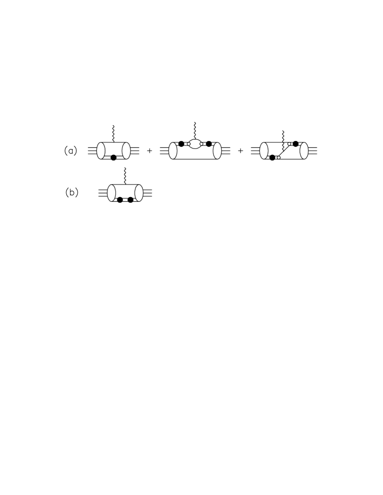
FIG. 6.: (a) The one-body electromagnetic current when two-body interactions are separable. (b) The overcounting term present in $\bar{\Psi}\Gamma_{0}^{\mu}\Psi$. The double-line with the black dot represents the dressed quasiparticle propagator $\tau$, the small open circle represents the separable potential form factor $h$, and the large ellipses represent the spectator bound-state form factor $X$.

Further insight into the nature of the overcounting problem can be gained by assuming, as was done in Ref. [3], that the input two-body potentials are separable. In this case we have

$$v_{i}=h_{i}\lambda h_{i}$$ (108)

where $h_{i}$ is the separable potential form factor with particle $i$ being a spectator. The two-body $t$-matrix is then given by

$$t_{i}=h_{i}\tau_{i}h_{i}$$ (109)

where

$$\tau_{i}^{-1}=\lambda^{-1}-h_{i}D_{0i}h_{i}.$$ (110)

For separable potentials we follow Ref. [3] and introduce the “spectator bound-state form factor” $X_{i}$ defined by

$$\Psi_{i}=G_{0}h_{i}\tau_{i}X_{i}.$$ (111)

As the Faddeev equation for the wave function components is

$$\Psi_{i}=D_{0i}t_{i}\left(\Psi_{j}+\Psi_{k}\right)$$ (112)

where $ijk$ are cyclic, it follows that

$$X_{i}=d_{i}^{-1}h_{i}\left(\Psi_{j}+\Psi_{k}\right).$$ (113)

Using these relations in Eq. (106) it is easy to show that

$$j^{\mu}_{\mbox{one-body}}=\sum_{i}\left(\bar{X}_{i}d_{i}^{\mu}\tau_{i}X_{i}+\sum_{j,k\neq i}\bar{X}_{j}\tau_{j}h_{j}D_{0i}d_{i}^{\mu}h_{k}\tau_{k}X_{k}\right)$$ (114)

which has a straightforward graphical interpretation. Depicted in Fig. 6(a) are the topologically distinct contributions to the sums in Eq. (114). One can similarly write

$$\bar{\Psi}\Gamma_{0}^{\mu}\Psi=\sum_{i}\left(\bar{X}_{i}d_{i}^{\mu}\tau_{i}X_{i}+\sum_{j,k\neq i}\bar{X}_{j}\tau_{j}h_{j}D_{0i}d_{i}^{\mu}h_{k}\tau_{k}X_{k}+\bar{X}_{i}d_{i}^{\mu}\tau_{i}\lambda_{i}^{-1}\tau_{i}X_{i}\right)$$ (115)

which compared to the previous equation, contains an extra term given by

$$\bar{\Psi}{\scriptstyle\Gamma}_{i}^{\mu}v_{i}\Psi=\sum_{i}\bar{X}_{i}d_{i}^{\mu}\tau_{i}\lambda_{i}^{-1}\tau_{i}X_{i}.$$ (116)

This term, depicted in Fig. 6(b), represents what is being overcounted in Eq. (115). Considering this overcounting term together with the first term in Eq. (115) [depicted by the first term in Fig. 6(a)], we see that the role of the overcounting term is to overdress the quasiparticle propagator while the spectator particle is being gauged. Thus, in the separable case, the use of the expression $\bar{\Psi}\Gamma_{0}^{\mu}\Psi$ to calculated the one-body electromagnetic current is equivalent to overdressing the quasiparticle propagator in the first term of Fig. 6(a).

2 Gauge invariance of the bound-state current

To prove the gauge invariance of Eq. (98) for the three-body bound-state current, it is convenient to use a symbolic notation for the WT identities. To do this we introduce the operators $\hat{e}_{i}$ whose numerical form is defined by

$$\hat{e}_{i}(k_{1}k_{2}k_{3},p_{1}p_{2}p_{3})=ie_{i}(2\pi)^{12}\delta^{4}(k_{i}-p_{i}-q)\delta^{4}(k_{j}-p_{j})\delta^{4}(k_{k}-p_{k})$$ (117)

where $ijk$ represents a cyclic ordering of $123$. Then the WT identities for the gauged two-body potential and gauged one-particle propagator can be written in three-particle space in terms of commutators as

$$q_{\mu}v^{\mu}_{i}I_{i}=[\hat{e}_{j}+\hat{e}_{k},v_{i}],\hskip 28.45274ptq_{\mu}d^{\mu}_{i}I_{j}I_{k}=[\hat{e}_{i},d_{i}]$$ (118)

where $I_{i}$, $I_{j}$, and $I_{k}$ are unit operators in the space of particles $i$, $j$, and $k$, respectively.

Writing Eq. (91) in the form

$$\Gamma^{\mu}=\sum_{i=1}^{3}\left(d^{-1}_{i}d^{\mu}_{i}d^{-1}_{i}d^{-1}_{j}d^{-1}_{k}+v_{i}^{\mu}d^{-1}_{i}-v_{i}d^{-1}_{i}d^{\mu}_{i}d^{-1}_{i}\right)$$ (119)

and using the WT identities of Eq. (118), the first term on the RHS of Eq. (119) gives

$$q_{\mu}\sum_{i=1}^{3}d^{-1}_{i}d^{\mu}_{i}d^{-1}_{i}d^{-1}_{j}d^{-1}_{k}=-[\hat{e},G_{0}^{-1}]$$ (120)

where

$$\hat{e}=\hat{e}_{1}+\hat{e}_{2}+\hat{e}_{3}.$$ (121)

Similarly for the last two terms of Eq. (119) we have that

$$q_{\mu}\left(v^{\mu}_{i}d^{-1}_{i}-v_{i}d^{-1}_{i}d^{\mu}_{i}d^{-1}_{i}\right)=[\hat{e}_{j}+\hat{e}_{k},v_{i}]d^{-1}_{i}+v_{i}[\hat{e}_{i},d_{i}^{-1}]=[\hat{e},v_{i}d^{-1}_{i}]$$ (122)

and therefore

$$q_{\mu}\sum_{i=1}^{3}\left(v^{\mu}_{i}d^{-1}_{i}-v_{i}d^{-1}_{i}d^{\mu}_{i}d^{-1}_{i}\right)=[e,V]$$ (123)

where $V$ is the full potential as given by Eq. (75). We have thus shown that

$$q_{\mu}\Gamma^{\mu}=-[\hat{e},G^{-1}]$$ (124)

where $G^{-1}=G_{0}^{-1}-V$ is the inverse of the full Green function. It is recognised that Eq. (124) is just the shorthand three-particle version of the two-particle result given in Eq. (31). Current conservation and therefore the gauge invariance of the bound-state current follows immediately. It is worth noting that the presence of the subtraction term [last term in Eq. (119)] is essential for current conservation.

3 Generalization to all transition currents

Electromagnetic currents for all possible transitions can be constructed by following the same procedure as above for the three-body bound-state current. That is, one can begin with the expression $G^{\mu}=G\Gamma^{\mu}G$ and then take residues at the relevant initial and final state poles. In this respect it is important to note that the Green function $G$ has poles corresponding not only to single particle propagators and three-body bound states, but also to two-body bound states. For example, it can be shown that in the vicinity of a two-body bound state of particles 2 and 3

$$G(k_{1}k_{2}k_{3},p_{1}p_{2}p_{3})\sim i\frac{\psi_{K_{1}}(k_{2}k_{3})d(k_{1})}{K_{1}^{2}-m^{2}}\bar{\Psi}^{\mbox{out}}_{K_{1}k_{1}}(p_{1}p_{2}p_{3})\hskip 28.45274pt\mbox{as}\hskip 28.45274ptK_{1}^{2}\rightarrow m^{2}$$ (125)

where $m$ is the bound-state mass of particles 2 and 3, and $K_{1}=k_{2}+k_{3}$. Similarly

$$G(k_{1}k_{2}k_{3},p_{1}p_{2}p_{3})\sim i\Psi^{\mbox{in}}_{P_{1}p_{1}}(k_{1}k_{2}k_{3})\frac{d(p_{1})\bar{\psi}_{P_{1}}(p_{2}p_{3})}{P_{1}^{2}-m^{2}}\hskip 28.45274pt\mbox{as}\hskip 28.45274ptP_{1}^{2}\rightarrow m^{2}$$ (126)

where $P_{1}=p_{2}+p_{3}$. The seven-point function $G^{\mu}$ has the same poles as $G$ and one can show, for example, that in the vicinity of these poles

$$G^{\mu}(k_{1}k_{2}k_{3},p_{1}p_{2}p_{3})\sim i\frac{\psi_{K_{1}}(k_{2}k_{3})d(k_{1})}{K_{1}^{2}-m^{2}}\langle\mbox{\normalsize out},K_{1}k_{1}|J^{\mu}(0)|P_{1}p_{1},\mbox{\normalsize in}\rangle i\frac{d(p_{1})\bar{\psi}_{P_{1}}(p_{2}p_{3})}{P_{1}^{2}-m^{2}}.$$ (127)

Analogous expressions for $G$ and $G^{\mu}$ hold in the vicinity of any poles of $G$ corresponding to physical initial and final states. The in- and out-wave functions appearing in these expressions are defined generally by

$$(2\pi)^{4}\delta^{4}(P-p_{1}-p_{2}-p_{3})\Psi^{\mbox{in}}_{j}(p_{1}p_{2}p_{3})=$$ (129)

$$\int d^{4}x_{1}d^{4}x_{2}d^{4}x_{3}e^{i(p_{1}x_{1}+p_{2}x_{2}+p_{3}x_{3})}\langle 0|T\Psi^{(1)}(x_{1})\Psi^{(2)}(x_{2})\Psi^{(3)}(x_{3})|j,\mbox{\normalsize in}\rangle,$$

$$(2\pi)^{4}\delta^{4}(K-k_{1}-k_{2}-k_{3})\bar{\Psi}^{\mbox{out}}_{i}(k_{1}k_{2}k_{3})=$$ (131)

$$\int d^{4}y_{1}d^{4}y_{2}d^{4}y_{3}e^{-i(k_{1}y_{1}+k_{2}y_{2}+k_{3}y_{3})}\langle\mbox{\normalsize out},i|T\bar{\Psi}^{(1)}(y_{1})\bar{\Psi}^{(2)}(y_{2})\bar{\Psi}^{(3)}(y_{3})|0\rangle,$$

where $|j,\mbox{\normalsize in}\rangle$ and $|i,\mbox{\normalsize out}\rangle$ are the in- and out-states of quantum field theory (QFT) for the physical initial and final states of total momentum $P$ and $K$, respectively. Here we follow the usual convention where index $j=1,2,3$ labels a state where particle $j$ is free and the other two particles are bound, and $j=0$ labels the state where all three particles are free. In case of an initial three-body bound state, the index $j$ and label “in” are dropped (for three-body bound states there is no difference between in- and out-states as only one physical particle is involved). Similar conventions hold for index $i$. For a given model specified by the three-body potential $V$, the in- and out-wave functions are specified by the equations

$$\bar{\Psi}^{\mbox{out}}_{i}=\bar{\Psi}_{i}^{(0)}+\bar{\Psi}^{\mbox{out}}_{i}(V-V_{i})G_{i}\hskip 28.45274pt\Psi^{\mbox{in}}_{j}=\Psi^{(0)}_{j}+G_{j}(V-V_{j})\Psi^{\mbox{in}}_{i}$$ (132)

where for $i=0$, $V_{i}=0$, $\Psi_{i}^{(0)}$ is the wave function of three free particles, and $G_{i}$ is the free Green function, while for $i=1,2,3$, $V_{i}$ is given by Eq. (77), $\Psi_{i}^{(0)}$ is the wave function of a free particle $i$ and a bound $(jk)$ pair, and $G_{i}$ is the disconnected Green function with particles $j$ and $k$ interacting and $i$ being a spectator, i.e.

$$G_{i}=d_{i}D_{i}.$$ (133)

Eqs. (132) hold also for three-body bound states if we drop the inhomogeneous terms $\bar{\Psi}_{i}^{(0)}$ and $\Psi_{j}^{(0)}$ but otherwise use $i,j=0$.

Taking right and left residues of $G^{\mu}$ at the initial and final state poles, it is easy to see from the above equations that the general expression for an electromagnetic transition current is

$$j^{\mu}_{ij}=\langle\mbox{\normalsize out},i|J^{\mu}(0)|j,\mbox{\normalsize in}\rangle=\bar{\Psi}^{\mbox{out}}_{i}\Gamma^{\mu}\Psi^{\mbox{in}}_{j}.$$ (134)

Eq. (134) is valid no matter whether the initial or final states consist of three free particles, one free and two bound particles, or the three-body bound state. Likewise the proof of current conservation for Eq. (134) is the same for all cases: one uses Eq. (124) and the fact that

$$\bar{\Psi}^{\mbox{out}}_{i}G^{-1}=0;\hskip 28.45274ptG^{-1}\Psi^{\mbox{in}}_{j}=0$$ (135)

to deduce

$$q_{\mu}\bar{\Psi}^{\mbox{out}}_{i}\Gamma^{\mu}\Psi^{\mbox{in}}_{j}=\int\frac{d^{4}k_{1}}{(2\pi)^{4}}\frac{d^{4}k_{2}}{(2\pi)^{4}}\frac{d^{4}p_{1}}{(2\pi)^{4}}\frac{d^{4}p_{2}}{(2\pi)^{4}}$$ (137)

$$i\sum_{l=1}^{3}\bar{\Psi}^{\mbox{out}}_{i}(k_{1}k_{2}k_{3})\left[G^{-1}(k_{1}k_{2}k_{3},p_{l}+q)e_{l}-e_{l}G^{-1}(k_{l}-q;p_{1}p_{2}p_{3})\right]\Psi^{\mbox{in}}_{j}(p_{1}p_{2}p_{3})=0.$$

C Gauging the AGS equations

In the previous subsection we constructed the electromagnetic currents for all possible transitions of the three-particle system. The expression derived, Eq. (134), expresses the transition currents in terms of the vertex function $\Gamma^{\mu}$ which in turn is given in terms of the gauged three-body potential $V^{\mu}$ - see Eq. (79). Although this formally solves the problem of how to gauge a three-body system, it needs to be recognised that Eq. (134) may not always be very useful for practical calculations. For example, in the present four-dimensional case where the three-particle potential is assumed to be of the simple form given by Eq. (75) and Eq. (77), the numerical evaluation of Eqs. (132) for the scattering in- and out-wave functions is problematic. This difficulty is due to the disconnectedness of the three-particle potential which forms the kernel for these integral equations. For other cases the use of Eq. (134) can similarly be impractical. In the four-dimensional description of the $\pi N\!N$ system [5, 6], the possibility of pion absorption together with overcounting problems makes the $\pi N\!N$ potential $V$ difficult to specify, let alone calculate. Likewise in the spectator approach to the three-nucleon problem where spectator nucleons are put on mass shell [10], the effective three-nucleon potential is not easily revealed.

All these problems can be resolved by avoiding the use of potentials in the formulation of the strong interaction three-body problem. This is just what is done in the case of three-dimensional Quantum Mechanics by using the Alt-Grassberger-Sandhas (AGS) equations [4] to describe the strong interactions of three particles. The AGS equations take as input two-body $t$ matrices, rather than potentials, result (after one iteration) in a connected kernel, and form one of the standard tools for doing practical three-body calculations. These same benefits can be obtained in four dimensions by using equations that are the four-dimensional analogue of the AGS equations. Indeed such equations (which we also refer to as the AGS equations) have already been used in the successful formulation of the $\pi N\!N$ problem [5, 6], and in the three-nucleon problem within the spectator approach [10]. Thus for practical reasons it is important to apply our gauging of equations method directly to the AGS equations themselves. In this way we shall obtain a gauge invariant generalisation of the AGS formulation to systems consisting of three particles with an added external photon.

1 $j(ki)\rightarrow i(jk)$ transition current

Our starting point is the four-dimensional version of the AGS equations describing the scattering of three strongly interacting particles. These AGS equations can be written in the two forms

$$U_{ij}=G_{0}^{-1}\bar{\delta}_{ij}+\sum_{k=1}^{3}\bar{\delta}_{ik}T_{k}G_{0}U_{kj}\hskip 14.22636pt;\hskip 14.22636ptU_{ij}=G_{0}^{-1}\bar{\delta}_{ij}+\sum_{k=1}^{3}U_{ik}G_{0}T_{k}\bar{\delta}_{kj}$$ (138)

where the AGS amplitude $U_{ij}$ describes the process $j(ki)\rightarrow i(jk)$, i.e. the scattering of particle $j$ off the $(ki)$ quasi-particle, leading to a final state consisting of particle $i$ and the $(jk)$ quasi-particle. If the quasi-particles form bound states then the amplitude $U_{ij}$ is related to the $t$-matrix for the physical $j(ki)\rightarrow i(jk)$ process by

$$T_{ij}=\bar{\psi}_{i}U_{ij}\psi_{j}$$ (139)

where $\psi_{i}$ is the two-body bound-state wave function of the ($jk$) system. In Eq. (138), $T_{k}$ is defined by

$$T_{k}=t_{k}d_{k}^{-1}$$ (140)

where $t_{k}$ is the two-particle $t$-matrix for the scattering of particles $i$ and $j$. The AGS equations of Eq. (138) can be written in matrix form as

$${\cal U}=G_{0}^{-1}{\cal I}+{\cal I}{\cal T}G_{0}{\cal U}\hskip 14.22636pt;\hskip 14.22636pt{\cal U}=G_{0}^{-1}{\cal I}+{\cal U}G_{0}{\cal T}{\cal I},$$ (141)

where the ($i,k$)’th elements of matrices ${\cal U}$, ${\cal T}$, and ${\cal I}$ are defined by

$$[{\cal U}]_{ik} = U_{ij},$$ (142)

$${[{\cal T}]}_{ik} = \delta_{ik}T_{k},$$ (143)

$${[{\cal I}]}_{ik} = \bar{\delta}_{ik}=1-\delta_{ik}.$$ (144)

Although one could now gauge the matrix ${\cal U}$ by gauging Eqs. (141) in the usual way, the presence of $G_{0}^{-1}$ in Eqs. (141) makes it more convenient to instead gauge the Green function quantity

$$\tilde{\cal U}=G_{0}{\cal U}G_{0}$$ (145)

which satisfies the equations

$$\tilde{\cal U}={\cal I}G_{0}+{\cal I}G_{0}{\cal T}\tilde{\cal U}\hskip 14.22636pt;\hskip 14.22636pt\tilde{\cal U}=G_{0}{\cal I}+\tilde{\cal U}{\cal T}G_{0}{\cal I}.$$ (146)

At this stage it is convenient to make use of the two-body bound-state vertex function $\phi_{i}$, defined as in Eqs. (43) by

$$\psi_{i}=D_{0i}\phi_{i}\hskip 14.22636pt;\hskip 14.22636pt\bar{\psi_{i}}=\bar{\phi}_{i}D_{0i}.$$ (147)

Then the $t$-matrix of Eq. (139) can be written as

$$T_{ij}=\bar{\phi}_{i}D_{0i}U_{ij}D_{0j}\phi_{j}=\bar{\phi}_{i}d_{i}^{-1}\tilde{U}_{ij}d_{j}^{-1}\phi_{j}.$$ (148)

As previously discussed, gauged potentials and $t$-matrices do not have photons attached to external legs. Yet such attachments are necessary for gauge invariance. For this reason we do not gauge the $t$-matrix $T_{ij}$, but instead introduce the quantity

$$\tilde{T}_{ij}=d_{i}T_{ij}d_{j}$$ (149)

which contains extra propagators for the initial and final state spectator particles. It is by gauging $\tilde{T}_{ij}$ that photons get attached to all possible places in the $j(ki)\rightarrow i(jk)$ process. Of course after gauging, it is necessary to remove these propagators to get the corresponding electromagnetic transition current $j_{ij}^{\mu}$, thus

$$j_{ij}^{\mu}=d_{i}^{-1}\tilde{T}_{ij}^{\mu}d_{j}^{-1}.$$ (150)

From Eq. (148) we find that

$$\tilde{T}_{ij}=\bar{\phi}_{i}\tilde{U}_{ij}\phi_{j}.$$ (151)

Gauging this equation gives

$$\tilde{T}^{\mu}_{ij}=\bar{\phi}^{\mu}_{i}\tilde{U}_{ij}\phi_{j}+\bar{\phi}_{i}\tilde{U}_{ij}\phi_{j}^{\mu}+\bar{\phi}_{i}\tilde{U}^{\mu}_{ij}\phi_{j}.$$ (152)

Here $\bar{\phi}^{\mu}_{i}$ and $\phi_{j}^{\mu}$ are the gauged two-body bound-state vertex functions discussed in Sec. II. Being gauged quantities of the two-body problem, they form an input to the gauged three-body problem. As $\tilde{U}_{ij}$ is assumed to be known from the solution of the strong interaction three-body problem, only the gauged AGS Green function $\tilde{U}^{\mu}_{ij}$ is left to be determined. We could find $\tilde{U}^{\mu}_{ij}$ by gauging Eqs. (146) explicitly; however, this is not really necessary as there is a one-to-one correspondence with the previous gauging of Eq. (74). Indeed Eq. (146) follows formally from Eq. (74) upon the following substitutions:

$$G\rightarrow\tilde{\cal U};\hskip 42.67912ptG_{0}\rightarrow{\cal I}G_{0};\hskip 42.67912ptV\rightarrow{\cal T}.$$ (153)

Moreover, just as Eq. (75) expresses $V$ as a sum of three components $V_{i}=v_{i}d_{i}^{-1}$, we can similarly write ${\cal T}$ as a sum

$${\cal T}={\cal W}_{1}+{\cal W}_{2}+{\cal W}_{3}$$ (154)

where

$${\cal W}_{i}=w_{i}d_{i}^{-1}.$$ (155)

As matrix ${\cal T}$ is specified by Eqs. (140) and (143), it follows that $w_{i}$ is a matrix whose $(n,m)$’th element is given by

$$[w_{i}]_{nm}=\delta_{ni}\delta_{im}t_{i}.$$ (156)

With the correspondence now complete, we can immediately use Eq. (91) to write down the gauged matrix $\tilde{\cal U}^{\mu}$. We obtain

$$\tilde{\cal U}^{\mu}=\tilde{\cal U}\Gamma^{\mu}\tilde{\cal U}$$ (157)

where $\Gamma^{\mu}$ is a matrix whose $(n,m)$’th element is

$$\Gamma^{\mu}_{nm} = \sum_{i=1}^{3}\left({\cal I}^{-1}_{nm}{\scriptstyle\Gamma}_{i}^{\mu}D_{0i}^{-1}+\delta_{ni}\delta_{im}t_{i}^{\mu}d_{i}^{-1}-\delta_{ni}\delta_{im}t_{i}{\scriptstyle\Gamma}_{i}^{\mu}\right)$$ (158)

$$= {\cal I}^{-1}_{nm}\sum_{i=1}^{3}{\scriptstyle\Gamma}_{i}^{\mu}D_{0i}^{-1}+\delta_{nm}t_{n}^{\mu}d_{n}^{-1}-\delta_{nm}t_{n}\delta_{n}^{\mu}.$$ (159)

Alternatively, we may write $\Gamma^{\mu}$ in matrix form as

$$\Gamma^{\mu}=\sum_{i=1}^{3}\left({\cal I}^{-1}{\scriptstyle\Gamma}_{i}^{\mu}D_{0i}^{-1}+w_{i}^{\mu}d_{i}^{-1}-w_{i}{\scriptstyle\Gamma}_{i}^{\mu}\right).$$ (160)

The use of the same symbol $\Gamma^{\mu}$ for both the vertex function of Eq. (91) and the matrix of Eq. (160) should not cause confusion as only the latter appears in matrix expressions. On the other hand, using the same symbol has the advantage of emphasising the formal similarity between the two. For example, the matrix form of Eq. (160) is equally well illustrated by Fig. 5 with $v$’s replaced by $w$’s.

2 Current conservation

In this subsection we would like to show that the current $j^{\mu}_{ij}$ as specified by Eqs. (150) and (152) is conserved. To do this we first show that the gauged AGS Green function $\tilde{\cal U}^{\mu}$ satisfies the Ward-Takahashi identity. Writing Eq. (160) as

$$\Gamma^{\mu}={\cal I}^{-1}G_{0}^{-1}G_{0}^{\mu}G_{0}^{-1}+\sum_{i=1}^{3}\left(w_{i}^{\mu}d_{i}^{-1}-w_{i}{\scriptstyle\Gamma}_{i}^{\mu}\right),$$ (161)

we may use the Ward-Takahashi identities for the input quantities $w_{i}^{\mu}$ and ${\scriptstyle\Gamma}_{i}^{\mu}$:

$$q_{\mu}w_{i}^{\mu}(k_{j}k_{k};p_{j}p_{k}) = i\sum_{l\neq i}[e_{l}w_{i}(k_{l}-q;p_{j}p_{k})-w_{i}(k_{j}k_{k};p_{l}+q)e_{l}]$$ (162)

$$q_{\mu}{\scriptstyle\Gamma}_{i}^{\mu}(k_{i},p_{i}) = i\left[d_{i}^{-1}(k_{i})e_{i}-e_{i}d_{i}^{-1}(p_{i})\right],$$ (163)

where the former equation follows from identical arguments to that proving Eq. (30), and where the latter equation follows from

$$q_{\mu}d_{i}^{\mu}(k_{i},p_{i})=i[e_{i}d_{i}(p_{i})-d_{i}(k_{i})e_{i}].$$ (164)

From the Ward-Takahashi identity for $G_{0}^{\mu}$, it is also easy to show that

$$q_{\mu}\Gamma_{0}^{\mu}(k_{1}k_{2}k_{3};p_{1}p_{2}p_{3})=i\sum_{i=1}^{3}\left[G^{-1}_{0}(k_{1}k_{2}k_{3};p_{i}+q)e_{i}-e_{i}G^{-1}_{0}(k_{i}-q;p_{1}p_{2}p_{3})\right]$$ (165)

where

$$\Gamma_{0}^{\mu}=G_{0}^{-1}G_{0}^{\mu}G_{0}^{-1}.$$ (166)

Using these results in Eq. (161) gives

$$q_{\mu}\Gamma^{\mu}(k_{1}k_{2}k_{3};p_{1}p_{2}p_{3})=i\sum_{i=1}^{3}\left\{{\cal I}^{-1}[G^{-1}_{0}(k_{1}k_{2}k_{3};p_{i}+q)e_{i}-e_{i}G^{-1}_{0}(k_{i}-q;p_{1}p_{2}p_{3})]\right.$$ (169)

$$+d_{i}^{-1}(k_{i},p_{i})\sum_{l\neq i}[e_{l}w_{i}(k_{l}-q;p_{j}p_{k})-w_{i}(k_{j}k_{k};p_{l}+q)e_{l}]$$

$$\,\left.-{w}_{i}(k_{j}k_{k};p_{j}p_{k})[d_{i}^{-1}(k_{i})e_{i}-e_{i}d_{i}^{-1}(p_{i})]\right\}$$

As $\sum_{i=1}^{3}\sum_{l\neq i}a_{i}b_{l}=\sum_{i=1}^{3}\sum_{l\neq i}a_{l}b_{i}$, we can rewrite Eq. (169) as

$$q_{\mu}\Gamma^{\mu}(k_{1}k_{2}k_{3};p_{1}p_{2}p_{3})=$$ (172)

$$i\sum_{i=1}^{3}\left[{\cal I}^{-1}G^{-1}_{0}(k_{1}k_{2}k_{3};p_{i}+q)-\sum_{l\neq i}d_{l}^{-1}(k_{l},p_{l})w_{l}(k_{m}k_{n};p_{i}+q)-{w}_{i}(k_{j}k_{k};p_{j}p_{k})d_{i}^{-1}(k_{i})\right]e_{i}$$

$$-i\sum_{i=1}^{3}e_{i}\left[{\cal I}^{-1}G^{-1}_{0}(k_{i}-q;p_{1}p_{2}p_{3})-\sum_{l\neq i}d_{l}^{-1}(k_{l},p_{l})w_{l}(k_{i}-q;p_{m}p_{n})-{w}_{i}(k_{j}k_{k};p_{j}p_{k})d_{i}^{-1}(p_{i})\right]$$

where $(ijk)$ and $(lmn)$ are both cyclic permutations of $(123)$. Recognising that the square bracket terms of Eq. (LABEL:big1) correspond exactly to the expression for $\tilde{\cal U}^{-1}$ derived from Eqs. (146), we may write

$$q_{\mu}\Gamma^{\mu}(k_{1}k_{2}k_{3};p_{1}p_{2}p_{3})=i\sum_{i=1}^{3}\left[\tilde{\cal U}^{-1}(k_{1}k_{2}k_{3};p_{i}+q)e_{i}-e_{i}\tilde{\cal U}^{-1}(k_{i}-q;p_{1}p_{2}p_{3})\right].$$ (174)

Using Eq. (157), we thus obtain the Ward-Takahashi identity for $\tilde{\cal U}^{\mu}$:

$$q_{\mu}\tilde{\cal U}^{\mu}(k_{1}k_{2}k_{3};p_{1}p_{2}p_{3})=i\sum_{i=1}^{3}\left[e_{i}\tilde{\cal U}(k_{i}-q;p_{1}p_{2}p_{3})-\tilde{\cal U}(k_{1}k_{2}k_{3};p_{i}+q)e_{i}\right].$$ (175)

Next we use this result and the last term of Eq. (152) to write

$$q_{\mu}\bar{\phi}_{i}\tilde{U}^{\mu}_{ij}\phi_{j}(k_{i}K_{i};p_{j}P_{j})=i\int(2\pi)^{-8}\delta^{4}(K_{i}-k_{j}-k_{k})\delta^{4}(P_{j}-p_{i}-p_{k})d^{4}k_{j}\,d^{4}k_{k}\,d^{4}p_{k}\,d^{4}p_{i}$$ (179)

$$\left\{\bar{\phi}_{i}(k_{j}k_{k};K_{i})\left[e_{i}\tilde{U}_{ij}(k_{i}-q;p_{1}p_{2}p_{3})-\tilde{U}_{ij}(k_{1}k_{2}k_{3};p_{j}+q)e_{j}\right]\phi_{j}(p_{k}p_{i};P_{j})\right.$$

$$\hskip 56.9055pt+\sum_{l\neq i}\bar{\phi}_{i}(k_{j}k_{k};K_{i})e_{l}\tilde{U}_{ij}(k_{l}-q;p_{1}p_{2}p_{3})\phi_{j}(p_{k}p_{i};P_{j})$$

$$\hskip 56.9055pt-\sum_{l\neq j}\left.\bar{\phi}_{i}(k_{j}k_{k};K_{i})\tilde{U}_{ij}(k_{1}k_{2}k_{3};p_{l}+q)e_{l}\phi_{j}(p_{k}p_{i};P_{j})\right\}$$

where the momentum variables are as specified in Fig. 7.

FIG. 7.: Illustration of the variables involved in the evaluation of $q_{\mu}\bar{\phi}_{i}\tilde{U}^{\mu}_{ij}\phi_{j}(k_{i}K_{i};p_{j}P_{j})$ as in Eq. (179).

To find the contribution of this term to $q_{\mu}j^{\mu}_{ij}$, we need to multiply it by $d_{i}^{-1}(k_{i})d_{j}^{-1}(p_{j})$ and then take the on mass shell limit, i.e. $d_{i}^{-1}(k_{i})\rightarrow 0$ and $d_{j}^{-1}(p_{j})\rightarrow 0$. Doing this we see that the first term in the curly brackets will give zero and in this sense is gauge invariant. On the other hand, the last two terms in the curly brackets will not give zero since the factor $d_{i}^{-1}(k_{i})d_{j}^{-1}(p_{j})$ will be cancelled by propagators $d_{i}(k_{i})$ and $d_{j}(p_{j})$ contained in the $\tilde{U}_{ij}$. Thus, the contribution of the last two terms of Eq. (179) to $j^{\mu}_{ij}$ will not be gauge invariant. However, it is now easy to check that gauge invariance is restored by including the other two terms defining $\tilde{T}_{ij}^{\mu}$ in Eq. (152). To do this, we change integration variables in the last two terms of Eq. (179):

$$q_{\mu}\bar{\phi}_{i}\tilde{U}^{\mu}_{ij}\phi_{j}(k_{i}K_{i};p_{j}P_{j})=i\int d^{4}k_{j}\,d^{4}k_{k}\,d^{4}p_{k}\,d^{4}p_{i}\,(2\pi)^{-8}\left\{\delta^{4}(K_{i}-k_{j}-k_{k})\delta^{4}(P_{j}-p_{i}-p_{k})\right.$$ (183)

$$\bar{\phi}_{i}(k_{j}k_{k};K_{i})\left[e_{i}\tilde{U}_{ij}(k_{i}-q;p_{1}p_{2}p_{3})-\tilde{U}_{ij}(k_{1}k_{2}k_{3};p_{j}+q)e_{j}\right]\phi_{j}(p_{k}p_{i};P_{j})$$

$$+\delta^{4}(K_{i}-k_{j}-k_{k}-q)\delta^{4}(P_{j}-p_{i}-p_{k})\sum_{l\neq i}\bar{\phi}_{i}(k_{l}+q;K_{i})e_{l}\tilde{U}_{ij}(k_{1}k_{2}k_{3};p_{1}p_{2}p_{3})\phi_{j}(p_{k}p_{i};P_{j})$$

$$-\delta^{4}(K_{i}-k_{j}-k_{k})\delta^{4}(P_{j}+q-p_{i}-p_{k})\sum_{l\neq j}\left.\bar{\phi}_{i}(k_{j}k_{k};K_{i})\tilde{U}_{ij}(k_{1}k_{2}k_{3};p_{1}p_{2}p_{3})e_{l}\phi_{j}(p_{l}-q;P_{j})\right\}.$$

Making use of the WT identity of Eq. (57), we have that

$$q_{\mu}\phi_{j}^{\mu}(p_{k}p_{i};P_{j})=i\sum_{l\neq j}e_{l}\phi_{j}(p_{l}-q;P_{j}),\hskip 28.45274ptq_{\mu}\bar{\phi}_{i}^{\mu}(k_{j}k_{k};K_{i})=-i\sum_{l\neq i}\bar{\phi}_{i}(k_{l}+q;K_{i})e_{l},$$ (185)

and it becomes evident that the last two terms of Eq. (LABEL:qUU) correspond exactly to $-q_{\mu}\bar{\phi}_{i}^{\mu}\tilde{U}_{ij}\phi_{j}-\bar{\phi}_{i}\tilde{U}_{ij}q_{\mu}\phi^{\mu}_{j}$. Thus contracting Eq. (152) with $q_{\mu}$ gives

$$q_{\mu}\tilde{T}^{\mu}_{ij}=i\int d^{4}k_{j}\,d^{4}k_{k}\,d^{4}p_{k}\,d^{4}p_{i}\,(2\pi)^{-8}\delta^{4}(K_{i}-k_{j}-k_{k})\delta^{4}(P_{j}-p_{i}-p_{k})$$ (187)

$$\bar{\phi}_{i}(k_{j}k_{k};K_{i})\left[e_{i}\tilde{U}_{ij}(k_{i}-q;p_{1}p_{2}p_{3})-\tilde{U}_{ij}(k_{1}k_{2}k_{3};p_{j}+q)e_{j}\right]\phi_{j}(p_{k}p_{i};P_{j}),$$

and the current conservation of $j^{\mu}_{ij}$ follows.

3 $\tilde{\cal U}^{\mu}$written without subtraction terms

The gauged AGS Green function $\tilde{U}^{\mu}_{nm}$ is expressed by Eqs. (157) and (159) as

$$\tilde{U}^{\mu}_{nm}=\sum_{i=1}^{3}\left[\left(\tilde{\cal U}{\cal I}^{-1}{\scriptstyle\Gamma}^{\mu}_{i}D_{0i}^{-1}\tilde{\cal U}\right)_{nm}+\tilde{U}_{ni}t_{i}^{\mu}d_{i}^{-1}\tilde{U}_{im}-\tilde{U}_{ni}t_{i}{\scriptstyle\Gamma}_{i}^{\mu}\tilde{U}_{im}\right].$$ (188)

This form for $\tilde{U}^{\mu}_{nm}$ may be the best for practical calculations, but the presence of the minus sign in the subtraction term $-\tilde{U}_{ni}t_{i}{\scriptstyle\Gamma}_{i}^{\mu}\tilde{U}_{im}$ does make the perturbation theory expansion of $\tilde{U}^{\mu}_{nm}$ difficult to see. Indeed, if we were to use Eq. (188) directly for this purpose, we would need to carefully keep track of the cancellations between contributions of the subtraction term and the contributions coming from the term $\left(\tilde{\cal U}{\cal I}^{-1}{\scriptstyle\Gamma}^{\mu}_{i}D_{0i}^{-1}\tilde{\cal U}\right)_{nm}$. For this reason we would like to find an alternative expression for $\tilde{U}^{\mu}_{nm}$ where all terms contribute with a positive sign.

In order to expose the term in $\left(\tilde{\cal U}{\cal I}^{-1}{\scriptstyle\Gamma}^{\mu}_{i}D_{0i}^{-1}\tilde{\cal U}\right)_{nm}$ that will cancel the subtraction term, we use the AGS equations, Eqs. (146), to write

$$\left(\tilde{\cal U}{\cal I}^{-1}{\scriptstyle\Gamma}^{\mu}_{i}D_{0i}^{-1}\tilde{\cal U}\right)_{nm}=\left[(1+\tilde{\cal U}T)d^{\mu}_{i}D_{0i}\,{\cal I}(T\tilde{\cal U}+1]\right]_{nm}=\bar{\delta}_{nm}d^{\mu}_{i}D_{0i}$$ (190)

$$+\sum_{l=1}^{3}\tilde{U}_{nl}t_{l}d^{-1}_{l}\bar{\delta}_{lm}d^{\mu}_{i}D_{0i}+\sum_{k=1}^{3}d^{\mu}_{i}D_{0i}\bar{\delta}_{nk}t_{k}d^{-1}_{k}\tilde{U}_{km}+\sum_{l,k=1}^{3}\tilde{U}_{nl}t_{l}d^{-1}_{l}\bar{\delta}_{lk}d^{\mu}_{i}D_{0i}t_{k}d^{-1}_{k}\tilde{U}_{km}.\hskip 14.22636pt$$

The last term in this equation can be written as

$$\sum_{l,k=1}^{3}\tilde{U}_{nl}t_{l}d^{-1}_{l}\bar{\delta}_{lk}d^{\mu}_{i}D_{0i}t_{k}d^{-1}_{k}\tilde{U}_{km}=\sum_{l,k=1}^{3}\tilde{U}_{nl}t_{l}d^{-1}_{l}(\delta_{li}+\bar{\delta}_{li})\bar{\delta}_{lk}d^{\mu}_{i}D_{0i}(\delta_{ik}+\bar{\delta}_{ik})t_{k}d^{-1}_{k}\tilde{U}_{km}.$$

Expanding out the brackets we obtain four terms, three of which can be simplified:

$$\sum_{l,k=1}^{3}\tilde{U}_{nl}t_{l}d^{-1}_{l}\delta_{li}\bar{\delta}_{lk}d^{\mu}_{i}D_{0i}\delta_{ik}t_{k}d^{-1}_{k}\tilde{U}_{km} = 0,$$ (191)

$$\sum_{l,k=1}^{3}\tilde{U}_{nl}t_{l}d^{-1}_{l}\delta_{li}\bar{\delta}_{lk}d^{\mu}_{i}D_{0i}\bar{\delta}_{ik}t_{k}d^{-1}_{k}\tilde{U}_{km} = \tilde{U}_{ni}t_{i}d^{-1}_{i}d^{\mu}_{i}d^{-1}_{i}\left(\tilde{U}_{im}-G_{0}\bar{\delta}_{im}\right),$$ (192)

$$\sum_{l,k=1}^{3}\tilde{U}_{nl}t_{l}d^{-1}_{l}\bar{\delta}_{li}\bar{\delta}_{lk}d^{\mu}_{i}D_{0i}\delta_{ik}t_{k}d^{-1}_{k}\tilde{U}_{km} = \left(\tilde{U}_{ni}-G_{0}\bar{\delta}_{ni}\right)d^{-1}_{i}d^{\mu}_{i}d^{-1}_{i}t_{i}\tilde{U}_{im}.$$ (193)

Thus

$$\left(\tilde{\cal U}{\cal I}^{-1}{\scriptstyle\Gamma}^{\mu}_{i}D_{0i}^{-1}\tilde{\cal U}\right)_{nm} = \bar{\delta}_{nm}d^{\mu}_{i}D_{0i}+\sum_{l=1}^{3}\tilde{U}_{nl}t_{l}d^{-1}_{l}\bar{\delta}_{lm}d^{\mu}_{i}D_{0i}+\sum_{k=1}^{3}d^{\mu}_{i}D_{0i}\bar{\delta}_{nk}t_{k}d^{-1}_{k}\tilde{U}_{km}$$ (194)

$$+ \tilde{U}_{ni}t_{i}d^{-1}_{i}d^{\mu}_{i}d^{-1}_{i}\left(\tilde{U}_{im}-G_{0}\bar{\delta}_{im}\right)+\left(\tilde{U}_{ni}-G_{0}\bar{\delta}_{ni}\right)d^{-1}_{i}d^{\mu}_{i}d^{-1}_{i}t_{i}\tilde{U}_{im}$$ (195)

$$+ \sum_{l,k=1}^{3}\tilde{U}_{nl}t_{l}d^{-1}_{l}\bar{\delta}_{li}\bar{\delta}_{lk}d^{\mu}_{i}D_{0i}\bar{\delta}_{ik}t_{k}d^{-1}_{k}\tilde{U}_{km}.$$ (196)

Using that

$$\sum_{l=1}^{3}\tilde{U}_{nl}t_{l}d^{-1}_{l}\bar{\delta}_{lm}d^{\mu}_{i}D_{0i}-\tilde{U}_{ni}t_{i}d^{-1}_{i}d^{\mu}_{i}d^{-1}_{i}G_{0}\bar{\delta}_{im}$$ (198)

$$=\sum_{l=1}^{3}\tilde{U}_{nl}t_{l}d^{-1}_{l}\bar{\delta}_{lm}d^{\mu}_{i}D_{0i}[1-\delta_{il}]=\sum_{l=1}^{3}\tilde{U}_{nl}t_{l}d^{-1}_{l}\bar{\delta}_{lm}\bar{\delta}_{li}d^{\mu}_{i}D_{0i}$$

and similarly

$$\sum_{k=1}^{3}d^{\mu}_{i}D_{0i}\bar{\delta}_{nk}t_{k}d^{-1}_{k}\tilde{U}_{km}-G_{0}\bar{\delta}_{ni}d^{-1}_{i}d^{\mu}_{i}d^{-1}_{i}t_{i}\tilde{U}_{im}$$ (200)

$$=\sum_{k=1}^{3}d^{\mu}_{i}D_{0i}\bar{\delta}_{nk}t_{k}d^{-1}_{k}\tilde{U}_{km}[1-\delta_{ik}]=\sum_{k=1}^{3}d^{\mu}_{i}D_{0i}\bar{\delta}_{nk}\bar{\delta}_{ik}t_{k}d^{-1}_{k}\tilde{U}_{km},$$

we obtain that

$$\left(\tilde{\cal U}{\cal I}^{-1}{\scriptstyle\Gamma}^{\mu}_{i}D_{0i}^{-1}\tilde{\cal U}\right)_{nm}=\bar{\delta}_{nm}d^{\mu}_{i}D_{0i}+\sum_{l=1}^{3}\tilde{U}_{nl}t_{l}d^{-1}_{l}\bar{\delta}_{lm}\bar{\delta}_{li}d^{\mu}_{i}D_{0i}+\sum_{k=1}^{3}d^{\mu}_{i}D_{0i}\bar{\delta}_{nk}\bar{\delta}_{ik}t_{k}d^{-1}_{k}\tilde{U}_{km}$$ (202)

$$+2\tilde{U}_{ni}t_{i}d^{-1}_{i}d^{\mu}_{i}d^{-1}_{i}\tilde{U}_{im}+\sum_{l,k=1}^{3}\tilde{U}_{nl}t_{l}d^{-1}_{l}\bar{\delta}_{li}\bar{\delta}_{lk}d^{\mu}_{i}D_{0i}\bar{\delta}_{ik}t_{k}d^{-1}_{k}\tilde{U}_{km}.\hskip 14.22636pt$$

Substituting into Eq. (188) we finally obtain

$$\tilde{U}^{\mu}_{nm}=\sum_{i=1}^{3}\left[\bar{\delta}_{nm}d^{\mu}_{i}D_{0i}+\sum_{l=1}^{3}\tilde{U}_{nl}t_{l}d^{-1}_{l}\bar{\delta}_{lm}\bar{\delta}_{li}d^{\mu}_{i}D_{0i}+\sum_{k=1}^{3}d^{\mu}_{i}D_{0i}\bar{\delta}_{nk}\bar{\delta}_{ik}t_{k}d^{-1}_{k}\tilde{U}_{km}\right.$$ (204)

$$+\left.\tilde{U}_{ni}\left(t_{i}{\scriptstyle\Gamma}^{\mu}_{i}+t_{i}^{\mu}d^{-1}_{i}\right)\tilde{U}_{im}+\sum_{l,k=1}^{3}\tilde{U}_{nl}t_{l}d^{-1}_{l}\bar{\delta}_{li}\bar{\delta}_{lk}d^{\mu}_{i}D_{0i}\bar{\delta}_{ik}t_{k}d^{-1}_{k}\tilde{U}_{km}\right].$$

FIG. 8.: Graphical representation of Eq. (204) for the gauged AGS Green function $\tilde{U}^{\mu}_{nm}$.

This form for $\tilde{U}^{\mu}_{nm}$ has no subtraction terms and can be used directly to generate the corresponding perturbation theory expansion. This is seen especially well from the graphical representation of Eq. (204) given in Fig. 8.

Taking left and right residues of $\tilde{\cal U}^{\mu}$ at the three-body bound-state poles leads to the three-body bound-state current $j^{\mu}$ (see Subsec. 5 below). In that case only the last three terms of Fig. 8 contribute. If we then consider the case of one-body currents with separable two-body interactions, we see that Fig. 8 reduces down to Fig. 6(a).

4 $j(ki)\rightarrow ijk$ transition current

The strong interaction process $j(ki)\rightarrow ijk$ where the final state consists of three free particles is described by the $t$-matrix

$$T_{0j}=U_{0j}\psi_{j}=U_{0j}D_{0j}\phi_{j}$$ (205)

where $U_{0j}$ is given by

$$U_{0j}=\sum_{i}T_{i}G_{0}U_{ij}=\frac{1}{2}\sum_{i}U_{ij}-G_{0}^{-1}.$$ (206)

To find the $j(ki)\rightarrow ijk$ electromagnetic transition current $j_{0j}^{\mu}$ (which can be used to describe processes like $pd\rightarrow\gamma npp$), we proceed as before and define the Green function quantity

$$\tilde{T}_{0j}=G_{0}T_{0j}d_{j}=\left(\frac{1}{2}\sum_{i}\tilde{U}_{ij}-G_{0}\right)\phi_{j}.$$ (207)

It is $\tilde{T}_{0j}$ which may now be gauged, thereby obtaining

$$j_{0j}^{\mu}=G_{0}^{-1}\tilde{T}_{0j}^{\mu}d_{j}^{-1}.$$ (208)

Using the product rule we have that

$$\tilde{T}_{0j}^{\mu}=\left(\frac{1}{2}\sum_{i}\tilde{U}_{ij}^{\mu}-G_{0}^{\mu}\right)\phi_{j}+\left(\frac{1}{2}\sum_{i}\tilde{U}_{ij}-G_{0}\right)\phi_{j}^{\mu}$$ (209)

and therefore the electromagnetic current can be written as

$$j_{0j}^{\mu}=\left(\frac{1}{2}\sum_{ilk}U_{il}G_{0}\Gamma_{lk}^{\mu}G_{0}U_{kj}-\Gamma_{0}^{\mu}\right)D_{0j}\phi_{j}+U_{0j}D_{0j}\phi_{j}^{\mu}.$$ (210)

5 Three-body bound-state current

The three-body bound-state current was already discussed in Sec. III B above. There we obtained an expression, Eq. (98), which gives $j^{\mu}$ in terms of the two-body potentials $v_{i}$ and the gauged two-body potentials $v_{i}^{\mu}$. Here we would like to give an alternative expression that results from the gauging of the AGS equations. This has the advantage of giving $j^{\mu}$ in terms of the two-body $t$-matrices $t_{i}$ and the gauged two-body $t$-matrices $t_{i}^{\mu}$.

We recall that the AGS amplitudes $U_{ij}$ are defined through the expression for the $3\rightarrow 3$ Green function:

$$G=G_{i}\delta_{ij}+G_{i}U_{ij}G_{j}$$ (211)

where $G_{i}$ is given by Eq. (133). Thus it is clear that $U_{ij}$ has a pole at the three-body bound state:

$$U_{ij}\sim i\frac{\chi_{i}^{P}\bar{\chi}_{j}^{P}}{P^{2}-M^{2}}\hskip 28.45274pt\mbox{as}\hskip 28.45274ptP^{2}\rightarrow M^{2}$$ (212)

where

$$\chi_{i}^{P}=G_{i}^{-1}\Psi_{P}.$$ (213)

By writing $U_{ij}=G_{0}^{-1}\tilde{U}_{ij}G_{0}^{-1}$ we may gauge Eq. (211) in the usual way. Then taking the left and right residues at the three-body bound state poles and using Eq. (157) we obtain that

$$j^{\mu}=\sum_{lk}\bar{\chi}_{l}^{K}G_{0}\Gamma_{lk}^{\mu}G_{0}\chi_{k}^{P}.$$ (214)

From Eq. (213) it is easy to see that

$$G_{0}\chi_{i}^{P}=\Psi_{j}^{P}+\Psi_{k}^{P}$$ (215)

where $\Psi_{j}^{P}$ and $\Psi_{k}^{P}$ are Faddeev components of the bound-state wave function as in Eq. (104), with $ijk$ defined to be cyclic. By introducing the column matrix

$$\Psi_{P}=\left(\begin{array}[]{c}\Psi_{2}^{P}+\Psi_{3}^{P}\\ \Psi_{3}^{P}+\Psi_{1}^{P}\\ \Psi_{1}^{P}+\Psi_{2}^{P}\end{array}\right),$$ (216)

with the same symbol $\Psi_{P}$ being used as for the bound-state wave function, we may write Eq. (214) in the matrix form

$$j^{\mu}=\bar{\Psi}_{K}\Gamma^{\mu}\Psi_{P}$$ (217)

giving us a formally identical expression to that of Eq. (98) but where now each term on the RHS is a matrix. Interpreted as a matrix equation, this result expresses the current $j^{\mu}$ in terms of two-body $t$-matrices and gauged two-body $t$-matrices [see Eq. (160)], while interpreted as a scalar equation (i.e. not a matrix equation) it expresses $j^{\mu}$ in terms of two-body potentials and gauged two-body potentials [see Eq. (91)].

6 $(ijk)\rightarrow i(jk)$ transition current

In the previous subsection we found the $(ijk)\rightarrow(ijk)$ electromagnetic transition current by first gauging Eq. (211) for the green function $G$, and then taking left and right residues at the three-body bound-state poles. By contrast, in Subsec. 1 the $j(ki)\rightarrow i(jk)$ transition current was found by first taking left and right residues of Eq. (211) at the two-body bound-state poles, which leads to Eq. (139), and then gauging this equation. It is straightforward to see that the final expressions for the electromagnetic transition currents do not depend on the order in which the gauging and the taking of residues is done.

To determine the $(ijk)\rightarrow i(jk)$ electromagnetic transition current it is convenient to first take the left residue of Eq. (211) at the two-body bound-state pole, then gauge the resulting expression, and finally take the right-hand residue at the three-body bound-state pole. Taking the left residue of Eq. (211) at the bound-state pole of particles $j$ and $k$, but keeping the left propagator for particle $i$, leads to the Green function quantity

$$X_{ij}=\bar{\phi}_{i}G_{0}U_{ij}G_{j}=\bar{\phi}_{i}\tilde{U}_{ij}G_{0}^{-1}G_{j}.$$ (218)

Gauging this equation, taking the residue at the three-body bound-state pole on the right, and then eliminating the left propagator of particle $i$, gives the $(ijk)\rightarrow i(jk)$ electromagnetic transition current:

$$j_{i}^{\mu}=d_{i}^{-1}\left(\bar{\phi}_{i}^{\mu}G_{0}\chi_{i}^{P}+\sum_{lk}\bar{\phi}_{i}G_{0}U_{il}G_{0}\Gamma_{lk}^{\mu}G_{0}\chi_{k}^{P}\right).$$ (219)

This expression can be written using matrix notation as

$$j_{i}^{\mu}=\bar{\Phi}_{i}^{\mu}\Psi_{P}+\bar{\Phi}_{i}\,\tilde{\cal U}\Gamma^{\mu}\Psi_{P}$$ (220)

where $\bar{\Phi}_{i}$ and $\bar{\Phi}_{i}^{\mu}$ are row matrices whose $j$’th elements are defined by $d_{i}^{-1}\bar{\phi}_{i}\delta_{ij}$ and $d_{i}^{-1}\bar{\phi}_{i}^{\mu}\delta_{ij}$ respectively.

7 $(ijk)\rightarrow ijk$ transition current

The $(ijk)\rightarrow ijk$ electromagnetic transition current $j_{0}^{\mu}$ describes the photodisintegration of the three-body bound state leading to three free particles, $\gamma(ijk)\rightarrow ijk$. To find $j_{0}^{\mu}$ we may start with the seven-point function of Eq. (78), take the right-hand residue at the three-body bound state, and multiply on the left by $G_{0}^{-1}$, in this way obtaining

$$j_{0}^{\mu}=G_{0}^{-1}G\Gamma^{\mu}\Psi_{P}.$$ (221)

This gives the transition current for the photodisintegration process in terms of two-body potentials $v_{i}$ and gauged two-body potentials $v_{i}^{\mu}$.

Alternatively, to obtain the corresponding expression in terms of two-body $t$-matrices $t_{i}$ and gauged two-body $t$-matrices $t_{i}^{\mu}$, we may proceed as in the previous two subsections and start with Eq. (211) which may be written as

$$G=\delta_{ij}G_{j}+G_{i}G_{0}^{-1}\tilde{U}_{ij}G_{0}^{-1}G_{j}=\delta_{ij}G_{j}+(1+G_{0}T_{i})\tilde{U}_{ij}G_{0}^{-1}G_{j}.$$ (222)

Gauging the latter form of the equation, taking the right-hand residue at the three-body bound state and then multiplying on the left by $G_{0}^{-1}$ gives

$$j_{0}^{\mu}=G_{0}^{-1}\left(G_{0}^{\mu}T_{i}+G_{0}T_{i}^{\mu}\right)G_{0}\chi_{i}^{P}+\sum_{lk}(1+T_{i}G_{0})U_{il}\Gamma_{lk}^{\mu}G_{0}\chi_{k}^{P}.$$ (223)

Now since $(1+T_{i}G_{0})U_{il}=U_{0l}$, the electromagnetic transition current can also be written as

$$j_{0}^{\mu}=\left(\Gamma_{0}^{\mu}G_{0}T_{i}+T_{i}^{\mu}\right)G_{0}\chi_{i}^{P}+\sum_{lk}U_{0l}\Gamma_{lk}^{\mu}G_{0}\chi_{k}^{P}$$ (224)

with $G_{0}\chi_{i}^{P}$ given by Eq. (215).

IV SUMMARY

In this article we have presented a general method for incorporating an external photon into a system of particles whose strong interactions are described nonperturbatively by integral equations. This method consists of gauging the integral equations themselves, and has the important feature of coupling the external photon to all possible places in the strong interaction model. As the photon is coupled everywhere, gauge invariance of all expressions for on-mass-shell electromagnetic transition currents is guaranteed.

To discuss the details of our approach we have chosen the case of three distinguishable particles (with no coupling to two-particle channels) whose strong interactions are described by standard four-dimensional integral equations of quantum field theory. This type of three-particle system presents the simplest case for which no practical gauging method has so far been available. In the two-particle sector there have been previous gauging procedures that established the conserved currents for the $N\!N$ system [1] (no coupling to one-particle channels) and the $\pi N$ system [21] (coupling to the one-nucleon channel included), yet even in these cases the gauging of equations method provides a much simpler way to derive the same results.

By gauging the integral equation for the three-body Green function where the kernel consists of two-body potentials $v_{i}$, we obtained an expression, Eq. (134), that describes all possible electromagnetic transition amplitudes of the three-body system in terms of the $v_{i}$ and the gauged potentials $v_{i}^{\mu}$. We have also shown how our method can be used to gauge the Alt-Grassberger-Sandhas equations for three particles in order to get more practical relations where the electromagnetic transition amplitudes are expressed in terms of two-body $t$-matrices $t_{i}$ and gauged $t$-matrices $t_{i}^{\mu}$, see Sec. III C.

Although we have presented the gauging of equations method within the context of quantum field theory where the integral equations are four-dimensional, it should be noted that the method itself can be used in a wider context. Indeed we have already used this method to incorporate an external photon into the three-dimensional equations of the spectator approach [11, 12]. Similarly, one could apply the gauging procedure to the three-dimensional approach of time ordered perturbation theory when the equations are expressed in terms of convolution integrals [22]. The gauging method also does not depend on the nature of the external field involved, so our results remain valid if the external field is due to a strongly or weakly interacting probe. In this sense the gauging of equations method provides the solution to the long standing problem of how to incorporate an external field into a nonperturbative description of quarks or hadrons.

REFERENCES

• [1] F. Gross and D. O. Riska, Phys. Rev. C 36, 1928 (1987).
• [2] A. N. Kvinikhidze and B. Blankleider, nucl-th/98xxxxx.
• [3] G. Rupp and J. A. Tjon, Phys. Rev. C 37, 1729 (1988); ibid. 45, 2133 (1992).
• [4] E. O. Alt, P. Grassberger, and W. Sandhas, Nucl. Phys. B2, 167 (1967).
• [5] A. N. Kvinikhidze and B. Blankleider, Nucl. Phys. A574, 788 (1994).
• [6] D. R. Phillips and I. R. Afnan, Ann. Phys. (N.Y.) 247, 19 (1996).
• [7] D. R. Phillips and I. R. Afnan, Ann. Phys. (N.Y.) 240, 266 (1995).
• [8] J. G. Taylor, Nuovo Cimento Suppl. 1, 857 (1963); Phys. Rev. 150, 1321 (1966).
• [9] A. N. Kvinikhidze and B. Blankleider, Coupling photons to hadronic processes, invited talk at the Joint Japan Australia Workshop, Quarks, Hadrons and Nuclei, November 15-24, 1995 (unpublished); in Proceedings of the XVth International Conference on Few-Body Problems in Physics, Groningen, The Netherlands, July 22-26, 1997, published in Nucl. Phys. A631, 559c (1998).
• [10] F. Gross, Phys. Rev. 186, 1448 (1969); Phys. Rev. C 26, 2203 (1982); ibid. 26, 2226 (1982).
• [11] A. N. Kvinikhidze and B. Blankleider, Phys. Rev. C 56, 2963 (1997).
• [12] A. N. Kvinikhidze and B. Blankleider, Phys. Rev. C 56, 2973 (1997).
• [13] B. Blankleider and A. N. Kvinikhidze, in Proceedings of the APCTP Workshop on Astro-Hadron Physics, “Properties of Hadrons in Matter”, Seoul, Korea, 25-31 October, 1997, to be published by World Scientific, nucl-th/9802017; a more detailed account is given in nucl-th/9810025, to be published in Phys. Rev. C.
• [14] H. Haberzettl, Phys. Rev. C 56, 2041 (1997).
• [15] A. N. Kvinikhidze and B. Blankleider in Proceedings of the Workshop on Nonperturbative Methods in Quantum Field Theory, Adelaide, Australia, 2-13 February 1998, to be published by World Scientific, nucl-th/9806046.
• [16] W. Bentz, Nucl. Phys. A446, 678 (1985).
• [17] J. C. Ward, Phys. Rev. 78, 182 (1950); Y. Takahashi, Nuovo Cimento 6, 371 (1957).
• [18] R. M. Woloshyn, Phys. Rev. C 12, 901 (1975).
• [19] A. Amroun et al., Nucl. Phys. A579, 596 (1994).
• [20] A. F. Sill et al., Phys. Rev. D 48, 29 (1993).
• [21] C. H. M. van Antwerpen and I. R. Afnan, Phys. Rev. C 52, 554 (1995).
• [22] A. N. Kvinikhidze and B. Blankleider, Phys. Lett. 307B, 7 (1993).