Pion Exchange Effects in Elastic Backward
Proton-Deuteron Scattering

Abstract

The elastic backward proton-deuteron scattering is analyzed within a covariant approach based on the Bethe-Salpeter equation with realistic meson-exchange interaction. Contributions of the one-nucleon and one-pion exchange mechanisms to the cross section and polarization observables are investigated in explicit form. Results of numerical calculations for the cross section, tensor analyzing power and spin transfers are presented. The one-pion exchange contribution is essential for describing the spin averaged cross section, while in polarization observables it is found to be less important.

I Introduction

Presently a wide-spread program of investigations of the structure of the lightest nuclei is under consideration. There are new proposals to study the polarization characteristics of the deuteron using both hadron [1, 2, 3] and electro-magnetic probes (cf. refs. [4]). The future experiments are very interesting since a complete reconstruction of the amplitude of the process [1, 4, 5] and an overall investigation of the nuclear momentum distribution [2, 6] seems achievable.

Among the simplest reactions with hadron probes are processes of forward or backward scattering of protons off the deuteron. The intensive experimental study of these reactions has started a decade ago at Dubna and Saclay (see, for instance, refs. [6, 7, 8, 9, 10]) and is also planed to be continued in the nearest future at COSY  [2].

The measured momentum of the fragments is directly related to the argument of the deuteron wave function in the momentum space. In this way one hopes that a direct experimental investigation of the momentum distribution in the deuteron in a large interval of the internal momenta is possible. By using polarized particles one may investigate as well different aspects of spin-orbital interaction in the deuteron and can obtain important information about the role of “non-traditional” degrees of freedom (like $\mathchar 257\relax$ isobars, $N\bar{N}$ excitation and so on) in the deuteron wave function.

Nowadays a renewed interest receives the elastic backward $pD$ scattering with polarized protons and deuterons. A distinguished peculiarity of this process is that in the impulse approximation the cross section is proportional to the fourth power of the deuteron wave function (contrary to the break-up and quasi-elastic reactions which are proportional to the second power of the wave function). This makes the processes of elastic scattering much more sensitive to the theoretically assumed mechanisms and the deuteron wave function. Another peculiarity of elastic backward or forward $pD$ reactions is that the amplitude of the process is determined by only four complex helicity amplitudes, and a set-up of experiments for a complete reconstruction of these amplitudes is rather possible. For this it is sufficient to measure 10 independent observables as proposed in refs. [5, 11].

First measurements of polarization observables, such as the tensor analyzing power $T_{20}$ and deuteron-proton polarization transfer $\kappa_{D\to p}$, have been performed at Dubna [7, 12] and Saclay [8, 9]. Theoretically the elastic $pD$ scattering has been studied by several authors [13, 14, 15, 16, 18, 19, 20]. It has been shown that the cross section can not be satisfactorily described within the impulse approximation and that other mechanisms, such as meson exchange or triangle diagrams [18, 19, 20], may become important. It is expected that the role of virtual meson production becomes important at moderate energies of the incoming proton, $p\sim 1.2\,-\,1.3$ GeV/c (or equivalently, at momenta of the outgoing proton $P_{lab}\sim 0.31\,-\,0.33$ GeV/c), corresponding to the range of excitations of $\mathchar 257\relax$ isobars during the interaction. Namely at these energies the experimental cross section exhibits a relatively broad bump (cf. [21]), which may be considered as an evidence of the $\mathchar 257\relax$ excitations in the process of elastic backward $pD$ scattering. Consequently, an investigation of the contribution of such diagrams to the unpolarized cross section and to the polarization observables, which are more sensitive to the reaction mechanism, is of interest.

We focus our attention here on a study of the contribution of virtual meson production in the elastic $pD$ amplitude within the Bethe-Salpeter (BS) approach by using a numerical solution of the BS equation obtained with a realistic one-boson exchange interaction [22, 23]. For the triangle diagrams we consider only the positive energy waves (the largest ones), because the negative $P$ waves are expected to provide a negligible contribution to the total amplitude. Within the present approach the effects of relativistic Fermi motion, Lorenz boosts and spin transformations of the relevant amplitudes are treated in a fully covariant way. The total amplitude of the process is presented as a sum of the amplitudes of the one-nucleon exchange mechanism (investigated in details in a previous paper [13]) and the one-meson exchange diagrams. It is explicitly shown that the total amplitude is time-reversal invariant.

Our paper is organized as follows. In section II we present the kinematics and notation. Section III contains the relevant formulae of both the one-nucleon exchange process and, in more detail, the triangle diagrams. Results (such as numerical calculations of the cross section, tensor analyzing power $T_{20}$, polarization transfer from deuteron to proton $\kappa_{D\to p}$ and from proton to proton $\kappa_{p\to p}$) are discussed in section IV and summarized in section V. Some important technical details are presented in the appendices.

II Kinematics and notation

We consider the elastic backward $pD$ scattering of the type

$$p\,\,+\,\,D\,\,=\,\,p^{\prime}(\theta_{cm}=180^{0})\,\,+D^{\prime}.$$ (1)

The differential cross section of the reaction (1) in the center of mass of the colliding particles reads

$$\frac{d\sigma}{d\mathchar 266\relax}\,=\,\frac{1}{64\pi^{2}S}\,\frac{1}{6}\sum_{spin}\,|{\cal M}_{s,M}^{s^{\prime},M^{\prime}}\,|^{2},$$ (2)

where $S$ is the Mandelstam variable denoting the total energy in the center of mass, and ${\cal M}$ is the invariant amplitude of the process. In the case of backward scattering the cross section Eq. (2) depends only on one kinematical variable, which is usually chosen to be $S$. Other variables can be expressed via $S$ by using the energy conservation law; for instance, the Mandelstam variable $u$ is $u=(M_{D}^{2}-m^{2})^{2}/S$, the center of mass momentum reads ${\mbox{\boldmath$p$}}\,^{2}=-t/4$ etc. Here $M_{D}$ and $m$ stand for the deuteron and nucleon masses, respectively. In the laboratory system we define the relevant kinematical variables as follows

$$D=(M_{D},{\bf 0}),\,\,q=\frac{1}{2}(p_{1}-p_{2})=(q_{0},{\bf q}),\,\,\,p^{\prime}=(E_{lab},{\mbox{\boldmath$p$}}^{\prime}),\,\,\,|{\mbox{\boldmath$p$}}^{\prime}|=P_{lab},$$ (3)

and the components of the polarization vector of the deuteron with the polarization index $M=\pm 1,\,0$ are fixed by

$$\begin{array}[]{ccc}{\mbox{\boldmath$\xi$}}_{+1}=-\displaystyle\frac{1}{\sqrt{2}}\,\left(\begin{array}[]{c}1\\ {\rm i}\\ 0\end{array}\right),&\quad{\mbox{\boldmath$\xi$}}_{-1}=\displaystyle\frac{1}{\sqrt{2}}\left(\begin{array}[]{c}1\\ -{\rm i}\\ 0\end{array}\right),&\quad{\mbox{\boldmath$\xi$}}_{0}=\left(\begin{array}[]{c}0\\ 0\\ 1\end{array}\right).\end{array}$$ (4)

The Dirac spinors, normalized as $\bar{u}(p)u(p)=2m$ and $\bar{v}(p)v(p)=-2m$, read

$$u({\mbox{\boldmath$p$}},s)=\sqrt{m+\epsilon}\left(\begin{array}[]{c}\chi_{s}\\ \frac{{\mbox{\boldmath$\sigma$}}{\mbox{\boldmath$p$}}}{m+\epsilon}\chi_{s}\end{array}\right),\quad\quad v({\mbox{\boldmath$p$}}\,,s)=\sqrt{m+\epsilon}\left(\begin{array}[]{c}\frac{{\mbox{\boldmath$\sigma$}}{\mbox{\boldmath$p$}}}{m+\epsilon}\widetilde{\chi}_{s}\\ \widetilde{\chi}_{s}\end{array}\right),$$ (9)

where $\widetilde{\chi}_{s}\equiv-{\rm i}\sigma_{y}\chi_{s}$, and $\chi_{s}$ denotes the usual two-dimensional Pauli spinor .

The general properties of the amplitude ${\cal M}$ for the elastic scattering of the spin type $1/2\,+\,1\,=\,1/2\,+\,1$ have been studied in detail and are well known (see, for instance, refs. [5, 11]); here we recall only the most important characteristics of ${\cal M}$. In principle, the process of the elastic $pD$ scattering is determined by 12 independent partial amplitudes. However, in case of forward or backward scattering, because of the conservation of the total spin projection, only four amplitudes remain independent and these four amplitudes determine all the possible polarization observables of the process. There are many possible choices of representing these four amplitudes. In order to emphasize explicitly the transition between initial and final states with fixed spin projections it is convenient to represent ${\cal M}$ in the center of mass in the two-dimensional spin space of the proton spinors and three-dimensional space of the deuteron spin characteristics. In such a representation of the amplitude it is possible, by using Eqs. (3) - (9), to express all the partial spin amplitudes via the corresponding quantities evaluated in the deuteron’s rest frame. Then using the same notation as adopted in refs. [5, 11, 13], the total amplitude is written in the form

$${\cal M}_{s,M}^{s^{\prime},M^{\prime}}=\chi_{s^{\prime}}^{+}\,{\cal F}_{M,M^{\prime}}\,\chi_{s},$$ (10)

with

$${\cal F}_{M,M^{\prime}} = {\cal A}\,({\mbox{\boldmath$\xi$}}_{M}{\mbox{\boldmath$\xi$}}^{+}_{M^{\prime}})+{\cal B}\,({\mbox{\boldmath$n$}}{\mbox{\boldmath$\xi$}}_{M})({\mbox{\boldmath$n$}}{\mbox{\boldmath$\xi$}}^{+}_{M^{\prime}})+{\rm i}{\cal C}\,({\mbox{\boldmath$\sigma$}}\cdot[{\mbox{\boldmath$\xi$}}_{M}\times{\mbox{\boldmath$\xi$}}^{+}_{M^{\prime}}])$$ (11)

$$+ \i\,{\cal D}\,({\mbox{\boldmath$\sigma$}}{\mbox{\boldmath$n$}})({\mbox{\boldmath$n$}}\cdot[{\mbox{\boldmath$\xi$}}_{M}\times{\mbox{\boldmath$\xi$}}^{+}_{M^{\prime}}]),$$

where $n$ is a unit vector parallel to the beam direction, and ${\cal A,B,C},{\cal D}$ are the partial amplitudes of the $pD$ elastic scattering depending on the initial energy. The cross section (2) for unpolarized particles is determined by $\mbox{Tr}\left({\cal F}^{+}\,{\cal F}\right)$. The four scalar amplitudes ${\cal A},{\cal B},{\cal C}$, ${\cal D}$ are related to the partial spin amplitudes ${\cal M}_{s,M}^{s^{\prime},M^{\prime}}$ via

$${\cal M}_{\frac{1}{2}1}^{\frac{1}{2}1}={\cal A}+{\cal C}+{\cal D},\quad{\cal M}_{\frac{1}{2}0}^{\frac{1}{2}0}={\cal A}+{\cal B},$$

$${\cal M}_{\frac{1}{2}-1}^{\frac{1}{2}-1}={\cal A}-{\cal C}-{\cal D},\quad{\cal M}_{\frac{1}{2}0}^{-\frac{1}{2}1}=\sqrt{2}{\cal C}.$$ (12)

The differential cross section and polarization observables under consideration read [11]

$$\frac{d\sigma}{d\mathchar 266\relax} = \frac{1}{64\pi^{2}S}\,\frac{1}{6}\mbox{Tr}\left({\cal F}{\cal F}^{+}\right),$$ (13)

$$T_{20} = -\frac{1}{\sqrt{2}}\frac{4\left(2\mbox{\rm Re}\left[{\cal A}{\cal B}^{*}\right]+|{\cal B}|^{2}-2\mbox{\rm Re}\left[{\cal C}{\cal D}^{*}\right]-|{\cal D}|^{2}\right)}{\mbox{Tr}\left({\cal F}{\cal F}^{+}\right)},$$ (14)

$$\kappa_{D\to p} = \frac{6\left(\mbox{\rm Re}\left[(2{\cal A}^{*}+{\cal B}^{*}+{\cal D}^{*}){\cal C}\right]+|{\cal C}|^{2}\right)}{\mbox{Tr}\left({\cal F}{\cal F}^{+}\right)},$$ (15)

$$\kappa_{p\to p} = \frac{2\left(3|{\cal A}|^{2}+2\mbox{\rm Re}({\cal A}{\cal B}^{*})+|{\cal B}|^{2}-2|{\cal C}|^{2}-4\mbox{\rm Re}({\cal C}{\cal D}^{*})-2|{\cal D}|^{2}\right)}{\mbox{Tr}\left({\cal F}{\cal F}^{+}\right)},$$ (16)

with

$$\mbox{Tr}\left({\cal F}{\cal F}^{+}\right)=2(3|{\cal A}|^{2}+2\mbox{\rm Re}\left[{\cal A}{\cal B}^{*}\right]+|{\cal B}|^{2}+6|{\cal C}|^{2}+4\mbox{\rm Re}\left[{\cal C}{\cal D}^{*}\right]+2|{\cal D}|^{2}).$$ (17)

III Basic formulae

In what follows we investigate the contribution of the relativistic one-nucleon exchange and one-meson exchange diagrams to the process (1) as depicted in Figs. 1a - 1c. Correspondingly, the amplitude reads

$${\cal M}_{s,M}^{s^{\prime},M^{\prime}}={\cal T}_{s,M}^{s^{\prime},M^{\prime}}+T_{s,M}^{s^{\prime},M^{\prime}}+\widetilde{T}_{s,M}^{s^{\prime},M^{\prime}},$$ (18)

where ${\cal T}_{s,M}^{s^{\prime},M^{\prime}}$ stands for the one-nucleon exchange amplitude, and $T_{s,M}^{s^{\prime},M^{\prime}}$ and $\widetilde{T}_{s,M}^{s^{\prime},M^{\prime}}$ denote the contributions of the triangle diagrams in Figs. 1b and 1c.

III.1 The one-nucleon exchange diagram

The contribution of the one-nucleon exchange mechanism in $pD$ reactions has been investigated within the BS formalism in detail elsewhere (cf. refs. [13, 15, 16, 17]). Therefore, we briefly recall only the main results for the one-nucleon exchange diagram.

Using the kinematics shown in Fig. 1 the one-nucleon exchange contribution to the elastic amplitude within the BS formalism is

$${\cal T}_{s,M}^{s^{\prime},M^{\prime}}=\bar{u}({\mbox{\boldmath$p$}}^{\prime},s^{\prime})\,\mathchar 256\relax_{M}(p_{2},p^{\prime})\,\tilde{S_{2}}\,\bar{\mathchar 256\relax}_{M^{\prime}}(p_{2},p)\,u({\mbox{\boldmath$p$}},s),$$ (19)

where $\mathchar 256\relax(p_{1},p_{2})$ denotes the BS vertex function of the deuteron, $\tilde{S}_{2}=(\hat{p}_{2}+m)^{-1}$ is the modified propagator of the exchanged (second) particle (see Fig. 1a). By making use of Eqs. (3) - (9) the covariant amplitude (19) may be expressed in the form (11). The result (only for positive BS waves) is [13]:

$$\frac{d\sigma_{0}}{d\mathchar 266\relax} = \frac{12m^{2}}{S}\,\left(\mathchar 265\relax_{S}^{2}(P_{Lab})+\mathchar 265\relax^{2}_{D}(P_{Lab})\right)^{2}\,P_{Lab}^{4},$$ (20)

$${\cal A}_{0} = 16\pi mP_{Lab}^{2}\,\left(\mathchar 265\relax_{S}(P_{Lab})-\frac{\mathchar 265\relax_{D}(P_{Lab})}{\sqrt{2}}\right)^{2},$$ (21)

$${\cal B}_{0} = 16\pi mP_{Lab}^{2}\ \frac{3}{2}\mathchar 265\relax_{D}(P_{Lab})\,\left(2\sqrt{2}\mathchar 265\relax_{S}(P_{Lab})+\mathchar 265\relax_{D}(P_{Lab})\right),$$ (22)

$${\cal C}_{0} = 16\pi mP_{Lab}^{2}\,\left(\mathchar 265\relax_{S}(P_{Lab})-\frac{\mathchar 265\relax_{D}(P_{Lab})}{\sqrt{2}}\right)\left(\mathchar 265\relax_{S}(P_{Lab})+\sqrt{2}\mathchar 265\relax_{D}(P_{Lab})\right),$$ (23)

$${\cal D}_{0} = -\,16\pi mP_{Lab}^{2}\,\frac{3}{\sqrt{2}}\mathchar 265\relax_{D}(P_{Lab})\left(\mathchar 265\relax_{S}(P_{Lab})-\frac{\mathchar 265\relax_{D}(P_{Lab})}{\sqrt{2}}\right),$$ (24)

where we employ the notion of BS wave functions with [16, 24, 25]

$$\mathchar 265\relax_{S}(|{\bf P}_{Lab}|)={\cal N}\frac{G_{S^{++}}(p_{0},|{\bf P}_{Lab}|)}{2E_{lab}-M_{D}},\quad\mathchar 265\relax_{D}(|{\bf P}_{Lab}|)={\cal N}\frac{G_{D^{++}}(p_{0},|{\bf P}_{Lab}|)}{2E_{lab}-M_{D}},$$ (25)

with $p_{0}=M_{D}-2E_{Lab}$, ${\cal N}=1/4\pi\sqrt{2M_{D}}$, and $G_{S,D}(p_{0},|{\bf P}_{Lab}|)$ as the partial vertices with positive $\rho$ spins.

Note, that within the one-nucleon exchange approximation the BS formalism with only positive-energy waves provides exactly the same form of polarization observables as in the non-relativistic impulse approximation [5, 11], whereas an account of the negative-energy $P$ waves leads to more complicate relations among the polarization observables and the deuteron wave function [13].

III.2 The triangle diagram

Now we proceed with an investigation of the triangle diagram depicted in Fig. 1b. The corresponding amplitude, in case when the exchanged particles are a proton and a $\pi^{+}$, has the form

$$T_{s,M}^{s^{\prime},M^{\prime}}={\rm i}\int\frac{d^{4}q}{(2\pi)^{4}}\,\bar{u}({\mbox{\boldmath$p$}}^{\prime},s^{\prime})\,\frac{\sqrt{2}g_{\pi NN}\gamma_{5}}{\pi^{2}-\mu^{2}+{\rm i}\varepsilon}\,\mathchar 264\relax_{M}(p_{1},p_{2})\,\hat{A}^{M^{\prime}}_{p_{2}+p\to\pi^{+}+D^{\prime}}\,u({\mbox{\boldmath$p$}},s),$$ (26)

where $g_{\pi NN}$ is the $\pi NN$ coupling constant, $\mu$ is the pion mass, $\mathchar 264\relax_{M}(p_{1},p_{2})$ the BS amplitude, and the operator $\hat{A}^{M^{\prime}}_{p_{2}+p\to\pi^{+}+D^{\prime}}$ describes the off-mass shell process ${p_{2}+p\to\pi^{+}+D^{\prime}}$. Besides the amplitude (26), there is another diagram with neutron and $\pi^{-}$ exchange, which is related to (26) by an isospin factor of $1/2$.

For the sake of consistency, the operator $\hat{A}$ which is a $4\times 4$ matrix in the spinor space should be computed within the same framework of the effective meson-nucleon theory as the BS equation is solved. However, this is a rather cumbersome and ambitiouse problem. To avoid uncertainties connected with calculations of $\hat{A}$, in this paper we express it via the amplitude $f_{s_{2},s}^{M^{\prime}}$ of the subprocess $p+p\to\pi^{+}+D$ with real on-mass shell particles by

$$f_{s_{2},s}^{M^{\prime}}=\langle\pi,D^{\prime}|\hat{A}|p_{2},p\rangle=\bar{v}({\mbox{\boldmath$p$}}_{2},s_{2})\,\hat{A}^{M^{\prime}}\,u({\mbox{\boldmath$p$}},s).$$ (27)

The BS amplitude $\mathchar 264\relax_{M}(p_{1},p_{2})$ is related to the deuteron BS vertex

$$\mathchar 264\relax_{M}(p_{1},p_{2})=\frac{\hat{p}_{1}+m}{\left(p_{1}^{2}-m^{2}+{\rm i}\varepsilon\right)}\,\mathchar 256\relax_{M}(p_{1},p_{2})\,\frac{\hat{p}_{2}-m}{\left(p_{2}^{2}-m^{2}+{\rm i}\varepsilon\right)}.$$ (28)

It is seen, at first sight, from Eqs. (26) and (28) that there are six poles in the integrand (26): three located in the upper half-plane of $q_{0}$, the other three ones in the lower half-plane. Actually, the two nucleon propagators in (28) contain only two poles, as it may be shown, for instance, by performing an explicit partial decomposition of the amplitude $\mathchar 264\relax_{M}(p_{1},p_{2})$ in the spin-angular basis [25], hence the integrand (26) contains two poles in the upper half-plane and two poles in the lower one.

Inserting Eqs. (27) and (4) - (9) into Eq. (26) and keeping in the amplitude $\mathchar 264\relax_{M}(p_{1},p_{2})$ only partial waves with positive relative energy (the explicit form of $\mathchar 264\relax_{M}(p_{1},p_{2})$ in terms of positive waves is given in Appendix Appendix A.) the contribution of the triangle diagram reads

$$T_{s,M}^{s^{\prime},M^{\prime}} = \frac{{\rm i}g_{\pi NN}}{\sqrt{2\pi}}\sum_{s_{2}}\int\frac{d^{4}q}{(2\pi)^{4}}\frac{1}{\pi^{2}-\mu^{2}+{\rm i}\varepsilon}\frac{1}{E}\sqrt{\displaystyle\frac{E_{lab}+m}{E_{q}+m}}f^{M^{\prime}}_{s_{2},s}(p,p_{2};\pi,D^{\prime})$$

$$\times \left[\frac{G_{S^{++}}(q_{0},|{\bf q}|)-G_{D^{++}}(q_{0},|{\bf q}|)/\sqrt{2}}{(M_{D}-2E_{q})^{2}-4q_{0}^{2}+{\rm i}\varepsilon}\chi^{+}_{s^{\prime}}\left(({\mbox{\boldmath$\sigma$}}{\bf\cal K})({\mbox{\boldmath$\sigma$}}{\mbox{\boldmath$\xi$}}_{M})\right)\widetilde{\chi}_{s_{2}}\right.$$

$$+ \left.\frac{3\,G_{D^{++}}(q_{0},|{\bf q}|)}{(M_{D}-2E_{q})^{2}-4q_{0}^{2}+{\rm i}\varepsilon}({\mbox{\boldmath$\xi$}}_{M}{\bf q})\chi^{+}_{s^{\prime}}\left(1-\frac{E_{q}+m}{E_{lab}+m}\frac{({\mbox{\boldmath$\sigma$}}{\bf q})({\mbox{\boldmath$\sigma$}}{\mbox{\boldmath$p$}})}{{\bf q}^{2}}\right)\widetilde{\chi}_{s_{2}}\right],$$

where ${\bf\cal K}={\bf q}-(E_{q}+m)/(E_{lab}+m){\mbox{\boldmath$p$}}^{\prime}\,$, $\,E_{q}=\sqrt{{\bf q}^{2}+m^{2}}$ and $E_{lab}=\sqrt{P_{lab}^{2}+m^{2}}$.

Equation (III.2) may be simplified by observing that the amplitude $T_{s,M}^{s^{\prime},M^{\prime}}$ is a function of external momenta of the process (1), for which only one independent three-vector may be defined, for instance the vector ${\bf n}$ from (11). Then one obtains

$$T_{s,M}^{s^{\prime},M^{\prime}}=\sum_{s_{2}}\chi^{+}_{s^{\prime}}\left[a_{s_{2},s}^{M^{\prime}}\,({\mbox{\boldmath$\sigma$}}{\bf n})({\mbox{\boldmath$\sigma$}}{\mbox{\boldmath$\xi$}}_{M})+d_{s_{2},s}^{M^{\prime}}(\bf n{\mbox{\boldmath$\xi$}}_{M})\right]\widetilde{\chi}_{s_{2}},$$ (30)

where we introduced two scalar functions as follows

$$a_{s_{2},s}^{M^{\prime}} = -\frac{{\rm i}g_{\pi NN}}{\sqrt{4\pi}}\int\frac{d^{4}q}{(2\pi)^{4}}\frac{1}{\pi^{2}-\mu^{2}+{\rm i}\varepsilon}\frac{2}{E_{q}}\sqrt{\displaystyle\frac{E_{lab}+m}{E_{q}+m}}\frac{1}{\pi^{2}-\mu^{2}+{\rm i}\varepsilon}$$

$$\times \frac{G_{S^{++}}(q_{0},|{\bf q}|)-G_{D^{++}}(q_{0},|{\bf q}|)\frac{1}{\sqrt{2}}}{(M_{D}-2E_{q})^{2}-4q_{0}^{2}+{\rm i}\varepsilon}\left(|{\bf q}|\cos\theta+\frac{E_{q}+m}{E_{lab}+m}|{\mbox{\boldmath$p$}}^{\prime}|\right)$$

$$\times f^{M^{\prime}}_{s_{2},s}(p,p_{2};\pi,D^{\prime}),$$

$$d_{s_{2},s}^{M^{\prime}} = -\frac{{\rm i}3g_{\pi NN}}{\sqrt{8\pi}}\int\frac{d^{4}q}{(2\pi)^{4}}\frac{1}{\pi^{2}-\mu^{2}+{\rm i}\varepsilon}\sqrt{\displaystyle\frac{E_{lab}+m}{E_{q}+m}}\frac{2}{E_{q}}\frac{1}{\pi^{2}-\mu^{2}+{\rm i}\varepsilon}$$

$$\times \frac{G_{D^{++}}(q_{0},|{\bf q}|)}{(M_{D}-2E_{q})^{2}-4q_{0}^{2}+{\rm i}\varepsilon}\left(|{\bf q}|\cos\theta+\frac{E_{q}+m}{E_{lab}+m}|{\mbox{\boldmath$p$}}^{\prime}|\cos^{2}\theta\right)$$

$$\times f^{M^{\prime}}_{s_{2},s}(p,p_{2};\pi,D^{\prime}).$$

Then the invariant amplitude ${\cal M}_{s,M}^{s^{\prime},M^{\prime}}$ is computed by using Eqs. (10) - (12) and (III.2) - (III.2). Within the BS formalism in numerical calculations of integrals with BS amplitudes one usually performs a Wick rotation and all calculations are done in the Euclidean space. This is possible when singularities in integrands are well located and there are no poles in the first and third quadrant of $q_{0}$. In our case the pion pole is a “moving” one and accidentally, at some values of $|{\bf q}|$, it may cross the imaginary axis $q_{0}$ thus hindering the standard procedure of a Wick rotation. In this case one needs to compute either the contribution of the residue of this pole or abandon the Wick rotation and to compute the integral by closing the contour in the upper half-plane and evaluating the residue in each pole appearing in the integrand. As mentioned, in our case in the upper half-plane there are two poles, one from the nucleon propagator, another one from the pion propagator. An analysis of the contribution of the pion pole has been performed in ref. [20] and it is found to be relatively small, and with an accuracy of $\varepsilon_{D}/\mu$ (where $\varepsilon_{D}$ is the deuteron binding energy) it may be neglected. Then the main contribution to the integrals (III.2) and (III.2) comes from the residue at $q_{0}=M_{D}/2-E_{q}$, where the exchanged proton is on mass shell, i.e. $p_{20}=E_{q}$, and the neutron is off mass shell, i.e. $p_{10}=M_{D}-E_{q}$. Here it is worth emphasizing that when calculating loop and triangle diagrams in quantum field theory, after performing integrations on $q_{0}$ in one propagator, the second one remains singular in ${\bf q}$. These singularities, known as Landau ghosts [26], are unphysical and they ought to be removed by properly choosing a subtraction procedure. In our case these ghosts may appear in the pion propagator after the integration of the nucleon pole is carried out and the remaining integral on ${\bf q}$ is extended to infinity. Within effective meson-nucleon theories there are no rigorous regularization schemes to subtract singularities in triangle diagrams. Usually they are removed either numerically, for instance by using cut-off parameters in the integrations, or by choosing adequate physical approximations. We proceed now as follows. At the nucleon pole the pion propagator reads

$$\pi^{2}-\mu^{2}=(E_{lab}-p_{10})^{2}-({\bf p}^{\prime}-{\bf q})^{2}-\mu^{2}=(E_{lab}+E_{q}-M_{D})^{2}-({\bf p}^{\prime}-{\bf q})^{2}-\mu^{2}.$$ (33)

It is seen that singularities may appear at large values of $E_{q}$, which correspond to large $|{\bf q}|$ in the integrals (III.2) and (III.2); however at such $|{\bf q}|$ the BS waves functions and the subprocess $p+p\to\pi+D^{\prime}$ vanish so that in numerical calculations this range of $|{\bf q}|$ should be eliminated. Following refs. [19, 20] we introduce in the laboratory system the kinetic energies of particles on-mass shell, $T_{q}=E_{q}-m,\quad T_{lab}=E_{lab}-m$ and due to the fact that in the process (1) the momentum of the outgoing proton is kinematically restricted (since $P_{lab}^{2}/2m^{2}<\,0.3$ in the whole range of $\sqrt{S}$) we neglect in Eq. (33) terms $\propto P_{lab}^{4}/4m^{4}$ and $\propto{\bf q}^{4}/4m^{4}$, i.e.

$$\pi^{2}-\mu^{2}=(T_{lab}+T_{q})^{2}-({\bf p}^{\prime}-{\bf q})^{2}-\mu^{2}\approx-({\bf p}^{\prime}-{\bf q})^{2}-\mu^{2}.$$ (34)

Plugging Eq. (34) into Eqs. (III.2) and (III.2) we obtain

$$a_{s_{2},s}^{M^{\prime}} = -\frac{g_{\pi NN}}{(4\pi)^{3/2}}\sqrt{2M_{D}}\int\frac{{\bf q}^{2}d|{\bf q}|d\cos\theta}{({\bf q}-{\bf p}^{\prime})^{2}+\mu^{2}}\frac{1}{E_{q}}\sqrt{\displaystyle\frac{E_{lab}+m}{E_{q}+m}}$$

$$\times \left(\mathchar 265\relax_{S}(q_{0},|{\bf q}|)-\mathchar 265\relax_{D}(q_{0},|{\bf q}|)\frac{1}{\sqrt{2}}\right)\left(|{\bf q}|\cos\theta+\frac{E_{q}+m}{E_{lab}+m}|{\mbox{\boldmath$p$}}^{\prime}|\right)$$

$$\times f^{M^{\prime}}_{s_{2},s}(p,p_{2};\pi,D^{\prime}),$$

$$d_{s_{2},s}^{M^{\prime}} = -\frac{6g_{\pi NN}}{(4\pi)^{3/2}}\sqrt{M_{D}}\int\frac{{\bf q}^{2}d|{\bf q}|d\cos\theta}{({\bf q}-{\bf p}^{\prime})^{2}+\mu^{2}}\frac{1}{E_{q}}\sqrt{\displaystyle\frac{E_{lab}+m}{E_{q}+m}}$$

$$\times \mathchar 265\relax_{D}(q_{0},|{\bf q|})\left(|{\bf q}|\cos\theta+\frac{E_{q}+m}{E_{lab}+m}|{\mbox{\boldmath$p$}}^{\prime}|\cos^{2}\theta\right)f^{M^{\prime}}_{s_{2},s}(p,p_{2};\pi,D^{\prime}).$$

Our ansatz, Eq. (34), is very similar to that one adopted in ref. [19], however, there is a difference in the treatment of the kinetic energy of the off-mass shell neutron. In ref. [19] the neutron kinetic energy has been taken to be identical to the one of the exchanged proton. This leads to a violation of the energy conservation of the deuteron in the laboratory frame. However, at low and moderate values of $P_{lab}$ numerically both approximations provide nearly the same results. Note that in the extreme non-relativistic case, ${\bf q}^{2}\ll m^{2}$, Eq. (34) yields $\pi^{2}-\mu^{2}\approx-(2mT_{lab}+\mu^{2})$, i.e. exactly the pion propagator used in ref. [20].

Finally, after an explicit evaluation of the spin matrix elements in Eq. (30) (see also, Appendix Appendix B.) the amplitude corresponding to the diagram Fig. 1b may be cast in the form

$$T_{s,M}^{s^{\prime},M^{\prime}} = \sum_{s_{2}}\left\{\delta_{M0}\left(a_{s_{2},s}^{M^{\prime}}+d_{s_{2},s}^{M^{\prime}}\right)\left(\delta_{s_{2}\frac{1}{2}}\delta_{s^{\prime}-\frac{1}{2}}-\delta_{s_{2}-\frac{1}{2}}\delta_{s^{\prime}\frac{1}{2}}\right)\right.$$ (37)

$$+ \left.a_{s_{2},s}^{M^{\prime}}\left(-\sqrt{2}\delta_{M1}\delta_{s_{2}\frac{1}{2}}\delta_{s^{\prime}\frac{1}{2}}+\sqrt{2}\delta_{M-1}\delta_{s_{2}-\frac{1}{2}}\delta_{s^{\prime}-\frac{1}{2}}\right)\right\},$$

with $a_{s_{2},s}^{M^{\prime}}$ and $d_{s_{2},s}^{M^{\prime}}$ given by Eqs. (III.2) and (III.2), respectively.

For explicit calculations of the amplitude (37) the amplitude $f^{M^{\prime}}_{s_{2},s}(p,p_{2};\pi,D^{\prime})$ of the elementary process $pp\to\pi D$ is needed at an unphysical value of the mass of the virtual pion, and so there is an ambiguity related to the value to be used. Since the amplitude depends on two invariant variables, and the Mandelstam $u$ is common for both the process (1) and the subprocess $pp\to\pi D$, we choose the independent variables for $f$ to be $u$ and $s_{12}=(p+p_{2})^{2}$. Then assuming that the amplitude does not vary as a function of the pion mass, one may reconstruct the amplitude by using the experimental data for the real process $pp\to\pi D$ at given $s_{12}$ and $u$. In our calculation we use the partial amplitudes $f^{M^{\prime}}_{s_{2},s}(s_{12},u)$ from the combined analysis of Arndt et al.[27], which are available via telnet in an interactive regime (see references in [27]). In our calculations we need the partial amplitudes in the laboratory frame where the vectors $p$ and ${\mbox{\boldmath$p$}}_{2}$ are not collinear, while the experimental amplitudes are given in the center of mass of colliding particles. Consequently, a Lorenz boost of the amplitudes from the center of mass to the laboratory system is needed. As a result two additional rotations of the amplitude (the Wick helicity rotation [28] to adjust the helicity amplitudes in two systems, and a Wigner rotation from $z$ axis parallel to $({\mbox{\boldmath$p$}}+{\mbox{\boldmath$p$}}_{2})$ to the $z^{\prime}$ axis along the vector ${\mbox{\boldmath$p$}}^{\prime}$) have to be employed (see Appendix Appendix C.).

The contribution to the invariant amplitude ${\cal M}$ from the diagram Fig. 1c is computed in the frame where the outgoing deuteron is at rest and it is found to be related to the contribution of the diagram 1b via

$$\widetilde{T}_{s,M}^{s^{\prime},M^{\prime}}=T_{-s^{\prime},-M^{\prime}}^{-s,-M}.$$ (38)

It is seen that the sum of the two diagrams 1b and 1c ensures the total amplitude ${{\cal M}}$ to be time reversal invariant.

IV Results

In Fig. 2 results of numerical calculation of the differential cross section are presented. The dashed line is the contribution of the one-nucleon exchange mechanism [13]. It is seen that within the impulse approximation a satisfactorily description of data cannot be achieved. The contribution of one-meson exchange diagrams (dotted line) is significant in the region $P_{lab}\sim 0.2\,-\,0.4$ GeV/c (corresponding to the range of the initial momentum $p\sim 0.66\,-\,1.85$ GeV/c), which is the region (enlarged by ”Fermi motion” effects) where the experimental data give evidence for $\mathchar 257\relax$ excitations in the amplitude $p+p\to\pi^{+}+D$ [27]. Beyond this region the amplitude $p+p\to\pi^{+}+D$ vanishes rather rapidly as also the triangle amplitude does. The total cross section is represented by solid lines, where the line labeled by (a) is the result of calculations with taking into account the full BS solution (including $P$ waves), the label (b) depicts the BS result with only positive-energy waves. It may be seen that an account for $\mathchar 257\relax$ excitations (through the $p+p\to\pi^{+}+D$ amplitudes) essentially improves the description of the experimental data.

Contrary to this, the polarization observables are less sensitive to the contribution of the triangle diagrams. As seen in Figs. 3 and 4 the agreement with data of tensor analyzing power $T_{20}$ and polarization transfer $\kappa_{D\to p}$ is not improved. Fig. 5 demonstrates that also the polarization transfer $\kappa_{p\to p}$ is essentially unaffected by the triangular diagrams. To understand this insensitivity one has to recall that within the one-nucleon exchange approximation the corresponding expressions for the polarization observables (but not for the cross sections and with positive BS waves only) are analytically identical for all the backward $pD$ processes, elastic, quasi-elastic and break-up reactions [13]. This is due to a factorization of contributions from upper and lower vertices in diagrams like the one depicted in Fig. 1a. The triangle diagram, Eqs. (III.2) and (III.2), is implicitly proportional to the second power of the deuteron wave function (the amplitude $f_{pp\to\pi^{+}D}$ itself is proportional to the first power of the wave function of the outgoing deuteron), so that the contribution to the cross section is $\propto\mathchar 265\relax_{D}^{4}$ as is the cross section in the one-nucleon exchange approximation. However, our numerical results for polarization observables, Figs. 3 - 5, and a comparison with those obtained within one-nucleon exchange approximation [13], persuades us that the amplitude for triangle diagrams may be also approximately presented as a factorization between the upper vertex (the amplitude $f_{pp\to\pi^{+}D}$ in Fig. 1b) and the lower vertex, characterizing the structure of the target deuteron. Consequently, potentially large effects in the cross section cancel in the ratios, which define the polarization observables. Moreover, it seems that canonical approaches, treating the deuteron solely by nucleon degrees of freedom, should be supplemented by different “exotics” (e.g. $\mathchar 257\relax$ - $\mathchar 257\relax$ components). More experimental data on polarization characteristics of backward $pD$ reactions will provide more complete information about the deuteron structure and reaction mechanisms.

V Summary

In summary, we present an explicit analysis of pion-exchange effects in elastic backward scattering of protons off deuterons within the Bethe-Salpeter formalism with realistic interaction kernel. The total amplitude of the process is presented as a sum of contributions of the one-nucleon exchange mechanism and the triangle diagrams with virtual $\mathchar 257\relax$ excitations. The four partial spin amplitudes of the process have been computed explicitly within the Bethe Salpeter approach. Effects of relativistic Fermi motion and Lorenz transformations of the amplitudes have been taken into account in a fully covariant way. Numerical estimates of effects of pion exchanges in the cross section and polarization observable, e.g. tensor analyzing power and polarization transfers, at kinematical conditions of operating [1] and forthcoming experiments [2], are performed. It is found that the one-pion exchange mechanism plays a crucial role in describing the spin averaged cross section, while for the considered polarization observables the role of triangle diagrams is less important.

It is shown that the one-nucleon and one-pion exchange exchange mechanisms are not the predominant ones in describing various polarization observables and future experiments mainly will highlight effects beyond these mechanisms.

Acknowledgement.

We thank R. Arndt and I. Strakovsky for useful discussions and explanations of how to use the SAID program in an interactive regime to obtain their partial amplitudes for the $pp\to\pi D$ reaction. We especially thank R. Arndt which provide us with Fortran codes to compute the helicity amplitudes $f^{M^{\prime}}_{s_{2},s}$. Useful discussions with A.Yu. Umnikov, Yu. Kalinovsky, L. Naumann and F. Santos are gratefully acknowledged. Two of the authors (L.P.K. and S.S.S.) would like to thank for the warm hospitality in the Research Center Rossendorf. This work is supported within the Heisenberg-Landau JINR-FRG collaboration project, and by BMBF 06 DR 829/1 and RFBR No.95-15-96123.

Appendix A. The Bethe Salpeter Amplitudes

The Bethe Salpeter amplitudes in the laboratory system are of the form [25]

$$\mathchar 264\relax_{M}^{S^{++}}(p_{1},p_{2}) = {\cal N}(\hat{k}_{1}+m)\frac{1+\gamma_{0}}{2}\hat{\xi}_{M}(\hat{k}_{2}-m)\phi_{S}(p_{0},|{\bf p}|),$$ (A.1)

$$\mathchar 264\relax_{M}^{D^{++}}(p_{1},p_{2}) = -\frac{{\cal N}}{\sqrt{2}}(\hat{k}_{1}+m)\frac{1+\gamma_{0}}{2}\left(\hat{\xi}_{M}+\frac{3}{2|{\bf p}|^{2}}(\hat{k}_{1}-\hat{k}_{2})(p\xi_{M})\right)(\hat{k}_{2}-m)\phi_{D}(p_{0},|{\bf p}|),$$

where $k_{1,2}$ are on-mass shell four-vectors related to the off-mass shell vectors $p_{1,2}$ as follows

$$k_{1}=(E,{\mbox{\boldmath$p$}}),\quad k_{2}=(E,-{\mbox{\boldmath$p$}}),\quad p_{1}=(p_{10},{\mbox{\boldmath$p$}}),\quad p_{2}=(p_{20},-{\mbox{\boldmath$p$}}),\quad E=\sqrt{{\mbox{\boldmath$p$}}^{2}+m^{2}},$$

and $\phi_{S,D}(p_{0},|{\bf p}|)$ are the partial scalar amplitudes, related to the corresponding partial vertices as

$$\phi_{S,D}(p_{0},|{\bf p}|)=\displaystyle\frac{G_{S,D}(p_{0},|{\bf p}|)}{\left(\displaystyle\frac{M_{D}}{2}-E\right)^{2}-p_{0}^{2}}.$$

In Eq. (A.1) the normalization factor is ${\cal N}=\displaystyle\frac{1}{\sqrt{8\pi}}\displaystyle\frac{1}{2E(E+m)}$.

Appendix B. The spinor matrix elements

Here we present some explicit formulae which may be useful in computing the spinor matrix elements in Eq. (III.2) and in deriving Eq. (37):

$$\widetilde{\chi}_{s}=-{\rm i}\sigma_{y}\,\chi_{s};\quad-{\rm i}\sigma_{y}=\displaystyle\frac{\sigma_{+}+\sigma_{-}}{\sqrt{2}};\quad\sigma_{+(-)}=\displaystyle\frac{-(+)\sigma_{x}-i\sigma_{y}}{\sqrt{2}},$$ (B.1)

$$({\mbox{\boldmath$\sigma$}}\,{{\mbox{\boldmath$n$}}})({\mbox{\boldmath$\sigma$}}\,{\mbox{\boldmath$\xi$}}_{M})=({\mbox{\boldmath$n$}}\,{\mbox{\boldmath$\xi$}}_{M})+{\rm i}\left({\mbox{\boldmath$\sigma$}}\,[{\mbox{\boldmath$n$}}\times{\mbox{\boldmath$\xi$}}_{M}]\right);$$

$$-{\rm i}\left({\mbox{\boldmath$\sigma$}}\,[{\mbox{\boldmath$n$}}\times{\mbox{\boldmath$\xi$}}_{M}]\right)\,{\rm i}\sigma_{y}=({\mbox{\boldmath$\xi$}}_{M})_{x}-{\rm i}({\mbox{\boldmath$\xi$}}_{M})_{y}\sigma_{z}=\left\{\begin{array}[]{cc}-\sqrt{2}\hat{P}_{+}&\quad M=+1\\ 0&\quad M=0\\ \sqrt{2}\hat{P}_{-}&\quad M=-1\end{array}\right.,$$ (B.5)

where $\hat{P}_{\pm}$ is the spin-$1/2$ projection operator on states with positive (negative) spin projections, $\hat{P}_{\pm}=(1\pm\sigma_{z})/2$.

Appendix C. Helicity Wick rotation [28]

By definition, a state with given momentum $p$ and helicity $\lambda$ in a frame of reference ${\cal O}$ is that obtained by a Lorenz transformation of a state with given spin projection $s_{z}$ from the rest system ${\cal O}_{rest}$ to ${\cal O}$, i.e.:

$$|{\mbox{\boldmath$p$}};\lambda\rangle\equiv|\stackrel{{\scriptstyle 0}}{{p}},s,s_{z}\rangle_{\cal O}$$ (C.1)

where $\stackrel{{\scriptstyle 0}}{{p}}=(m,0,0,0)$. As usually, a Lorenz transformation $h[{\mbox{\boldmath$p$}}]$ is presented by a sequence of two operations: a boost along the $z$ axis, $l_{z}(v)$, where $v$ is the speed of the state in ${\cal O}$, and a rotation from $z$ direction to the direction of $p$, i.e. ${\cal O}=r^{-1}(\phi,\theta,0)l_{z}^{-1}(v){\cal O}_{rest}$.

Let us suppose now that one has a state $|{\mbox{\boldmath$p$}};\lambda\rangle$ given in the frame ${\cal O}$ and one wishes to know how it reads in another frame ${\cal O}^{\prime}$ obtained by a Lorenz transformation $l$ on ${\cal O}$

$$|{\mbox{\boldmath$p$}};\lambda\rangle_{{\cal O}^{\prime}}=U(l^{-1})|{\mbox{\boldmath$p$}};\lambda\rangle.$$ (C.2)

From the definition of the helicity states one has

$$U(l^{-1})|{\mbox{\boldmath$p$}};\lambda\rangle=U(l^{-1})U(h[({\mbox{\boldmath$p$}})])|\stackrel{{\scriptstyle 0}}{{p}};\lambda\rangle,$$ (C.3)

where $h[{\mbox{\boldmath$p$}}]$ is the corresponding Lorenz transformation $\stackrel{{\scriptstyle 0}}{{p}}\to p$. Then multiplying Eq. (C.3) by unity, $U(h[({\mbox{\boldmath$p$}}^{\prime})])U^{-1}[h[({\mbox{\boldmath$p$}}^{\prime})]=1$, where $h[{\mbox{\boldmath$p$}}^{\prime}]$ is the helicity transformation that would define a state $|{\mbox{\boldmath$p$}}^{\prime};\lambda\rangle=U(h[({\mbox{\boldmath$p$}}^{\prime}])|\stackrel{{\scriptstyle 0}}{{p}},\lambda\rangle$ with ${\mbox{\boldmath$p$}}^{\prime}$ being the same vector as obtained by transforming $p$ from ${\cal O}$ to ${\cal O}^{\prime}$, one obtains:

$$U(l^{-1})|{\mbox{\boldmath$p$}};\lambda\rangle=U(h[({\mbox{\boldmath$p$}}^{\prime}]){\cal R}|\stackrel{{\scriptstyle 0}}{{p}},\lambda\rangle,$$ (C.4)

where ${\cal R}=U^{-1}[h[({\mbox{\boldmath$p$}}^{\prime})]U(l^{-1})U[h({\mbox{\boldmath$p$}})]$ is a sequence of transformations $\stackrel{{\scriptstyle 0}}{{p}}\to p\to p^{\prime}\to\stackrel{{\scriptstyle 0}}{{p}}$, i.e. nothing but a rotation. Then

$$|{\mbox{\boldmath$p$}},\lambda\rangle_{{\cal O}^{\prime}}=D^{(s)}_{\lambda\lambda^{\prime}}(\omega)|{\mbox{\boldmath$p$}}^{\prime},\lambda^{\prime}\rangle,$$ (C.5)

where $\omega$ is a set of Euler angles describing the rotation. In case when the Lorenz transformation is a simple boost along the $z$ direction with the speed $\beta$ then $\omega$ is just an angle, describing a rotation about the $Y$ axis,

$$\cos\omega=\cos\theta^{\prime}\cos\theta+\gamma\sin\theta^{\prime}\sin\theta,$$ (C.6)

with $\gamma=1/\sqrt{1-\beta^{2}}$ and $\theta,\theta^{\prime}$ are the polar angles of $p$ in the systems ${\cal O}$ and ${\cal O}^{\prime}$, respectively. This is known as Wick helicity rotation, contrary to Wigner’s canonical spin rotation. In our case the relevant $z$ axis is the one along the $({\mbox{\boldmath$p$}}_{2}+{\mbox{\boldmath$p$}})$ direction. Then, obtaining the helicity amplitudes in the laboratory frame we need an additional rotation to change from the helicity basis to the spin projections.

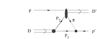
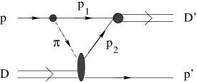
(a)                                                      (b)                                         (c)

Figure .1: The one-nucleon (a) and the one-pion exchange graphs (b) and (c) for the reaction $p\,+\,D\,=\,p^{\prime}(\theta^{*}=180^{o})\,+\,D^{\prime}$.

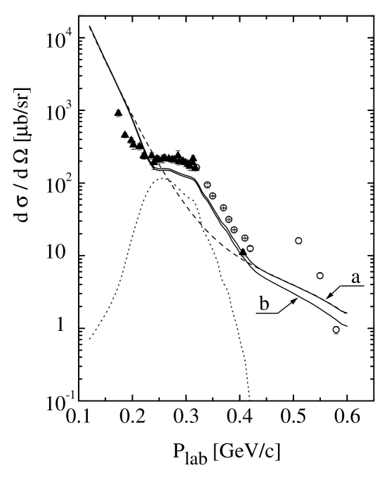
Figure .2: The spin averaged differential cross section $\displaystyle\frac{d\sigma}{d\mathchar 266\relax}$ for the elastic $pD$ backward scattering in the center of mass system as a function of the momentum of the detected proton in the laboratory system. Dashed line: the contribution of the one-nucleon exchange mechanism; dotted line: results of calculations of the triangle diagram; solid line: the full BS calculations with $P$ waves (a), or without $P$ waves (b); The experimental data are from [21, 19].

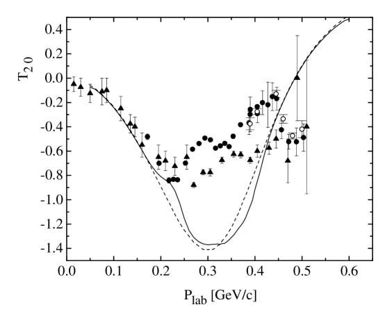
Figure .3: The deuteron tensor analyzing power $T_{20}$ for the elastic $pD$ scattering. Dashed line: the contribution of the one-nucleon exchange mechanism; solid line: the result of computation within the BS approach, including contributions from the triangle diagram. Experimental data: circles - $T_{20}$ for the elastic backward scattering, ref. [7, 8, 12], triangles - $T_{20}$ measured in the deuteron break up reactions [6].

Figure .4: The deuteron to proton polarization transfer $\kappa_{D\to p}$ for the elastic $pD$ backward scattering. Notation as in Fig. 3.

Figure .5: The vector-vector polarization transfer coefficient from the initial proton to the final proton. Dashed line: contribution of the one-nucleon exchange mechanism; solid line: the full BS results.

References

• 1. I.M. Sitnik et al., JINR Rapid Communication 2(70)-95, p. 19, “The measurement of spin correlations in the reaction D+p $\to$ p+D (Proposal)”, Dubna (1995)
• 2. V.I. Komarov (spokesman) et al., COSY proposal #20 “Exclusive deuteron break-up study with polarized protons and deuterons at COSY”,
V.I. Komarov et al., KFA Annual Rep. Jülich (1995) 64,
A.K. Kacharava et al., JINR Communication E1-96-42, Dubna, 1996,
C.F. Perdrisat (spokesperson) et al., COSY proposal #68.1 ”Proton-to-proton polarization transfer in backward elastic scattering”
• 3. E. Tomasi-Gustafsson, “New Information on Nucleon and Deuteron Form Factors through Deuteron Polarization Observables”, Proc. of XIV International Seminar On High Energy Physics Problems Dubna, August 17-22, 1998 (transparencies are available via http://pc7236.jinr.ru/ishepp/tr)
• 4. F. Rotz, H. Arenhövel, T. Wilbois, nucl-th/9707045,
H. Arenhövel, W. Leidemann, L. Tomusiak, Phys. Rev. C52, 1232 (1995), Phys. Rev. C46 455 (1992)
• 5. M.P. Rekalo, N.M. Piskunov, I.M. Sitnik, Few Body Syst. 23, 187 (1998), E4-96-328, Preprint JINR, Dubna, 1996, Russian J. Nucl. Phys. 57, 2089 (1994)
• 6. V.G. Ableev et al., Nucl. Phys. A393, 491 (1983),
C.F. Perdrisat, V. Punjabi, Phys. Rev. C42, 1899 (1990),
B. Kühn, C.F. Perdrisat, E.A. Strokovsky, Phys. Lett. B312, 298 (1994),
A.P. Kobushkin, A.I. Syamtomov, C.F. Perdrisat, V. Punjabi, Phys. Rev. C50, 2627 (1994),
J. Erö et al., Phys. Rev. C50, 2687 (1994),
J. Arvieux et al., Nucl. Phys. A431, 6132 (1984)
• 7. M.P. Rekalo, I.M. Sitnik, Phys. Lett. B356, 434 (1995),
L.S. Azhgirei et al., Phys. Lett. B 361, 21 (1995)
• 8. V. Punjabi et al., Phys. Lett. B350, 178 (1995)
• 9. S.L. Belostotski et al., Phys. Rev. C56, 50 (1997)
• 10. N.P. Aleshin et al., Nucl. Phys. A568, 809 (1994)
• 11. V.P. Ladygin, N.B. Ladygina, J. Phys. G23, 847 (1997),
V.P. Ladygin, Phys. Atom. Nucl., 60, 1238 (1997)
• 12. L.S. Azhgiey et al., Phys. Lett. B391, 22 (1997)
• 13. L.P. Kaptari, B. Kämpfer, S.M. Dorkin, S.S. Semikh, Phys. Rev. C57, 1097 (1998), Phys. Lett. B404, 8 (1997)
• 14. F.D. Santos, A. Arriaga, Phys. Lett. B325, 267 (1994)
• 15. L.S. Kisslinger, in Mesons in Nuclei, (Eds.) M. Rho, D. Wilkinson; North-Holland, Amsterdam, 1978
• 16. B.D. Keister, J.A. Tjon, Phys. Rev. C26, 578 (1982),
B.D. Keister, Phys. Rev. C24, 2628 (1981) 2628
• 17. L.P. Kaptari, A.Yu. Umnikov, F.C. Khanna, B. Kämpfer, Phys. Lett. B351, 400 (1995)
• 18. N.S. Craigie, C. Wilkin, Nucl. Phys. B14, 477 (1969)
• 19. A. Nakamura, L. Satta, Nucl. Phys. A445, 706 (1985)
• 20. V.M. Kolybasov, N.Ya. Smorodinskaya, Phys. Lett. B37, 272 (1971)
• 21. P. Berthet et al., J. Phys. G8, L111 (1982),
L. Dubai et al., Phys. Rev. D9, 597 (1974)
• 22. A.Yu. Umnikov, L.P. Kaptari, F.C Khanna, Phys. Rev. C56, 1700 (1997),
A.Yu. Umnikov, L.P. Kaptari, K.Yu. Kazakov, F.C. Khanna, Phys. Lett. B334, 163 (1994)
• 23. A.Yu. Umnikov, Z. Phys. A357, 333 (1997)
• 24. R.G. Arnold, C.E. Carlson, F. Gross, Phys. Rev. C21, 1426 (1980),
F. Gross, J.W. Van Orden, K. Holinde, Phys. Rev. C45, 2094 (1992) 2094,
F. Gross, Phys. Rev. 186, 1448 (1969) 1448
• 25. L.P. Kaptari, A.Yu. Umnikov, S.G. Bondarenko, K.Yu. Kazakov, F.C. Khanna, B. Kämpfer, Phys. Rev. C54, 986 (1996)
• 26. C. Itzykson, J-B. Zuber, Quantum Field Theory, McGraw-Hill International Editions, Physics Series, Singapore, 1985
• 27. R.A. Arndt, I.I. Strakovsky, R.L. Workman, D.V. Bugg, Phys. Rev. C48, 1926 (1993) 1926,
C.H. Oh, R.A. Arndt, I.I. Strakovsky, R.L. Workman, Phys. Rev. C56, 635 (1997)
• 28. C. Bourrely, E. Leader, J. Soffer, Phys. Rep. 59, 95 (1980)
• 29. J. Fleisher, J.A. Tjon, Nucl. Phys. B84, 375 (1975),
Yu.L. Dorodnych et al., Phys. Rev. C43, 2499 (1991)
Refer to caption
Refer to caption
Refer to caption
(a)                                                      (b)                                         (c)