Survey of heavy-meson observables

Abstract

We employ a Dyson-Schwinger equation model to effect a unified and uniformly accurate description of light- and heavy-meson observables, which we characterise by heavy-meson leptonic decays, semileptonic heavy-to-heavy and heavy-to-light transitions - $B\to D^{\ast}$, $D$, $\rho$, $\pi$; $D\to K^{\ast}$, $K$, $\pi$, radiative and strong decays - $B_{(s)}^{\ast}\to B_{(s)}\gamma$; $D_{(s)}^{*}\to D_{(s)}\gamma$, $D\pi$, and the rare $B\to K^{\ast}\gamma$ flavour-changing neutral-current process. We elucidate the heavy-quark limit of these processes and, using a model-independent mass formula valid for all nonsinglet pseudoscalar mesons, demonstrate that their mass rises linearly with the mass of their heaviest constituent. In our numerical calculations we eschew a heavy-quark expansion and rely instead on the observation that the dressed $c,b$-quark mass functions are well approximated by a constant, interpreted as their constituent-mass: we find $\hat{M}_{c}=1.32\,$GeV and $\hat{M}_{b}=4.65\,$GeV. The calculated heavy-meson leptonic decay constants and transition form factors are a necessary element in the experimental determination of CKM matrix elements. The results also show that this framework, as employed hitherto, is well able to describe vector meson polarisation observables.

I Introduction

Mesons are the simplest bound states in QCD, and their non-hadronic electroweak interactions provide an important tool for exploring their structure and elucidating the nonperturbative, long-distance behaviour of the strong interaction. That elucidation is accomplished most effectively by applying a single framework to a broad range of observables, and in this the bound state phenomenology [1, 2] based on Dyson-Schwinger equations (DSEs) [3] has been successful; e.g., with its simultaneous application to phenomena as diverse as $\pi$-$\pi$ scattering [4, 5], the electromagnetic form factors of light pseudoscalar mesons [6, 7, 8], anomalous pion [4] and photo-pion [8, 9, 10] processes, and the diffractive electroproduction [11] and electromagnetic form factors [12] of vector mesons. Herein we extend this application and implement a simplification valid for heavy quarks, so obtaining in addition a description of heavy-meson observables. We illustrate that by reporting the simultaneous calculation of a range of light-meson observables and heavy-meson leptonic decays, semileptonic heavy-to-heavy and heavy-to-light transitions - $B\to D^{*}$, $D$, $\rho$, $\pi$; $D\to K^{\ast}$, $K$, $\pi$, radiative and strong decays - $B_{(s)}^{\ast}\to B_{(s)}\gamma$; $D_{(s)}^{*}\to D_{(s)}\gamma$, $D\pi$, and the rare $B\to K^{\ast}\gamma$ flavour-changing neutral-current process. This is an extensive but not exhaustive range of applications.

To introduce the heavy-quark simplification we observe that mesons, whether heavy or light, are bound states of a dressed-quark and -antiquark, where the dressing is described by the quark Dyson-Schwinger equation (DSE) [3]:

$$S_{f}(p)^{-1} := i\gamma\cdot p\,A_{f}(p^{2})+B_{f}(p^{2})=A_{f}(p^{2})\left(i\gamma\cdot p+M_{f}(p^{2})\right)$$ (1)

$$= Z_{2}(i\gamma\cdot p+m_{f}^{\rm bm})+\,Z_{1}\,\int^{\Lambda}_{q}\,g^{2}D_{\mu\nu}(p-q)\frac{\lambda^{a}}{2}\gamma_{\mu}S_{f}(q)\Gamma^{fa}_{\nu}(q,p)\,.$$ (2)

Here $f\,(=u,d,s,c,b)$ is a flavour label, $D_{\mu\nu}(k)$ is the dressed-gluon propagator, $\Gamma^{fa}_{\nu}(q,p)$ is the dressed-quark-gluon vertex, $m_{f}^{\rm bm}$ is the $\Lambda$-dependent current-quark bare mass and $\int^{\Lambda}_{q}:=\int^{\Lambda}d^{4}q/(2\pi)^{4}$ represents mnemonically a translationally-invariant regularisation of the integral, with $\Lambda$ the regularisation mass-scale. The renormalisation constants for the quark-gluon-vertex and quark wave function, $Z_{1}(\zeta^{2},\Lambda^{2})$ and $Z_{2}(\zeta^{2},\Lambda^{2})$, depend on the renormalisation point, $\zeta$, and the regularisation mass-scale, as does the mass renormalisation constant $Z_{m}(\zeta^{2},\Lambda^{2}):=Z_{2}(\zeta^{2},\Lambda^{2})^{-1}Z_{4}(\zeta^{2},\Lambda^{2})$. However, one can choose the renormalisation scheme such that they are flavour-independent.

This equation has been much studied and the qualitative features of its solution elucidated. In QCD the chiral limit is defined by $\hat{m}=0$, where $\hat{m}$ is the renormalisation-point-independent current-quark mass. It follows that in this case there is no scalar, mass-like divergence in the perturbative evaluation of the quark self energy. Hence, for $p^{2}>20\,$GeV² the solution of Eq. (2) for the chiral-limit quark mass-function is [13]

$$M_{0}(p^{2})\stackrel{{\scriptstyle{\rm large}-p^{2}}}{{=}}\,\frac{2\pi^{2}\gamma_{m}}{3}\,\frac{\left(-\,\langle\bar{q}q\rangle^{0}\right)}{p^{2}\left(\frac{1}{2}\ln\left[p^{2}/\Lambda_{\rm QCD}^{2}\right]\right)^{1-\gamma_{m}}}\,,$$ (3)

where $\gamma_{m}=12/(33-2N_{f})$ is the gauge-independent mass anomalous dimension and $\langle\bar{q}q\rangle^{0}$ is the renormalisation-point-independent vacuum quark condensate. The existence of dynamical chiral symmetry breaking (DCSB) means that $\langle\bar{q}q\rangle^{0}\neq 0$, however, its actual value depends on the long-range behaviour of $D_{\mu\nu}(k)$ and $\Gamma^{0a}_{\nu}(q,p)$, which is modelled in contemporary DSE studies. $\langle\bar{q}q\rangle^{0}\approx-(0.24\,\mbox{GeV})^{3}$ is consistent with light-meson observables [14].

In contrast, for $\hat{m}_{f}\neq 0$,

$$M_{f}(p^{2})\stackrel{{\scriptstyle{\rm large}-p^{2}}}{{=}}\frac{\hat{m}_{f}}{\left(\frac{1}{2}\ln\left[p^{2}/\Lambda_{\rm QCD}^{2}\right]\right)^{\gamma_{m}}}\,.$$ (4)

An obvious qualitative difference is that, relative to Eq. (4), the chiral-limit solution is $1/p^{2}$-suppressed in the ultraviolet.

There is some quantitative model-dependence in the momentum-evolution of the mass-function into the infrared. However, for any forms of $D_{\mu\nu}(k)$ and $\Gamma^{fa}_{\nu}(q,p)$ that provide an accurate description of $f_{\pi,K}$ and $m_{\pi,K}$, one obtains [15] quark mass-functions with profiles like those illustrated in Fig. 1. The evolution to coincidence between the chiral-limit and $u,d$-quark mass functions, apparent in this figure, makes clear the transition from the perturbative to the nonperturbative domain. The chiral limit mass-function is nonzero only because of the nonperturbative DCSB mechanism whereas the $u,d$-quark mass function is purely perturbative at $p^{2}>20\,$GeV², where Eq. (4) is accurate. The DCSB mechanism thus has a significant effect on the propagation characteristics of $u,d,s$-quarks.

However, as evident in the figure, that is not the case for the $b$-quark. Its large current-quark mass almost entirely suppresses momentum-dependent dressing, so that $M_{b}(p^{2})$ is nearly constant on a substantial domain. This is true to a lesser extent for the $c$-quark.

We employ ${\cal L}_{f}:=M^{E}_{f}/m_{f}^{\zeta}$ as a single, quantitative measure of the importance of the DCSB mechanism; i.e., nonperturbative effects, in modifying the propagation characteristics of a given quark flavour. In this particular illustration it takes the values:

$$\begin{array}[]{c|ccccc}f&u,d&s&c&b\\ \hline\cr{\cal L}_{f}&150&10&2.2&1.2\end{array}\,.$$ (5)

These values are representative: for light-quarks ${\cal L}_{q=u,d,s}\sim 10$-$100$, while for heavy-quarks ${\cal L}_{Q=c,b}\sim 1$, and highlight the existence of a mass-scale characteristic of DCSB: $M_{\chi}$. The propagation characteristics of a flavour with $m_{f}^{\zeta}\leq M_{\chi}$ are significantly altered by the DCSB mechanism, while for flavours with $m_{f}^{\zeta}\gg M_{\chi}$ momentum-dependent dressing is almost irrelevant. It is apparent and unsurprising that $M_{\chi}\sim 0.2\,$GeV$\,\sim\Lambda_{\rm QCD}$. As a consequence we anticipate that the propagation of $c,b$-quarks can be described well by replacing their mass-functions with a constant; i.e., writing

$$S_{Q}(p)=\frac{1}{i\gamma\cdot p+\hat{M}_{Q}}\,,\;Q=c,b\,,$$ (6)

where $\hat{M}_{Q}$ is a constituent-heavy-quark mass parameter. We expect that a good description of observable phenomena will require $\hat{M}_{Q}\approx M_{Q}^{E}$.

When considering a meson with a heavy-quark constituent one can proceed further, as in heavy-quark effective theory (HQET) [17], allow the heaviest quark to carry all the heavy-meson momentum:

$$P_{\mu}=:m_{H}v_{\mu}=:(\hat{M}_{Q}+E_{H})v_{\mu},$$ (7)

and write

$$S_{Q}(k+P)=\frac{1}{2}\,\frac{1-i\gamma\cdot v}{k\cdot v-E_{H}}+{\rm O}\left(\frac{|k|}{\hat{M}_{Q}},\frac{E_{H}}{\hat{M}_{Q}}\right)\,,$$ (8)

where $k$ is the momentum of the lighter constituent. In the calculation of observables, the meson’s Bethe-Salpeter amplitude will limit the range of $|k|$ so that Eq. (8) will only be a good approximation if both the momentum-space width of the amplitude, $\omega_{H}$, and the binding energy, $E_{H}$, are significantly less than $\hat{M}_{Q}$.

In Ref. [18] the propagation of $c$- and $b$-quarks was described by Eq. (8), with a goal of exploring the fidelity of that idealisation. It was found to allow for a uniformly good description of $B_{f}$-meson leptonic and semileptonic decays with heavy- and light-pseudoscalar final states. In that study, corrected as described below, $\omega_{B_{f}}\approx 1.3\,$GeV and $E_{B_{f}}\approx 0.70\,$GeV, both of which are small compared with $\hat{M}_{b}\approx 4.6\,$GeV in Fig. 1, so that the accuracy of the approximation could be anticipated. It is reasonable to expect that $\omega_{D}\approx\omega_{B}$ and $E_{D}\approx E_{B}$, since they must be the same in the limit of exact heavy-quark symmetry. Hence in processes involving the weak decay of a $c$-quark ($\hat{M}_{c}\approx 1.3\,$GeV) where a $D_{f}$-meson is the heaviest participant, Eq. (8) must be inadequate; an expectation verified in Ref. [18].

The failure of Eq. (8) for the $c$-quark complicates or precludes the development of a unified understanding of $D_{f}$- and $B_{f}$-meson observables using such contemporary theoretical tools as HQET and light cone sum rules (LCSRs) [19]. However, the constituent-like dressed-heavy-quark propagator of Eq. (6) can still be used to effect a unified and accurate simplification of the study of these observables. Herein, to demonstrate this, we extend Refs. [18, 22] and employ Eq. (6), with $\hat{M}_{Q}$ treated as free parameters, and parametrisations [6, 7, 8, 9, 11, 12] of the dressed-light-quark propagators and meson Bethe-Salpeter amplitudes in the calculation of a wide range of observables, determining the parameters in a $\chi^{2}$-fit to a subset of them. It is an efficacious strategy.

Our article is divided into eight sections with a single appendix. We discuss heavy- and light-meson leptonic decays in Sec. II, and their masses in Sec. III. In Sec. IV we introduce the impulse approximation to the semileptonic decays of heavy-mesons, and describe the light-quark propagators and meson Bethe-Salpeter amplitudes necessary for their evaluation. The impulse approximation to the other processes is presented in Sec. V, while in Sec. VI we elucidate the heavy-quark symmetry limits of all the decays and transitions. The accuracy of these heavy-quark symmetry predictions is discussed in conjunction with the complete presentation of our results in Sec. VII and Sec. VIII contains some concluding remarks.

II Leptonic Decays

A Pseudoscalar Mesons

The leptonic decay of a pseudoscalar meson, $P(p)$, is described by the matrix element [13]

$$f_{P}\,p_{\mu}:=\langle 0|\bar{\cal Q}\,(T^{P})^{\rm T}\gamma_{\mu}\gamma_{5}\,{\cal Q}|P(p)\rangle={\rm tr}\,Z_{2}\int^{\Lambda}_{k}\,(T^{P})^{\rm T}\gamma_{5}\gamma_{\mu}\,\chi_{P}(k;p),$$ (9)

where $\chi_{P}(k;p)={\cal S}(k+p)\,\Gamma_{P}(k;p)\,{\cal S}(k)$, ${\cal Q}={\rm column}(u,d,s,c,b)$, $T^{P}$ is a flavour matrix identifying the meson; e.g., $T^{\pi^{+}}=\frac{1}{2}\left(\lambda^{1}+i\lambda^{2}\right)$, $(T^{P})^{\rm T}$ is its transpose, ${\cal S}={\rm diag}(S_{u},S_{d},S_{s},S_{c},S_{b})$, and the trace is over colour, Dirac and flavour indices. $\Gamma_{P}$ is the meson’s Bethe-Salpeter amplitude, which is normalised canonically according to:

$$2\,p_{\mu}={\rm tr}\int^{\Lambda}_{q}\,\bar{\Gamma}_{P}(q;-p)\,\frac{\partial{\cal S}(q+p)}{\!\!\!\!\!\!\!\!\!\!\!\!\partial p_{\mu}}\,\Gamma_{P}(q;p)\,{\cal S}(q)$$ (11)

$$+\int^{\Lambda}_{q}\int^{\Lambda}_{k}\,[\bar{\chi}_{P}(q;-p)]_{sr}\frac{\partial K^{rs}_{tu}(q,k;p)}{\!\!\!\!\!\!\!\!\!\!\!\!\partial p_{\mu}}\,[\chi_{P}(k;p)]_{ut}\,,$$

where: $\bar{\Gamma}_{P}^{\rm T}(k,-p)=C^{-1}\Gamma_{P}(-k,-p)C$, with $C=\gamma_{2}\gamma_{4}$, the charge conjugation matrix; $r,s,t,u$ are colour-, Dirac- and flavour-matrix indices; and $K$ is the quark-antiquark scattering kernel. Equation (9) is exact in QCD: the $\Lambda$-dependence of $Z_{2}$ ensures that the right-hand-side (r.h.s.) is finite as $\Lambda\to\infty$, and its $\zeta$- and gauge-dependence is just that necessary to compensate that of $\chi_{P}(k;p)$.

The leptonic decay constants of light pseudoscalar mesons, $\pi$, $K$, are known [20]: $f_{\pi}=0.131\,$GeV, $f_{K}=0.160\,$GeV. The increase with increasing current-quark mass is easily reproduced in DSE studies [13] and continues until at least $3\,\hat{m}_{s}$ [21], at which point the renormalisation-group-improved and confining ladder-like truncation of $K$ used in those studies becomes inadequate, and that model no longer allows the $m_{P}$-dependence of $f_{P}$ to be tracked directly. However, we note from Eq. (11) that

$${\cal G}_{P}(k;p):=\frac{1}{\surd m_{P}}\,\Gamma_{P}(k;p)<\infty\,,m_{P}\to\infty\,;$$ (12)

i.e., that ${\cal G}_{P}(k;p)$ is mass-independent in the heavy-quark symmetry limit, and hence it follows [22] from the general form of the meson Bethe-Salpeter amplitude and Eqs. (8) - (11) that for large pseudoscalar meson masses

$$f_{P}\propto 1/\surd{m_{P}}\,.$$ (13)

In this model-independent result we recover a well-known general consequence of heavy-quark symmetry [17]. However, the value of the current-quark mass at which it becomes evident is unknown in spite of the many studies that report values of $f_{D}$ and $f_{B}$, some of which are tabulated in Ref. [23], and the results of lattice simulations, a summary [24] of which reports

$$f_{D}=200\pm 30\,{\rm MeV}\,,\;f_{B}=170\pm 35\,{\rm MeV}\,.$$ (14)

In Fig. 2 we illustrate the behaviour of $f_{P}$ we anticipate based on these observations. It suggests that D-mesons lie outside the domain on which Eq. (13) is manifest.

B Vector Mesons

The leptonic decay of a vector meson, $V_{\lambda}(p)$, is described by the matrix element ($\epsilon_{\mu}^{\lambda}(p)$ is the polarisation vector: $\epsilon^{\lambda}(p)\cdot p=0$)

$$f_{V}\,M_{V}\,\epsilon^{\lambda}_{\mu}(p):=\langle 0|\bar{\cal Q}\,(T^{P})^{\rm T}\gamma_{\mu}\,{\cal Q}|V_{\lambda}(p)\rangle\,,$$ (16)

$$\Rightarrow\,f_{V}\,M_{V}=\frac{1}{3}\,{\rm tr}\,Z_{2}\int^{\Lambda}_{k}\,(T^{P})^{\rm T}\gamma_{\mu}\,\chi^{V}_{\mu}(k;p)\,,$$

where $\chi^{V}_{\mu}(k;p)={\cal S}(k+p)\,\Gamma^{V}_{\mu}(k;p)\,{\cal S}(k)$ with $\Gamma^{V}_{\mu}(k;p)$ the vector meson Bethe-Salpeter amplitude, which is transverse:

$$p_{\mu}\,\Gamma^{V}_{\mu}(k;p)=0\,,\;p^{2}=-M_{V}^{2}\,,$$ (17)

and normalised according to

$$2\,p_{\mu}=\frac{1}{3}\,{\rm tr}\int^{\Lambda}_{q}\,\bar{\Gamma}^{V}_{\nu}(q;-p)\,\frac{\partial{\cal S}(q+p)}{\!\!\!\!\!\!\!\!\!\!\!\!\partial p_{\mu}}\,\Gamma^{V}_{\nu}(q;p)\,{\cal S}(q)$$ (19)

$$+\int^{\Lambda}_{q}\int^{\Lambda}_{k}\,[\bar{\chi}^{V}_{\nu}(q;-p)]_{sr}\frac{\partial K^{rs}_{tu}(q,k;p)}{\!\!\!\!\!\!\!\!\!\!\!\!\partial p_{\mu}}\,[\chi^{V}_{\nu}(k;p)]_{ut}\,,$$

an analogue of Eq. (11). The obvious analogue of Eq. (12) is true.

Such decays are difficult to observe directly but it is possible to estimate $f_{\rho}$ and hence identify the natural scale of $f_{V}$. In the isospin-symmetric limit the $\rho^{0}\to e^{+}e^{-}$ decay constant, $g_{\rho}$, is obtained from the matrix element

$$\frac{M_{\rho}^{2}}{g_{\rho}}\,\epsilon^{\lambda}_{\mu}(p):=\langle 0|\bar{u}\gamma_{\mu}u|\rho^{0}_{\lambda}(p)\rangle=\frac{1}{\surd 2}\,\langle 0|\bar{u}\gamma_{\mu}d|\rho^{-}_{\lambda}(p)\rangle$$ (20)

so that

$$f_{\rho}=\surd 2\,\frac{M_{\rho}}{g_{\rho}}\,.$$ (21)

The experimentally measured width [20] $\Gamma_{\rho^{0}\to e^{+}e^{-}}=6.77\pm 0.32\,$keV yields $g_{\rho}=5.03\pm 0.12$ and hence

$$f_{\rho}=216\pm 5\,{\rm MeV}\,.$$ (22)

For the vector-mesons it follows from the general form of the Bethe-Salpeter amplitude, and Eqs. (8), (16) and (19) that for large vector-meson masses

$$f_{V}\propto 1/\surd{M_{V}}\,,$$ (23)

which again is a model-independent and general consequence of heavy-quark symmetry. In fact, as we illustrate below,

$$f_{P}=f_{V}\propto 1/\surd\hat{m}_{Q}\,,\;\hat{m}_{Q}\to\infty\,;$$ (24)

i.e., observables are spin-independent in the heavy-quark symmetry limit [17].

III Pseudoscalar Meson Masses

Flavour nonsinglet pseudoscalar meson masses satisfy [13]

$$f_{P}\,m_{P}^{2} = {\cal M}_{P}^{\zeta}\,r^{\zeta}_{P}\,,\;{\cal M}_{P}^{\zeta}:={\rm tr}_{\rm flavour}\left[M^{\zeta}\,\left\{T^{P},(T^{P})^{\rm T}\right\}\right]\,,$$ (25)

with $M^{\zeta}={\rm diag}(m_{u}^{\zeta},m_{d}^{\zeta},m_{s}^{\zeta},m_{c}^{\zeta},m_{b}^{\zeta})$ and

$$i\,r_{P}^{\zeta} = {\rm tr}\,Z_{4}\int^{\Lambda}_{k}\,\left(T^{P}\right)^{\rm T}\gamma_{5}\,\chi_{P}(k;p)\,.$$ (26)

The renormalisation constant, $Z_{4}$, ensures that $r_{P}^{\zeta}$ is finite as $\Lambda\to\infty$, and its $\zeta$- and gauge-dependence is just that necessary to ensure that the product on the r.h.s. of Eq. (25) is gauge invariant and renormalisation point independent.

In the limit of small current-quark masses one obtains [13] what is commonly called the Gell-Mann–Oakes–Renner relation as a corollary of Eq. (25); i.e., $m_{P}^{2}\propto\hat{m}_{f}$, $\hat{m}_{f}\to 0$. However, it also has an important corollary in the heavy-quark symmetry limit. Using Eqs. (8) and (12)

$$r_{P}\propto\surd m_{P}\,,\;m_{P}\to\infty\,,$$ (27)

from which Eqs. (13) and (25) yield

$$m_{P}\propto\hat{m}_{Q}\,,\;\hat{m}_{Q}\to\infty\,.$$ (28)

Thus the quadratic trajectory, valid when the current-quark mass of the constituents is small, evolves into a linear trajectory when this mass becomes large. In all phenomenologically efficacious DSE models the linear trajectory is manifest at twice the $s$-quark current-mass [15] so that $m_{K}$ lies on the extrapolation of the straight line joining $m_{D}$ and $m_{B}$ in the $(\hat{m}_{f},m_{P})$-plane [2].

IV Semileptonic Transition Form Factors

A Pseudoscalar meson in the final state

The pseudoscalar$\,\to\,$pseudoscalar transition: $P_{1}(p_{1})\to P_{2}(p_{2})\,\ell\,\nu\,,$ where $P_{1}$ represents either a $B$ or $D$ and $P_{2}$ can be a $D$, $K$ or $\pi$, is described by the invariant amplitude

$$A(P_{1}\to P_{2}\,\ell\,\nu)=\frac{G_{F}}{\surd 2}\,V_{f^{\prime}f}\,\bar{\ell}\,\gamma_{\mu}(1-\gamma_{5})\nu\,M_{\mu}^{P_{1}P_{2}}(p_{1},p_{2})\,,$$ (29)

where $G_{F}=1.166\times 10^{-5}\,$GeV^-2, $V_{f^{\prime}f}$ is the relevant element of the Cabibbo-Kobayashi-Maskawa (CKM) matrix, and the hadronic current is

$$M_{\mu}^{P_{1}P_{2}}(p_{1},p_{2}) := \langle P_{2}(p_{2})|\bar{f}^{\prime}\gamma_{\mu}f|P_{1}(p_{1})\rangle=f_{+}(t)(p_{1}+p_{2})_{\mu}+f_{-}(t)q_{\mu}\,,$$ (30)

with $t:=-q^{2}=-(p_{1}-p_{2})^{2}$. The transition form factors, $f_{\pm}(t)$, contain all the information about strong-interaction effects in these processes, and their accurate calculation is essential for a reliable determination of the CKM matrix elements from a measurement of the decay width ($t_{\pm}:=(m_{P_{1}}\pm m_{P_{2}})^{2}$):

$$\Gamma(P_{1}\to P_{2}\ell\nu)=\frac{G_{F}^{2}}{192\pi^{3}}\,|V_{f^{\prime}f}|^{2}\,\frac{1}{m_{P_{1}}^{3}}\,\int_{0}^{t_{-}}\,dt\,|f_{+}(t)|^{2}\,\left[(t_{+}-t)(t_{-}-t)\right]^{3/2}\!\!.$$ (31)

B Vector meson in the final state

The pseudoscalar$\,\to\,$vector transition: $P(p_{1})\to V_{\lambda}(p_{2})\,\ell\,\nu\,,$ with $P$ either a $B$ or $D$ and $V_{\lambda}$ a $D^{\ast}$, $K^{\ast}$ or $\rho$, is described by the invariant amplitude

$$A(P\to V_{\lambda}\,\ell\,\nu)=\frac{G_{F}}{\surd 2}\,V_{f^{\prime}f}\,\bar{\ell}\,i\gamma_{\mu}(1-\gamma_{5})\nu\,\epsilon_{\nu}^{\lambda}(p_{2})\,M_{\mu\nu}^{PV_{\lambda}}(p_{1},p_{2})\,,$$ (32)

where the hadronic tensor involves four scalar functions

$$\epsilon_{\nu}^{\lambda}(p_{2})\,M_{\mu\nu}^{PV_{\lambda}}(p_{1},p_{2})=$$ (35)

$$\epsilon_{\mu}^{\lambda}\,(m_{P}+M_{V})\,A_{1}(t)+(p_{1}+p_{2})_{\mu}\,\epsilon^{\lambda}\cdot q\,\frac{A_{2}(t)}{m_{P}+M_{V}}$$

$$+\,q_{\mu}\,\epsilon^{\lambda}\cdot q\,\frac{A_{3}(t)}{m_{P}+M_{V}}\,+\,\varepsilon_{\mu\nu\alpha\beta}\,\epsilon_{\nu}^{\lambda}\,p_{1\alpha}\,p_{2\beta}\,\frac{2V(t)}{m_{P}+M_{V}}\,.$$

The contribution of $A_{3}$ can be neglected unless $\ell=\tau$.

Introducing three helicity amplitudes

$$H_{\pm}=(m_{P}+M_{V})\,A_{1}(t)\,\mp\,\frac{\lambda^{\frac{1}{2}}(m_{P}^{2},M_{V}^{2},t)}{m_{P}+M_{V}}\,V(t)\,,$$ (36)

$$H_{0}=$$ (38)

$$\!\!\!\!\frac{1}{2\,M_{V}\,\surd t}\left(\left[m_{P}^{2}-M_{V}^{2}-t\right]\,\left[m_{P}+M_{V}\right]A_{1}(t)-\frac{\lambda(m_{P}^{2},M_{V}^{2},t)}{m_{P}+M_{V}}\,A_{2}(t)\right)\!,$$

where $\lambda(m_{P}^{2},M_{V}^{2},t)=[t_{+}-t]\,[t_{-}-t]$, $t_{\pm}=(m_{P}\pm M_{V})^{2}$, the transition rates can be expressed as

$$\frac{d\Gamma_{\pm,0}}{dt} = \frac{G_{F}^{2}}{192\pi^{3}m_{P_{1}}^{3}}\,|V_{f^{\prime}f}|^{2}\,t\,\lambda^{\frac{1}{2}}(m_{P}^{2},M_{V}^{2},t)\,|H_{\pm,0}(t)|^{2}\,,$$ (39)

and the transverse and longitudinal rates and widths are

$$\frac{d\Gamma_{T}}{dt} = \frac{d\Gamma_{+}}{dt}+\frac{d\Gamma_{-}}{dt}\,,\;\Gamma_{T}=\int_{0}^{t_{-}}\,dt\,\frac{d\Gamma_{T}}{dt}\,,$$ (40)

$$\frac{d\Gamma_{L}}{dt} = \frac{d\Gamma_{0}}{dt}\,,\;\Gamma_{L}=\int_{0}^{t_{-}}\,dt\,\frac{d\Gamma_{L}}{dt}\,,$$ (41)

with the total width: $\Gamma=\Gamma_{T}+\Gamma_{L}$. The polarisation ratio and forward-backward asymmetry are

$$\alpha=2\,\frac{\Gamma_{L}}{\Gamma_{T}}-1\,, A_{\rm FB}=\frac{3}{4}\,\frac{\Gamma_{-}-\Gamma_{+}}{\Gamma}\,.$$ (42)

C Impulse Approximation

We employ the impulse approximation in calculating the hadronic contribution to these invariant amplitudes:

$${\cal H}^{PX}_{\mu}(p_{1},p_{2})=$$ (44)

$$2N_{c}\,{\rm tr}_{D}\,\int_{k}^{\Lambda}\,\bar{\Gamma}_{X}(k;-p_{2})\,S_{q}(k_{2})\,i{\cal O}_{\mu}^{qQ}(k_{2},k_{1})\,S_{Q}(k_{1})\,\Gamma_{P}(k;p_{1})\,S_{q^{\prime}}(k),$$

where the flavour structure has been made explicit, $k_{1,2}=k+p_{1,2}$ and:

$${\cal H}^{P_{1}X=P_{2}}_{\mu}(p_{1},p_{2}) = M_{\mu}^{P_{1}P_{2}}(p_{1},p_{2})\,,$$ (45)

$${\cal H}^{PX=V^{\lambda}}_{\mu}(p_{1},p_{2}) = \epsilon_{\nu}^{\lambda}(p_{2})\,M_{\mu\nu}^{PV_{\lambda}}(p_{1},p_{2})\,;$$ (46)

$\Gamma_{X=V^{\lambda}}(k;p)=\epsilon^{\lambda}(p)\cdot\Gamma^{V}(k;p)$; and ${\cal O}_{\mu}^{qQ}(k_{2},k_{1})$ is the dressed-quark-W-boson vertex, which in weak decays of heavy-quarks is well approximated [18, 22] by

$${\cal O}_{\mu}^{qQ}(k_{2},k_{1})=\gamma_{\mu}\,(1-\gamma_{5})\,.$$ (47)

The impulse approximation has been used widely and efficaciously in phenomenological DSE studies; e.g., Refs. [6, 7, 8, 9, 10, 11, 12, 18, 22]. It is self-consistent only if the quark-antiquark scattering kernel is independent of the total momentum. Corrections can be incorporated systematically [26] and their effect in processes such as those considered herein has been estimated [27, 28]: they vanish with increasing spacelike momentum transfer and contribute $\mathrel{\hbox to0.0pt{\lower 4.0pt\hbox{\hskip 0.0pt$\sim$}\hss}\raise 1.0pt\hbox{$<$}}15$% even at the extreme kinematic limit, $t=t_{-}$.

D Quark Propagators

To evaluate ${\cal H}^{P_{1}X}_{\mu}(p_{1},p_{2})$ a specific form for the dressed-quark propagators is required. As argued in Sec. I, Eq.(6) provides a good approximation for the heavier quarks, $Q=c,b$, and we use that herein with $\hat{M}_{Q}$ treated as free parameters. For the light-quark propagators:

$$S_{f}(p)=-i\gamma\cdot p\,\sigma^{f}_{V}(p^{2})+\sigma^{f}_{S}(p^{2})=\frac{1}{i\gamma\cdot p\,A_{f}(p^{2})+B_{f}(p^{2})}\,,$$ (48)

$f=u,s$ (isospin symmetry is assumed), we use the algebraic forms introduced in Ref. [6], which efficiently characterise the essential and robust elements of the solution of Eq. (2) and have been used efficaciously in Refs. [6, 7, 8, 9, 11, 12, 18, 22]:

$$\bar{\sigma}^{f}_{S}(x) = 2\bar{m}_{f}{\cal F}(2(x+\bar{m}_{f}^{2}))+{\cal F}(b_{1}x){\cal F}(b_{3}x)\left(b^{f}_{0}+b^{f}_{2}{\cal F}(\epsilon x)\right)\,,$$ (49)

$$\bar{\sigma}^{f}_{V}(x) = \frac{2(x+\bar{m}_{f}^{2})-1+e^{-2(x+\bar{m}_{f}^{2})}}{2(x+\bar{m}_{f}^{2})^{2}}\,,$$ (50)

${\cal F}(y)=(1-{\rm e}^{-y})/y$, $x=p^{2}/\lambda^{2}$; $\bar{m}_{f}$ = $m_{f}/\lambda$; and

$$\bar{\sigma}_{S}^{f}(x)=\lambda\,\sigma_{S}^{f}(p^{2})\,, \bar{\sigma}_{V}^{f}(x)=\lambda^{2}\,\sigma_{V}^{f}(p^{2})\,,$$ (51)

with $\lambda$ a mass scale. This algebraic form combines the effects of confinement and DCSB with free-particle behaviour at large, spacelike $p^{2}$.

The chiral limit vacuum quark condensate is [13]

$$-\langle\bar{q}q\rangle^{0}_{\zeta} := \lim_{\Lambda^{2}\to\infty}\,N_{c}\,{\rm tr}_{D}\,Z_{4}(\zeta^{2},\Lambda^{2})\,\int_{k}^{\Lambda}\,S_{0}(k),$$ (52)

where at one-loop order $Z_{4}(\zeta^{2},\Lambda^{2})=[\alpha(\Lambda^{2})/\alpha(\zeta^{2})]^{\gamma_{m}(1+\xi/3)}$, with $\xi$ the covariant-gauge parameter ($\xi=0$ specifies Landau gauge). The $\xi$-dependence of $Z_{4}(\zeta^{2},\Lambda^{2})$ is just that required to ensure that $\langle\bar{q}q\rangle^{0}_{\zeta}$ is gauge independent. The parametrisation of Eq. (49) provides a model that corresponds to the replacement $\gamma_{m}\to 1$ in Landau gauge, in which case, with $S_{0}:=S_{u,m=0}$, Eq. (52) yields

$$-\langle\bar{u}u\rangle_{\zeta} = \lambda^{3}\,\frac{3}{4\pi^{2}}\,\frac{b_{0}^{u}}{b_{1}^{u}\,b_{3}^{u}}\,\ln\frac{\zeta^{2}}{\Lambda_{\rm QCD}^{2}}\,.$$ (53)

This is a signature of DCSB in the model.

In Ref. [18] the parameters $\bar{m}_{f}$, $b_{0\ldots 3}^{f}$ in Eqs. (49) and (50) take the values

$$\begin{array}[]{c|lllll}&\;\bar{m}_{f}&b_{0}^{f}&b_{1}^{f}&b_{2}^{f}&b_{3}^{f}\\ \hline\cr u&\;0.00897&0.131&2.90&0.603&0.185\\ s&\;0.224&0.105&2.90&0.740&0.185\end{array}$$ (54)

with $\lambda=0.566\,$GeV, which were determined [7] in a least-squares fit to a range of light-hadron observables, and we note that with $\Lambda_{\rm QCD}=0.2\,$GeV they yield $\langle\bar{u}u\rangle_{1\,{\rm GeV}^{2}}=(-0.22\,{\rm GeV})^{3}$ and $\langle\bar{s}s\rangle_{1\,{\rm GeV}^{2}}=0.8\,\langle\bar{u}u\rangle_{1\,{\rm GeV}^{2}}$. Herein we reconsider this parametrisation and allow $m_{u,s}$, $b_{1}^{u,s}$ and $b_{2}^{u,s}$ to vary. This is a reasonable step provided that in re-fitting to an increased sample of observables the light-quark propagators are pointwise little changed.

E Bethe-Salpeter amplitudes

1 Light Pseudoscalar Mesons

The light-meson Bethe-Salpeter amplitudes can be determined reliably by solving the Bethe-Salpeter equation (BSE) in a truncation consistent with that employed in the quark DSE [13]. However, since for the light-quarks we have parametrised the solution of the quark DSE, we follow Refs. [5, 6, 7, 8, 9, 11, 12, 18, 22] and do the same for the light-meson amplitude; i.e., for the $\pi$- and $K$-mesons we employ $\Gamma_{\pi,K}(k;P)=i\gamma_{5}\,{\cal E}_{\pi,K}(k^{2})$ with,

$${\cal E}_{P}(k^{2})=\frac{1}{\hat{f}_{P}}\,B_{P}(k^{2})\,,\;P=\pi,K\,,$$ (55)

$\hat{f}_{\pi}=f_{\pi}/\surd 2$, where $B_{P}:=\left.B_{u}\right|_{b_{0}^{u}\to b_{0}^{P}}$, obtained from Eq. (48), and $b_{0}^{\pi,K}$ are allowed to vary. This Ansatz follows from the constraints imposed by the axial-vector Ward-Takahashi identity and, together with Eqs. (49) and (50), provides an algebraic representation of $\chi_{P}(k;p)$ valid for small to intermediate meson energy [8, 18].

With this representation, Eqs. (25) and (26) yield the following expression for the $\pi$- and $K$-meson masses:

$$\hat{f}_{P}^{2}\,m_{P}^{2}=-(m_{u}+m_{f^{P}})\,\langle\bar{q}q\rangle_{P}^{1\,{\rm GeV}^{2}}\,,$$ (56)

where $m_{f^{\pi}}=m_{d}$, $m_{f^{K}}=m_{s}$, and the “in-meson condensate” is

$$\langle\bar{q}q\rangle_{P}^{1\,{\rm GeV}^{2}}=-\,\lambda^{3}\,\ln\frac{1}{\Lambda_{\rm QCD}^{2}}\,\frac{3}{4\pi^{2}}\,\frac{b_{0}^{P}}{b_{1}^{u}\,b_{3}^{u}}\,,\;P=\pi,K\,,$$ (57)

and takes typical values [13] $\langle\bar{q}q\rangle_{\pi}^{1\,{\rm GeV}^{2}}=1.05\,\langle\bar{u}u\rangle_{1\,{\rm GeV}^{2}}$ and $\langle\bar{q}q\rangle_{K}^{1\,{\rm GeV}^{2}}=1.64\,\langle\bar{u}u\rangle_{1\,{\rm GeV}^{2}}$.

2 Light Vector Mesons

The application of DSE-based phenomenology to processes involving vector mesons is less extensive than that involving pseudoscalars. Therefore the modelling of vector meson Bethe-Salpeter amplitudes is less sophisticated. Solutions of a mutually consistent truncation of the quark DSE and meson BSE; e.g., Ref. [29], indicate that a given vector meson is narrower in momentum space than its pseudoscalar partner but that for both vector and pseudoscalar mesons this width increases with the total current-mass of the constituents. These observations are confirmed in calculations of vector meson electroproduction cross sections [11] and electromagnetic form factors [12]. The simple Ansatz

$$\Gamma^{V}_{\mu}(k;p)=\frac{1}{{\cal N}^{V}}\,\left(\gamma_{\mu}+p_{\mu}\,\frac{\gamma\cdot p}{M_{V}^{2}}\right)\,\varphi(k^{2})\,,$$ (58)

where $\varphi(k^{2})=1/(1+k^{4}/\omega_{V}^{4})$ with $\omega_{V}$ a parameter and ${\cal N}^{V}$ fixed by Eq. (19), allows for the realisation of these qualitative features and, from Ref. [12], we expect $\omega_{K^{\ast}}\approx 1.6\,\omega_{\rho}$.

3 Heavy Mesons

Renormalisation-group-improved ladder-like truncations of $K$ employed, e.g., in Refs. [13], are inadequate for heavy-mesons; one reason being that they do not yield the Dirac equation when the mass of one of the fermions becomes large. While an improved truncation valid in this regime is being sought, there is currently no satisfactory alternative and the ladder-like truncations have been used in spite of their inadequacy [29, 30]. Such studies cannot yield a complete and quantitatively reliable spectrum, however, the result that heavy mesons are described by an amplitude whose width behaves as described in Sec. IV E 2 must be qualitatively robust. We therefore use a simple model for the amplitudes that allows a representation of this feature: Eq. (58) for heavy vector mesons, with $\varphi(k^{2})\to\varphi_{H}(k^{2})$, and its analogue for heavy pseudoscalar mesons

$$\Gamma_{P}(k;p)=\frac{1}{{\cal N}^{P}}\,i\,\gamma_{5}\,\varphi_{H}(k^{2})\,,$$ (59)

where $\varphi_{H}(k^{2})=\exp\left(-k^{2}/\omega_{H}^{2}\right)$ and the normalisation is fixed by Eq. (11). We assume the widths are spin and flavour independent; i.e., $\omega_{B}=\omega_{B^{\ast}}=\omega_{B_{s}}$, etc., as would be the case in the limit of exact heavy-quark symmetry, which is a useful but not necessary simplification.

V Other Decay Processes

A Radiative Decays

The radiative decays: $H^{\ast}(p_{1})\to H(p_{2})\,\gamma(k)\,,$ where $H=D_{(s)}$, $B_{(s)}$, are described by the invariant amplitude

$$A(H^{\ast}\to H\,\gamma)=\epsilon_{\mu}^{\lambda_{H}}(p_{1})\,\epsilon_{\nu}^{\lambda_{\gamma}}(k)\left[e_{Q}\,M_{\mu\nu}^{Q}(p_{1},p_{2})+e_{q}\,M_{\mu\nu}^{q}(p_{1},p_{2})\,\right]$$ (60)

$$= \varepsilon_{\mu\nu\alpha\beta}\,\epsilon_{\mu}^{\lambda_{H}}(p_{1})\,\epsilon_{\nu}^{\lambda_{\gamma}}(k)\,p_{1\alpha}\,k_{\beta}\left[e_{Q}\,J^{Q}(t)+e_{q}\,J^{q}(t)\right]\,,$$ (61)

where $t=-k^{2}=-(p_{1}-p_{2})^{2}=0$ and $e_{f}$ is the fractional charge of the active quark in units of the positron charge. The sum indicates that the decay occurs via a spin-flip transition by either the heavy or light quark. The width is

$$\Gamma_{H^{\ast}\to H\gamma}=\frac{\alpha_{\rm em}}{24M_{H^{\ast}}^{3}}\,\lambda^{3/2}(M_{H^{\ast}}^{2},m_{H}^{2},0)\,\left[e_{Q}\,J^{Q}(0)+e_{q}\,J^{q}(0)\right]^{2}\,.$$ (62)

In impulse approximation the hadronic tensors in Eq. (60) are:

$${\cal M}^{Q}_{\mu\nu}(p_{1},p_{2})=$$ (64)

$$2N_{c}\,{\rm tr}_{D}\,\int_{\ell}^{\Lambda}\,\bar{\Gamma}_{P}(\ell;-p_{2})\,S_{Q}(\ell_{2})\,i\Gamma_{\nu}^{Q}(\ell_{2},\ell_{1})\,S_{Q}(\ell_{1})\,\Gamma^{V}_{\mu}(\ell;p_{1})\,S_{q}(\ell),$$

$${\cal M}^{q}_{\mu\nu}(p_{1},p_{2})=$$ (66)

$$2N_{c}\,{\rm tr}_{D}\,\int_{\ell}^{\Lambda}\,\bar{\Gamma}_{P}(\ell;-p_{2})\,S_{Q}(\ell_{1})\,\Gamma^{V}_{\mu}(\ell;p_{1})\,S_{q}(\ell)\,i\Gamma_{\nu}^{q}(\ell,\ell+k)\,S_{q}(\ell+k)\,,$$

where $Q=c$ or $b$, $q=u$ or $s$ and $\ell_{1,2}=\ell+p_{1,2}$.

$\Gamma_{\nu}^{f}(\ell_{1},\ell_{2})$ is the dressed-quark-photon vertex, which satisfies the vector Ward-Takahashi identity:

$$(\ell_{1}-\ell_{2})_{\nu}\,i\Gamma^{f}_{\nu}(\ell_{1},\ell_{2})=S_{f}^{-1}(\ell_{1})-S_{f}^{-1}(\ell_{2})\,,$$ (67)

a feature that ensures current conservation [6]. This vertex has been much studied [31] and, although its exact form remains unknown, its qualitatively robust features have been elucidated so that a phenomenologically efficacious Ansatz has emerged [32]:

$$i\Gamma^{f}_{\nu}(\ell_{1},\ell_{2})=$$ (70)

$$i\Sigma_{A}(\ell_{1}^{2},\ell_{2}^{2})\,\gamma_{\mu}+(\ell_{1}+\ell_{2})_{\mu}\,\left[\frac{1}{2}i\gamma\cdot(\ell_{1}+\ell_{2})\,\Delta_{A}(\ell_{1}^{2},\ell_{2}^{2})+\Delta_{B}(\ell_{1}^{2},\ell_{2}^{2})\right]\,;$$

$$\Sigma_{F}(\ell_{1}^{2},\ell_{2}^{2})=\frac{1}{2}\,[F(\ell_{1}^{2})+F(\ell_{2}^{2})]\,,\;\Delta_{F}(\ell_{1}^{2},\ell_{2}^{2})=\frac{F(\ell_{1}^{2})-F(\ell_{2}^{2})}{\ell_{1}^{2}-\ell_{2}^{2}}\,,$$

where $F=A_{f},B_{f}$; i.e., the scalar functions in Eq. (48). A feature of Eq. (70) is that the vertex is completely determined by the dressed-quark propagator. In Landau gauge the quantitative effect of modifications, such as that canvassed in Ref. [33], is small and can be compensated for by small changes in the parameters that characterise a given model study [34]. The structure in Eq. (70) is only important for light-quarks because, using Eq. (6): $A_{Q}\equiv 1$, $B_{Q}\equiv\hat{M}_{Q}$, and hence

$$\Gamma^{Q}_{\nu}(\ell_{1},\ell_{2})=\gamma_{\mu}\,.$$ (71)

B Strong Decays

The process $H^{\ast}(p_{1})\to H(p_{2})\,\pi(q)$, with $p_{1}^{2}=-M_{H^{\ast}}^{2}$, $p_{2}^{2}=-m_{H}^{2}$ and $q^{2}=-m_{\pi}^{2}$, is described by the invariant amplitude

$$A(H^{\ast}\to H\pi)=\epsilon_{\mu}^{\lambda_{H^{\ast}}}(p_{1})\,M_{\mu}^{H^{\ast}H\pi}(p_{1},p_{2}):=\epsilon_{\mu}^{\lambda_{H^{\ast}}}(p_{1})\,p_{2\mu}\,g_{H^{\ast}H\pi}\,.$$ (72)

$g_{H^{\ast}H\pi}$ can be calculated even when the decay is kinematically forbidden, as for $B^{\ast}$, and is sometimes re-expressed via

$$\bar{g}_{H^{\ast}H\pi}:=\frac{f_{\pi}}{2m_{H}}\,g_{H^{\ast}H\pi}\,.$$ (73)

We calculate the coupling using the impulse approximation, Eq. (A2), and this gives the width:

$$\Gamma_{H^{\ast}H\pi}=\frac{g_{H^{\ast}H\pi}^{2}}{192\,\pi\,M_{H^{\ast}}^{5}}\,\lambda^{3/2}(m_{H}^{2},m_{\pi}^{2},M_{H^{\ast}}^{2})\,.$$ (74)

We also consider the analogous decays of light vector mesons: $\rho(P=k_{1}+k_{2})\to\pi(k_{1})\pi(k_{2})$ and $K^{\ast}(P)\to K(k_{1})\pi(k_{2})$. For these processes the hadronic current can be written

$$M_{\mu}^{VP\pi}(k_{1},k_{2}) = (k_{1}-k_{2})_{\mu}\,f^{+}(t)+P_{\mu}\,f^{-}(t)\,,$$ (75)

which we calculate using the impulse approximation, Eq. (A4). The decay constant is

$$g_{VP\pi}=f^{+}(t=M_{V}^{2})\,,$$ (76)

in terms of which the widths are

$$\Gamma_{\rho\pi\pi} = \frac{g_{\rho\pi\pi}^{2}}{48\pi\,M_{\rho}^{5}}\,\lambda^{3/2}(m_{\pi}^{2},m_{\pi}^{2},M_{\rho}^{2})\,,$$ (77)

$$\Gamma_{K^{\ast}(K\pi)} = \frac{g_{K^{\ast}K\pi}^{2}}{64\pi\,M_{K^{\ast}}^{5}}\,\lambda^{3/2}(m_{K}^{2},m_{\pi}^{2},M_{K^{\ast}}^{2})\,.$$ (78)

C Rare Flavour-Changing Neutral-Current Process

The final decay we consider is the rare, flavour-changing neutral current process: $B(p_{1})\to K^{\ast}(p_{2})\gamma(q)$, which proceeds predominantly [35] via the local magnetic penguin operator:

$$Q_{7\gamma}:=\frac{e}{8\pi^{2}}\,\hat{M}_{b}\,F_{\mu\nu}\,\bar{s}\,\sigma_{\mu\nu}(1+\gamma_{5})\,b\,,$$ (79)

where $F_{\mu\nu}$ is the photon’s field strength tensor, and the effective interaction promoting this process, renormalised at a scale $\zeta\sim\hat{M}_{b}$, is

$$H^{\rm eff}=-\frac{G_{F}}{\surd 2}\,V^{\ast}_{ts}V_{tb}\,C_{7}\,Q_{7\gamma}\,,$$ (80)

with $C_{7}(\hat{M}_{b})=-0.299$ and $|V^{\ast}_{ts}V_{tb}|^{2}=(0.95\pm 0.03)\,|V_{cb}|^{2}$. Consequently, the invariant amplitude describing the decay is

$$A(B\to K^{\ast}\gamma) = -\frac{G_{F}}{\surd 2}\,V^{\ast}_{ts}V_{tb}\,C_{7}\,\frac{e\hat{M}_{b}}{4\pi^{2}}\,\epsilon_{\mu}^{\lambda_{\gamma}}(q)\,\epsilon_{\nu}^{\lambda_{K^{\ast}}}(p_{2})\,M_{\mu\nu}^{B\to K^{\ast}\gamma}(p_{1},p_{2})\,,$$ (81)

with, at $q^{2}=0$,

$$\epsilon_{\mu}^{\lambda_{\gamma}}(q)\,M_{\mu\nu}^{B\to K^{\ast}\gamma}(p_{1},p_{2})=$$ (83)

$$\epsilon_{\mu}^{\lambda_{\gamma}}(q)\,g_{BK^{\ast}\gamma}\,\left(\varepsilon_{\mu\nu\alpha\beta}\,p_{1\alpha}\,p_{2\beta}+\delta_{\mu\nu}(m_{B}^{2}-M_{K^{\ast}}^{2})-(p_{1}+p_{2})_{\mu}\,p_{1\nu}\right).$$

We calculate the coupling using the impulse approximation to the hadronic tensor, Eq. (A6), in terms of which the decay width is

$$\Gamma_{B\to K^{\ast}\gamma}=\alpha_{\rm em}(\hat{M}_{b})\,m_{B}^{3}\,\left(1-\frac{M_{K^{\ast}}^{2}}{m_{B}^{2}}\right)^{3}\,\frac{G_{F}^{2}}{32\pi^{4}}\,\hat{M}_{b}^{2}C_{7}^{2}\,|V_{ts}^{\ast}V_{tb}|^{2}\,g_{BK^{\ast}\gamma}^{2}\,.$$ (84)

VI Heavy-Quark Symmetry Limits

With algebraic representations of the dressed-quark propagators and Bethe-Salpeter amplitudes the calculation of all observables is straightforward. In addition, one can obtain simple formulae that express the heavy-quark symmetry limits. We present them here, and in Sec. VII gauge their accuracy and relevance through a comparison with the results of our complete calculations.

A Leptonic Decays

To begin, using Eq. (8), Eqs. (11) and (19) with $K$ assumed $p$-independent in order to effect a consistent impulse approximation, and Eq. (59) with its analogue for the heavy vector mesons, one finds [22]

$$\frac{1}{m_{H}}\,\frac{1}{\kappa_{f}^{2}}:={\cal N}_{P}^{2}={\cal N}_{V}^{2}=$$ (86)

$$\frac{1}{m_{H}}\,\frac{N_{c}}{4\pi^{2}}\,\int_{0}^{\infty}\,du\,\varphi^{2}_{H}(z)\,\left\{\sigma_{S}^{f}(z)+\surd{u}\,\sigma_{V}^{f}(z)\right\}\,,$$

where $z=u-2E_{H}\surd u$, $f$ labels the meson’s lighter quark and in this section all dimensioned quantities are expressed in units of our mass-scale, $\lambda$. This illustrates Eq. (12). Similarly, using this result with Eq. (8) in Eqs. (9) and (16),

$$f_{P}=f_{V}=$$ (88)

$$\frac{1}{\surd m_{H}}\,\kappa_{f}\,\frac{N_{c}}{2\sqrt{2}\pi^{2}}\,\int_{0}^{\infty}\,du\,\left(\surd u-E_{H}\right)\,\varphi_{H}(z)\,\left\{\sigma_{S}^{f}(z)+\frac{1}{2}\surd{u}\,\sigma_{V}^{f}(z)\right\}\,,$$

which is the promised illustration of Eqs. (13), (23) and (24).

B Semileptonic Heavy$\,\to\,$Heavy Transitions

The semileptonic heavy$\,\to\,$ heavy transition form factors acquire a particularly simple form in the heavy-quark symmetry limit. From Eqs. (30) and (44) one obtains [22]:

$$f_{\pm}(t)={\cal T}_{\pm}\,\xi_{f}(w):=\frac{m_{P_{2}}\pm m_{P_{1}}}{2\sqrt{m_{P_{2}}m_{P_{1}}}}\,\xi_{f}(w),$$ (90)

$$\xi_{f}(w)=\kappa_{f}^{2}\,\frac{N_{c}}{4\pi^{2}}\,\int_{0}^{1}d\tau\,\frac{1}{W}\,\int_{0}^{\infty}du\,\varphi_{H}(z_{W})^{2}\,\left[\sigma_{S}^{f}(z_{W})+\sqrt{\frac{u}{W}}\sigma_{V}^{f}(z_{W})\right]\,,$$

with $\kappa_{f}$ defined in Eq. (86), $W=1+2\tau(1-\tau)(w-1)$, $z_{W}=u-2E_{H}\sqrt{u/W}$ and

$$w=\frac{m_{P_{1}}^{2}+m_{P_{2}}^{2}-t}{2m_{P_{1}}m_{P_{2}}}=-v_{P_{1}}\cdot v_{P_{2}}\,.$$ (91)

The canonical normalisation of the Bethe-Salpeter amplitude automatically ensures that

$$\xi_{f}(w=1)=1$$ (92)

and it follows [22] from Eq. (90) that

$$\rho^{2}:=-\left.\frac{d\xi_{f}}{dw}\right|_{w=1}\geq\frac{1}{3}\,.$$ (93)

Similar analysis applied to Eqs. (35) and (44) yields

$$A_{1}(t)=\frac{1}{{\cal T}_{+}}\,\frac{1}{2}\,(1+w)\,\xi_{f}(w)$$ (94)

$$A_{2}(t)=-A_{3}(t)=V(t)={\cal T}_{+}\,\xi_{f}(w)\,.$$ (95)

Equations (90), (94) and (95) are exemplars of a general result that, in the heavy-quark symmetry limit, the semileptonic $H_{f}\to H_{f}^{\prime}$ transitions are described by a single, universal function: $\xi_{f}(w)$ [36]. In this limit the functions

$$R_{1}(w) := (1-t/t_{+})\,\frac{V(t)}{A_{1}(t)}\,,$$ (96)

$$R_{2}(w) := (1-t/t_{+})\,\frac{A_{2}(t)}{A_{1}(t)}$$ (97)

are also constant ($=1$), independent of $w$.

C Semileptonic Heavy$\,\to\,$Light Transitions

In this case the form factors cannot be expressed in terms of a single function when the heavy meson mass becomes large. However, some simplifications do occur. Adapting the analysis employed above, Eqs. (30) and (44) yield

$$f_{\pm}(t)=$$ (99)

$$\frac{N_{c}\kappa_{f}}{4\pi^{2}}\int_{0}^{\infty}\,du\,\left(\surd u-E_{H}\right)\,\varphi_{H}(z)\,{\cal E}_{P}(z)\,\int_{0}^{1}\,d\tau\,\surd\hat{M}_{Q}\,\left[\frac{1}{\hat{M}_{Q}}H_{1}\pm H_{2}\right],$$

where $z_{1}=z+2X\tau\surd u$, $X=(\hat{M}_{Q}/2)\,(1-t/\hat{M}_{Q}^{2})$, $z_{2}=(1-\tau)(z+\tau u)$, with similar expressions for $A_{1},A_{2},A_{3}$ and $V$, Eqs. (A7)-(A12), and the functions forming the integrands, $H=H(z,z_{1},z_{2})$, also given in the appendix.

When $E_{H}/m_{H}\to 0$ and $\hat{M}_{Q}\to m_{H}\to\infty$ then $X=0$ at the end point, $t=t_{\rm max}$, and one obtains the following simple scaling laws [36]:

$$\frac{f^{P_{1}}_{+}+f^{P_{1}}_{-}}{f^{P_{2}}_{+}+f^{P_{2}}_{-}}=\frac{A^{P_{1}}_{2}+A^{P_{1}}_{3}}{A^{P_{2}}_{2}+A^{P_{2}}_{3}}=\frac{A^{P_{1}}_{1}}{A^{P_{2}}_{1}} = \sqrt{\frac{m_{P_{2}}}{m_{P_{1}}}}\,,$$ (100)

$$\frac{f^{P_{1}}_{+}-f^{P_{1}}_{-}}{f^{P_{2}}_{+}-f^{P_{2}}_{-}}=\frac{A^{P_{1}}_{2}-A^{P_{1}}_{3}}{A^{P_{2}}_{2}-A^{P_{2}}_{3}}=\frac{V^{P_{1}}}{V^{P_{2}}} = \sqrt{\frac{m_{P_{1}}}{m_{P_{2}}}}\,.$$ (101)

It also clear from Eqs. (99) and (A7)-(A12) that in this limit

$$f_{-}(t_{\rm max})=-f_{+}(t_{\rm max})\,,\;A_{3}(t_{\rm max})=-A_{2}(t_{\rm max})$$ (102)

and hence one obtains a further idealisation from Eqs. (101):

$$\frac{f^{P_{1}}_{+}}{f^{P_{2}}_{+}}=\frac{A^{P_{1}}_{2}}{A^{P_{2}}_{2}} = \sqrt{\frac{m_{P_{1}}}{m_{P_{2}}}}\,.$$ (103)

The form factors also exhibit a factorisable mass-dependence at $t=0$ but it is modulated by the properties of the light-quark propagator; e.g.,

$$f_{+}(0)=$$ (105)

$$\frac{\ln m_{H}}{m_{H}^{1/2}}\,\frac{N_{c}\kappa_{f}}{4\pi^{2}}\int_{0}^{\infty}\,du\,\left(1-E_{H}/\surd u\right)\,\varphi_{H}(z)\,{\cal E}_{P}(z)\,\left\{m_{f}\sigma^{f}_{S}(z)+z\sigma^{f}_{V}(z)\right\},$$

with the forms of $A_{1},A_{2},A_{3}$ and $V$ given in Eq. (A20). The factorised dependence on $\ln m_{H}/m_{H}^{1/2}$ is a common feature of our impulse approximation to all heavy$\,\to\,$light form factors and differs from the $1/m_{H}^{3/2}$-behaviour obtained in LCSRs [19]. It arises in the simplification of the multidimensional integrals because our model dressed-light-quark propagators evolve into free-particle propagators at large spacelike momenta. In QCD, where the propagators and Bethe-Salpeter amplitudes possess an anomalous dimension, we expect only that $\ln m_{H}\to\ln^{\gamma}m_{H}$, where $\gamma$ is calculable.

D Other Decay Processes

In the heavy-quark symmetry limit Eq. (62) can be expressed in a particularly simple form because

$$J^{Q}(0)=\frac{1}{\hat{M}_{Q}}\,,$$ (106)

which suggests the following “classical” formulation of the width

$$\Gamma_{H^{\ast}\to H\gamma}=\frac{\alpha_{\rm em}}{6M_{H^{\ast}}^{3}}\,\lambda^{3/2}(M_{H^{\ast}}^{2},m_{H}^{2},0)\,\left(\mu_{Q}+\mu_{q}\right)^{2}\,,$$ (107)

where we have introduced the quark magnetons:

$$\mu_{f}=\frac{e_{f}}{2\,M_{f}^{\rm in}}\,,\;M_{f}^{\rm in}:=\frac{1}{J^{f}(0)}\,.$$ (108)

In the heavy-quark symmetry limit, $M^{\rm in}_{Q}=\hat{M}_{Q}$ and provides a measure of the quark’s inertial mass.

The expression for the $H^{\ast}\to H\pi$ coupling also simplifies:

$$g_{H^{\ast}H\pi}=m_{H}\,\frac{\kappa_{f}N_{c}}{\sqrt{2}\pi^{2}}\int_{0}^{\infty}\,du\,\left(\surd u-E_{H}\right)\,\varphi_{H}(z)^{2}\,{\cal E}_{P}(z)\,\times$$ (110)

$$\;\;\;\;\;\;\;\;\;\;\;\;\;\;\;\left\{\sigma_{V}\left[\sigma_{S}+\frac{1}{2}\sigma_{V}\right]+\left(\frac{2}{3}u-E_{H}\surd u\right)\left[\sigma_{S}\sigma_{V}^{\prime}-\sigma_{V}\sigma_{S}^{\prime}\right]\right\}\,,$$

exposing a linear increase with the mass of the heavy meson.

VII Results

The calculation of all observables is a straightforward numerical exercise. We simplify the integrands using the methods illustrated in the appendix of Ref. [18] and the expressions we actually evaluate are similar to those presented therein with the important difference, however, that herein we use the constituent-like dressed-quark propagator of Eq. (6) for the $c,b$-quarks, not Eq. (8).

Our model has ten parameters plus the four quark masses, all of which are fixed via a $\chi^{2}$-fit to the $N_{\rm obs}=42$ heavy- and light-meson observables in Tables I and II. This yields

$$\begin{array}[]{c|lll}&\;\bar{m}_{f}&b_{1}^{f}&b_{2}^{f}\\ \hline\cr u&\;0.00948&2.94&0.733\\ s&\;0.210&3.18&0.858\end{array}\;\;\begin{array}[]{c|l}&b_{0}^{P}\\ \hline\cr\pi&0.204\\ K&0.319\end{array}\;\;\begin{array}[]{c|l}&\omega_{V}^{\rm GeV}\\ \hline\cr\rho&0.515\\ K^{\ast}&0.817\end{array}\;\;\begin{array}[]{c|l}&\omega_{H}^{\rm GeV}\\ \hline\cr D&1.81\\ B&1.81\end{array}\;\;\begin{array}[]{c|l}&\hat{M}_{Q}^{\rm GeV}\\ \hline\cr c&1.32\\ b&4.65\end{array}$$ (111)

with $\chi^{2}/{\rm d.o.f}=1.75$ and $\chi^{2}/N_{\rm obs}=1.17$. The dimensionless $u,s$ current-quark masses correspond to $m_{u}=5.4\,$MeV and $m_{s}=119\,$MeV, and the parameters $b_{0}^{u,s}$ and $b_{3}^{u,s}$, which were not varied, are given in Eq. (54). A general comparison of Eq. (54) with Eq. (111) reveals the light-quark propagators to be little modified, with an average change in the parameters of only 3%, and with this parameter set

$$M^{E}_{u}=0.36\,{\rm GeV}\,,\;M^{E}_{s}=0.49\,{\rm GeV}\,.$$ (112)

These values are little changed from those obtained with Eq. (54): $M^{E}_{u}=0.35\,,\;M^{E}_{s}=0.48$, and are similar to the constituent-light-quark masses typically employed in quark models [41]: $M_{u/d}=0.33\,$GeV and $M_{s}=0.55\,$GeV. Further, $\omega_{K^{\ast}}/\omega_{\rho}=1.59$, which is identical to the value calculated from Ref. [12], as we anticipated in Sec. IV E 2, and our simple parametrisation yields [42]:

$$r_{\rho}=0.69\,{\rm fm},\;\mu_{\rho}=2.44\,\frac{e_{0}}{2M_{\rho}},$$ (113)

values of the $\rho$-meson charge radius and magnetic moment that compare well with those in Ref. [12]: $0.61\,$fm and $2.69\,e_{0}/(2M_{\rho})$.

For the heavy quarks we note that their fitted masses are consistent with the estimates of Ref. [20] and hence that the heavy-meson binding energy is large:

$$E_{D}:=m_{D}-\hat{M}_{c}=0.67\,{\rm GeV}\,,\;E_{B}:=m_{B}-\hat{M}_{b}=0.70\,{\rm GeV}\,.$$ (114)

$E_{B}$ calculated here is identical to the corrected heavy-meson binding energy obtained using the heavy-quark symmetry methods of Ref. [18], while $E_{D}$ is $4$% less. These values yield $E_{D}/\hat{M}_{c}=0.51$ and $E_{B}/\hat{M}_{b}=0.15$, which furnishes another indication that while a heavy-quark expansion will be accurate for the $b$-quark it will provide a poor approximation for the $c$-quark. This is emphasised by the value of $\omega_{D}=\omega_{B}$, which means that the Compton wavelength of the $c$-quark is greater than the length-scale characterising the bound state’s extent.

Having fixed the model’s parameters, in Tables III - V we report the calculated values of a wide range of quantities not included in the fitting. Many articles report a calculation of some of these quantities and Refs. [23, 40, 44, 45] can be consulted for tabulated comparisons.

The calculated $t$-dependence of the semileptonic transition form factors that are the hadronic manifestation of the $b\to c$, $b\to u$, $c\to s$ and $c\to d$ transitions is depicted in Figs. 3 and 4. The form factors can be approximated by the monopole form

$$h(t)=\frac{h(0)}{1-t/h_{1}}\,,$$ (115)

with the dimensionless values of $h(0)$ given in Tables IV and V, and $h_{1}$, in GeV², listed in Eq. (116).

$$\begin{array}[]{l|rrrr}&h_{1}^{f_{+}}&h_{1}^{A_{1}}&h_{1}^{A_{2}}&h_{1}^{V}\\ \hline\cr B\to D,D^{\ast}&(4.63)^{2}&(5.73)^{2}&(4.64)^{2}&(4.61)^{2}\\ B\to\pi,\rho&(5.58)^{2}&-(21.5)^{2}&(6.94)^{2}&(7.06)^{2}\\ D\to K,K^{\ast}&(2.31)^{2}&(6.70)^{2}&(3.09)^{2}&(2.78)^{2}\\ D\to\pi,\rho&(2.25)^{2}&-(7.06)^{2}&(3.17)^{2}&(2.80)^{2}\end{array}$$ (116)

As expected, in each of the channels the magnitude of the monopole mass is determined primarily by the heavy-quark mass, with the actual value reflecting small modifications due to the light-quark degrees of freedom and bound state structure. The behaviour of all the form factors is consistent with lattice simulations, where results are available [24].

A Fidelity of Heavy-Quark Symmetry

The universal function characterising semileptonic transitions in the heavy-quark symmetry limit, $\xi(w)$, can be obtained most reliably from $B\to D,D^{\ast}$ transitions, if it can be obtained at all. Using Eq. (90) to extract it from $f_{+}^{B\to D}(t)$ we obtain

$$\xi^{f_{+}}(1)=1.08\,,$$ (117)

which is a measurable deviation from Eq. (92). We plot $\xi^{f_{+}}(w)/\xi^{f_{+}}(0)$ in Fig. 5 and compare it with two experimental fits [38]:

$$\xi(w) = 1-\rho^{2}\,(w-1),\;\rho^{2}=0.91\pm 0.15\pm 0.16\,,$$ (118)

$$\xi(w) = \frac{2}{w+1}\,\exp\left[(1-2\rho^{2})\frac{w-1}{w+1}\right],\;\rho^{2}=1.53\pm 0.36\pm 0.14\,.$$ (119)

The agreement obtained here is possible because, unlike Ref. [18], we did not employ a heavy-quark expansion for the $c$-quark. Our calculated result is well approximated by

$$\xi^{f_{+}}(w)=\frac{1}{1+\tilde{\rho}^{2}_{f_{+}}\,(w-1)}\,,\;\tilde{\rho}^{2}_{f_{+}}=1.98\,.$$ (120)

We have also used Eqs. (94) and (95) to extract $\xi(w)$ from $B\to D^{\ast}$. This yields

$$\xi^{A_{1}}(1)=0.987\,,\;\xi^{A_{2}}(1)=1.03\,,\;\xi^{V}(1)=1.30\,,$$ (121)

an $w$-dependence well-described by Eq. (120) but with

$$\tilde{\rho}^{2}_{A_{1}}=1.79\,,\;\tilde{\rho}^{2}_{A_{2}}=1.99\,,\;\tilde{\rho}^{2}_{V}=2.02\,,$$ (122)

and the ratios, Eqs. (96) and (97),

$$R_{1}(1)/R_{1}(w_{\rm max})=1.08\,,\;R_{2}(1)/R_{2}(w_{\rm max})=1.06\,.$$ (123)

This collection of results furnishes a measure of the degree to which heavy-quark symmetry is respected in $b\to c$ processes. Combining them it is clear that even in this case, which is the nearest contemporary realisation of the heavy-quark symmetry limit, corrections of $\mathrel{\hbox to0.0pt{\lower 4.0pt\hbox{\hskip 0.0pt$\sim$}\hss}\raise 1.0pt\hbox{$<$}}30$% must be expected.

The scaling laws in Eqs. (100) and (101), which relate the heavy$\,\to\,$ light form factors at $t=t_{-}$, can be tested in $B,D\to\pi,\rho$ decays and we find

$$\begin{array}[]{c|ccccccc}\sqrt{\frac{m_{D}}{m_{B}}}=0.61&\frac{A_{2}^{B}+A_{3}^{B}}{A_{2}^{D}+A_{3}^{D}}&\frac{A_{1}^{B}}{A_{1}^{D}}&\frac{A_{2}^{D}-A_{3}^{D}}{A_{2}^{B}-A_{3}^{B}}&\frac{V^{D}}{V^{B}}&\frac{A_{2}^{D}}{A_{2}^{B}}&\frac{A_{3}^{D}}{A_{3}^{B}}&\frac{f_{+}^{D}}{f_{+}^{B}}\\ \hline\cr\frac{E_{D}}{\hat{M}_{c}}=0.51,\,\frac{E_{B}}{\hat{M}_{b}}=0.15&0.32&0.77&1.33&1.29&0.79&1.68&0.58\\ \frac{E_{D}}{\hat{M}_{c}}=0.06,\,\frac{E_{B}}{\hat{M}_{b}}=0.02&0.45&0.82&0.86&0.87&0.72&0.99&0.62\end{array}$$ (124)

The first line is obtained using the actual values of our model parameters, Eq. (54), while the second uses artificially inflated constituent-quark masses: $\hat{M}_{c}=1.76\,$GeV, $\hat{M}_{b}=5.18\,$GeV, and $M_{\rho}=0$. This comparison indicates that the scaling laws fail in our model because $c$- and $b$-quark masses that are consistent with contemporary estimates [20] do not validate the approximations $E_{H}/m_{H}=0=M_{\rho}/m_{H}$ used in the derivation of these laws.

As noted in Sec. VI D, in the heavy-quark limit the radiative decays can be used to define an inertial-mass for the quarks. We find

$$\begin{array}[]{c|ddd}&\hat{M}_{Q}J^{Q}(0)$&M_{Q}^{\rm in}({\rm GeV})$&M_{q}^{\rm in}({\rm GeV})$\\ \hline\cr D^{\ast}\to D&0.56$&2.4$&.5$\\ B^{\ast}\to B&0.70$&6.7$&.7$\\ D_{s}^{\ast}\to D_{s}&0.85$&.5$&2.3$\\ B_{s}^{\ast}\to B_{s}&.1$&4.2$&2.7$\end{array}$$ (125)

Comparing these results with Eqs. (111) and (112) it is clear and unsurprising that $M^{\rm in}$ is not a good measure of the constituent mass when the binding energy is large.

VIII Epilogue

We have described a direct extension of Dyson-Schwinger equation (DSE) based phenomenology to experimentally accessible heavy-meson observables. In doing this we explored the fidelity of a simple approximation, Eq. (6), to the dressed-heavy-quark propagator. In our framework this approximation is a necessary precursor to effecting a heavy-quark expansion. However, in contrast to Refs. [18, 22], herein we elected not to consummate that expansion and thereby achieved a unified and uniformly accurate description of an extensive body of light- and heavy-meson observables. In doing so our results indicate that corrections to the heavy-quark symmetry limit of $\mathrel{\hbox to0.0pt{\lower 4.0pt\hbox{\hskip 0.0pt$\sim$}\hss}\raise 1.0pt\hbox{$<$}}30$% are encountered in $b\to c$ transitions and that these corrections can be as large as a factor of two in $c\to d$ transitions.

Our calculation of the semileptonic transition form factors for $B$- and $D$-mesons on their entire kinematic domain and with the light-quark sector well constrained is potentially useful in the experimental extraction of the CKM matrix elements $V_{cb}$, $V_{ub}$. That is true too of our calculation of the leptonic decay constants; e.g., accurate knowledge of $f_{B}$ can assist in the determination of $V_{td}$. They also indicate that $D_{f}$-mesons do not lie on the heavy-quark $1/\surd\hat{m}_{Q}$-trajectory. In elucidating a mass-formula valid for all nonsinglet pseudoscalar mesons, we demonstrated that in the heavy-quark limit pseudoscalar meson masses grow linearly with the mass of their heaviest constituent; i.e., $m_{P}\propto\hat{m}_{Q}$. Our calculations also provide an estimate of the total width of the $D_{(s)}^{\ast+}$- and $D^{\ast 0}$-mesons, for which currently there are only experimental upper-bounds.

Although this study is a significant improvement and extension of Refs. [18, 22], more is possible. One simple step is a wider study of light vector meson observables so as to more tightly constrain their properties. Existing models for the Bethe-Salpeter kernel are applicable to these systems and studies akin to Ref. [13] are underway. A pleasing aspect of our study, however, is the demonstration that DSE phenomenology as applied extensively hitherto is well able to describe vector meson polarisation observables. A more significant extension is the development of a kernel applicable to the study of heavy-meson masses. That would provide further insight into the structure of heavy-meson bound state amplitudes. They are an integral part of our calculations but only rudimentary models are currently available. It would also assist in constraining DSE phenomenology via a comparison with calculations and models of the heavy-quark potential.

A Collected Formulae

The impulse approximation to the hadronic tensor describing the strong decay of a heavy vector meson is ($\ell_{1}=\ell-p_{1}$, $q=p_{1}-p_{2}$, $q^{2}=-m_{\pi}^{2}$)

$$M_{\mu}^{H^{\ast}H\pi}(p_{1},p_{2})=$$ (A2)

$$\!\!\!2\sqrt{2}\,N_{c}\,{\rm tr}_{D}\,\int_{\ell}^{\Lambda}\,\bar{\Gamma}_{P}(\ell;-p_{2})\,S_{Q}(\ell_{1})\,i\Gamma_{\mu}^{H^{\ast}}(\ell;p_{1})\,S_{u}(\ell)\,\bar{\Gamma}_{\pi}(\ell;-q)\,S_{u}(\ell+q)\,,$$

and that for a light vector meson is similar:

$$M_{\mu}^{VP\pi}(k_{1},k_{2})=$$ (A4)

$$2N_{c}\,{\rm tr}_{D}\,\int_{\ell}^{\Lambda}\,i\Gamma^{V}_{\mu}(\ell;P)\,S_{q}(\ell_{++})\,\bar{\Gamma}_{P}(\ell_{0+};-k_{1})\,S_{u}(\ell_{+-})\,\bar{\Gamma}_{\pi}(\ell_{-0};-k_{2})\,S_{u}(\ell_{--})\,,$$

where $P=k_{1}+k_{2}$, $\ell_{\alpha\beta}=\ell+\frac{\alpha}{2}k_{1}+\frac{\beta}{2}k_{2}$, and $q=u,s$ for $V=\rho,K^{\ast}$.

The impulse approximation to the hadronic tensor describing the rare neutral current process is ($\ell_{1,2}=\ell+p_{1,2})$

$$M_{\mu\nu}^{B\to K^{\ast}\gamma}(p_{1},p_{2})=$$ (A6)

$$2N_{c}\,{\rm tr}_{D}\,\int_{\ell}^{\Lambda}\,\bar{\Gamma}_{\nu}^{K^{\ast}}(\ell;-p_{2})\,S_{s}(\ell_{2})\,q_{\rho}\sigma_{\mu\rho}(1+\gamma_{5})S_{b}(\ell_{1})\,\Gamma_{\bar{B}}(\ell;p_{1})\,S_{q}(\ell)\,.$$

The heavy-quark symmetry limits of the leptonic heavy$\,\to\,$light-meson transition form factors are Eq. (99) and

$$A_{1}(t)=\frac{N_{c}\kappa_{f}}{4\pi^{2}}\int_{0}^{\infty}\,du\,\left(\surd u-E_{H}\right)\,\varphi_{H}(z)\,\varphi^{V}_{l}(z)\,\int_{0}^{1}\,d\tau\,\frac{1}{\surd\hat{M}_{Q}}H_{A_{1}},$$ (A7)

$$A_{2}(t)=$$ (A9)

$$\frac{N_{c}\kappa_{f}}{2\pi^{2}}\int_{0}^{\infty}\,du\,\left(\surd u-E_{H}\right)\,\varphi_{H}(z)\,\varphi^{V}_{l}(z)\,\int_{0}^{1}\,d\tau\,\surd\hat{M}_{Q}\,\left[\frac{1}{\hat{M}_{Q}}H_{A_{2}}+H_{A_{3}}\right],$$

$$A_{3}(t)=$$ (A12)

$$\frac{N_{c}\kappa_{f}}{2\pi^{2}}\int_{0}^{\infty}\,du\,\left(\surd u-E_{H}\right)\,\varphi_{H}(z)\,\varphi^{V}_{l}(z)\,\int_{0}^{1}\,d\tau\,\surd\hat{M}_{Q}\,\left[\frac{1}{\hat{M}_{Q}}H_{A_{2}}-H_{A_{3}}\right],$$

$$V(t)=\frac{N_{c}\kappa_{f}}{2\pi^{2}}\int_{0}^{\infty}\,du\,\left(\surd u-E_{H}\right)\,\varphi_{H}(z)\,\varphi^{V}_{l}(z)\,\int_{0}^{1}\,d\tau\,\surd\hat{M}_{Q}\,H_{2}\,,$$

where: $z=u-2E_{H}\surd u$, $z_{1}=z+2X\tau\surd u$, $X=(\hat{M}_{Q}/2)\,(1-t/\hat{M}_{Q}^{2})$, $z_{2}=(1-\tau)(z+\tau u)$, and

$$H_{1}=\sigma_{S}\tilde{\sigma}_{S}-\tau\surd u\,\left(\sigma_{S}\tilde{\sigma}_{V}-\sigma_{V}\tilde{\sigma}_{S}\right)+z\sigma_{V}\tilde{\sigma}_{V}\,,$$ (A14)

$$H_{2}=\sigma_{S}\tilde{\sigma}_{V}+z_{2}\left(\sigma_{S}\tilde{\sigma}_{V}^{\prime}-\sigma_{V}\tilde{\sigma}_{S}^{\prime}\right)+\tau\surd u\,\sigma_{V}\tilde{\sigma}_{V}\,,$$

$$H_{A_{1}}=\sigma_{S}\tilde{\sigma}_{S}+X\left(\sigma_{S}\tilde{\sigma}_{V}+z_{2}\left[\sigma_{S}\tilde{\sigma}_{V}^{\prime}-\sigma_{V}\tilde{\sigma}_{S}^{\prime}\right]\right)$$ (A18)

$$\;\;\;\;\;\;\;\;-\tau\surd u\,\left(\sigma_{S}\tilde{\sigma}_{V}-\sigma_{V}\tilde{\sigma}_{S}\right)+\left(X\tau\surd u+z+z_{2}\right)\sigma_{V}\tilde{\sigma}_{V}\,,$$

$$H_{A_{2}}=-2\tau\surd u\,\left(\sigma_{S}\tilde{\sigma}_{V}+\tau\surd u\,\sigma_{V}\tilde{\sigma}_{V}\right)\,,$$

$$H_{A_{3}}=H_{2}+2\tau\surd u\,z_{2}\sigma_{V}\tilde{\sigma}_{V}^{\prime}\,,$$

with: $\sigma=\sigma(z)$, $\tilde{\sigma}=(z_{1})$, $\sigma^{\prime}=d\sigma(z)/dz$ and $\tilde{\sigma}^{\prime}=d\sigma(z_{1})/dz_{1}$.

At $t=0$ the behaviour of these form factors simplifies further, as described by Eq. (105) and

$$4A_{1}(0)=A_{2}(0)=-A_{3}(0)=V(0)=$$ (A20)

$$\frac{\ln m_{H}}{m_{H}^{1/2}}\,\frac{N_{c}\kappa_{f}}{2\pi^{2}}\int_{0}^{\infty}\,du\,\left(1-E_{H}/\surd u\right)\,\varphi_{H}(z)\,\varphi^{V}_{l}(z)\,\sigma^{f}_{S}(z)\,.$$

In Eqs. (A7) - (A20) all dimensioned quantities are expressed in units of our mass-scale, $\lambda$.

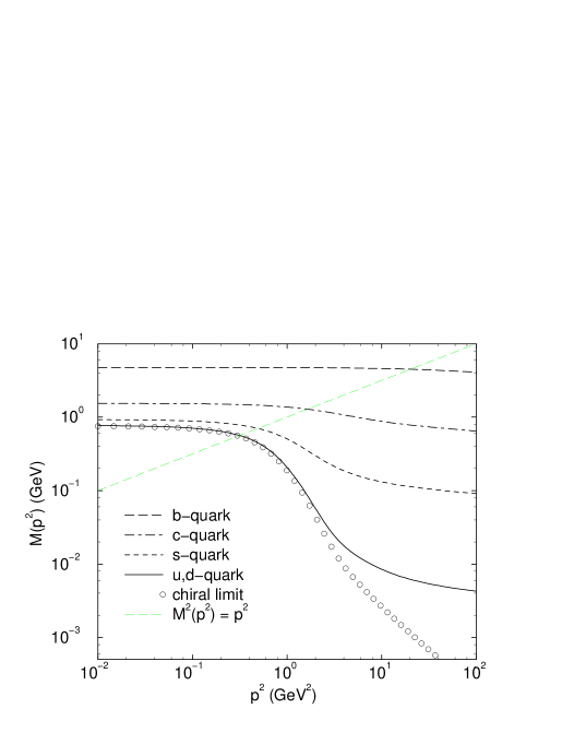
FIG. 1.: Quark mass function obtained as a solution of Eq. (2) using $D_{\mu\nu}(k)$ and $\Gamma^{fa}_{\nu}(q,p)$ from Ref. [13] and current-quark masses, fixed at $\zeta=19\,$GeV: $m_{u,d}^{\zeta}=3.7\,$MeV, $m_{s}^{\zeta}=82\,$MeV, $m_{c}^{\zeta}=0.58\,$GeV and $m_{b}^{\zeta}=3.8\,$GeV. The indicated solutions of $M^{2}(p^{2})=p^{2}$ define the Euclidean constituent-quark mass, $M^{E}_{f}$, which takes the values: $M^{E}_{u}=0.56\,$GeV, $M^{E}_{s}=0.70\,$GeV, $M^{E}_{c}=1.3\,$GeV, $M^{E}_{b}=4.6\,$GeV.

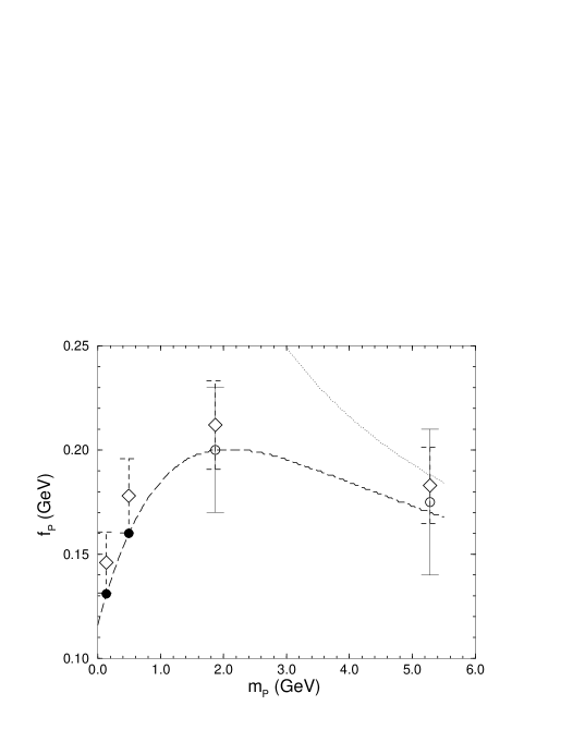
FIG. 2.: Experimental values of $f_{\pi,K}$, filled circles; lattice estimates of $f_{D,B}$ in Eq. (14), open circles; our calculated values of $f_{\pi,K,D,B}$, diamonds, see Sec. VII. (We estimate a theoretical error of 10%.) The dashed line is a fit to the experimental values and lattice estimates: $f_{P}^{2}=(0.013+0.028\,m_{P})/(1+0.055\,m_{P}+0.15\,m_{P}^{2})$, which exhibits the large-$m_{P}$ limit of Eq. (13), and the dotted line is the large-$m_{P}$ limit of this fit.

FIG. 3.: Upper panel: calculated form of the semileptonic $B\to D$ and $B\to D^{\ast}$ form factors. Lower panel: the semileptonic $B\to\pi$ and $B\to\rho$ form factors with, for comparison, data from a lattice simulation [39] and a vector dominance, monopole model: $f_{+}^{B\to\pi}(t)=0.46/(1-t/m_{B^{\ast}}^{2})$, $m_{B^{\ast}}=5.325\,$GeV, the light, short-dashed line. Monopole fits to our calculated results are given in Eqs. (115) and (116).

FIG. 4.: Calculated form of the semileptonic $D\to K$ and $D\to K^{\ast}$ (upper panel), and $D\to\pi$ and $D\to\rho$ (lower panel) form factors. Monopole fits to our calculated results are given in Eqs. (115) and (116).

FIG. 5.: Calculated form of $\xi(w)$ compared with recent experimental analyses. Our result: solid line. Experiment: short-dashed line, linear fit from Ref. [38], Eq. (118); long-dashed line, nonlinear fit from Ref. [38], Eq. (119). The two light, dotted lines are this nonlinear fit evaluated with the extreme values of $\rho^{2}$: upper line, $\rho^{2}=1.17$ and lower line, $\rho^{2}=1.89$; data points, Ref. [46].

TABLE I.: The 16 dimension-GeV quantities used in $\chi^{2}$-fitting our parameters. The weighting error is the experimental error or 10% of the experimental value, if that is greater, since we expect that to be the limit of our model’s accuracy. The values in the “Obs.” column are taken from Refs. [13, 20, 24].

	Obs.	Calc.		Obs.	Calc.
$f_{\pi}$	0.131	0.146	$m_{\pi}$	0.138	0.130
$f_{K}$	0.160	0.178	$m_{K}$	0.496	0.449
$\langle\bar{u}u\rangle^{1/3}$	0.241	0.220	$\langle\bar{s}s\rangle^{1/3}$	0.227	0.199
$\langle\bar{q}q\rangle_{\pi}^{1/3}$	0.245	0.255	$\langle\bar{q}q\rangle_{K}^{1/3}$	0.287	0.296
$f_{\rho}$	0.216	0.163	$f_{K^{\ast}}$	0.244	0.253
$\Gamma_{\rho\pi\pi}$	0.151	0.118	$\Gamma_{K^{\ast}(K\pi)}$	0.051	0.052
$f_{D}$	0.200 $\pm$ 0.030	0.213	$f_{D_{s}}$	0.251 $\pm$ 0.030	0.234
$f_{B}$	0.170 $\pm$ 0.035	0.182	$g_{BK^{\ast}\gamma}\hat{M}_{b}$	2.03 $\pm$ 0.62	2.86

TABLE II.: The 26 dimensionless quantities used in $\chi^{2}$-fitting our parameters. The weighting error is the experimental error or 10% of the experimental value, if that is greater, since we expect that to be the limit of accuracy of our model. The values in the “Obs.” column are taken from Refs. [20, 23, 37, 38, 39, 40]. The light-meson electromagnetic form factors are calculated in impulse approximation [6, 7, 8] and $\xi(w)$ is obtained from $f_{+}^{B\to D}(t)$ via Eq. (90).

	Obs.	Calc.		Obs.	Calc.
$f_{+}^{B\to D}(0)$	0.73	0.58	$f_{\pi}r_{\pi}$	0.44 $\pm$ 0.004	0.44
$F_{\pi\,(3.3\,{\rm GeV}^{2})}$	0.097 $\pm$ 0.019	0.077	B$(B\to D^{\ast})$	0.0453 $\pm$ 0.0032	0.052
$\rho^{2}$	1.53 $\pm$ 0.36	1.84	$\alpha^{B\to D^{\ast}}$	1.25 $\pm$ 0.26	0.94
$\xi(1.1)$	0.86 $\pm$ 0.03	0.84	$A_{\rm FB}^{B\to D^{\ast}}$	0.19 $\pm$ 0.031	0.24
$\xi(1.2)$	0.75 $\pm$ 0.05	0.72	B$(B\to\pi)$	(1.8 $\pm$ 0.6)${}_{\times 10^{-4}}$	2.2
$\xi(1.3)$	0.66 $\pm$ 0.06	0.63	$f^{B\to\pi}_{+\,(14.9\,{\rm GeV}^{2})}$	0.82 $\pm$ 0.17	0.82
$\xi(1.4)$	0.59 $\pm$ 0.07	0.56	$f^{B\to\pi}_{+\,(17.9\,{\rm GeV}^{2})}$	1.19 $\pm$ 0.28	1.00
$\xi(1.5)$	0.53 $\pm$ 0.08	0.50	$f^{B\to\pi}_{+\,(20.9\,{\rm GeV}^{2})}$	1.89 $\pm$ 0.53	1.28
B$(B\to D)$	0.020 $\pm$ 0.007	0.013	B$(B\to\rho)$	(2.5 $\pm$ 0.9)${}_{\times 10^{-4}}$	4.8
B$(D\to K^{\ast})$	0.047 $\pm$ 0.004	0.049	$f_{+}^{D\to K}(0)$	0.73	0.61
$\frac{V(0)}{A_{1}(0)}^{D\to K^{\ast}}$	1.89 $\pm$ 0.25	1.74	$f_{+}^{D\to\pi}(0)$	0.73	0.67
$\frac{\Gamma_{L}}{\Gamma_{T}}^{D\to K^{\ast}}$	1.23 $\pm$ 0.13	1.17	$g_{B^{\ast}B\pi}$	23.0 $\pm$ 5.0	23.2
$\frac{A_{2}(0)}{A_{1}(0)}^{D\to K^{\ast}}$	0.73 $\pm$ 0.15	0.87	$g_{D^{\ast}D\pi}$	10.0 $\pm$ 1.3	11.0

TABLE III.: Calculated values of a range of observables not included in fitting the model’s parameters, with the light-meson electromagnetic form factors calculated in impulse approximation [6, 7, 8]. The “Obs.” values are extracted from Refs. [20, 23, 24, 43].

	Obs.	Calc.		Obs.	Calc.
$f_{K}r_{K}$	0.472 $\pm$ 0.038	0.46	$-f_{K}^{2}r_{K^{0}}^{2}$	(0.19 $\pm$ 0.05)2	(0.10)2
$g_{\rho\pi\pi}$	6.05 $\pm$ 0.02	5.27	$\Gamma_{D^{\ast 0}}$ (MeV)	$<2.1$	0.020
$g_{K^{\ast}K\pi^{0}}$	6.41 $\pm$ 0.06	5.96	$\Gamma_{D^{\ast+}}$ (keV)	$<131$	37.9
$g_{\rho}$	5.03 $\pm$ 0.012	5.27	$\Gamma_{D_{s}^{\ast}D_{s}\gamma}$ (MeV)	$<1.9$	0.001
$f_{D^{\ast}}$ (GeV)		0.290	$\Gamma_{B^{\ast+}B^{+}\gamma}$ (keV)		0.030
$f_{D^{\ast}_{s}}$ (GeV)		0.298	$\Gamma_{B^{\ast 0}B^{0}\gamma}$ (keV)		0.015
$f_{B_{s}}$ (GeV)	0.195 $\pm$ 0.035	0.194	$\Gamma_{B_{s}^{\ast}B_{s}\gamma}$ (keV)		0.011
$f_{B^{\ast}}$ (GeV)		0.200	B($D^{\ast+}\!\to D^{+}\pi^{0}$)	0.306 $\pm$ 0.025	0.316
$f_{B^{\ast}_{s}}$ (GeV)		0.209	B($D^{\ast+}\!\to D^{0}\pi^{+}$)	0.683 $\pm$ 0.014	0.683
$f_{D_{s}}/f_{D}$	1.10 $\pm$ 0.06	1.10	B($D^{\ast+}\!\to D^{+}\gamma$)	0.011 ${}^{+0.021}_{-0.007}$	0.001
$f_{B_{s}}/f_{B}$	1.14 $\pm$ 0.08	1.07	B($D^{\ast 0}\!\to D^{0}\pi^{0}$)	0.619 $\pm$ 0.029	0.826
$f_{D^{\ast}}/f_{D}$		1.36	B($D^{\ast 0}\!\to D^{0}\gamma$)	0.381 $\pm$ 0.029	0.174
$f_{B^{\ast}}/f_{B}$		1.10	B($B\to K^{\ast}\gamma$)	(5.7 $\pm$ 3.3)${}_{10^{-5}}$	11.4

TABLE IV.: Calculated values of some $b\to c$ and $b\to u$ transition form factor observables not included in fitting the model’s parameters. The “Obs.” values are extracted from Refs. [20, 23].

	Obs.	Calc.		Obs.	Calc.
$A_{1}^{B\to D^{\ast}}(0)$		0.57	$A_{1}^{B\to D^{\ast}}(t_{\rm max}^{B\to D^{\ast}})$		0.88
$A_{2}^{B\to D^{\ast}}(0)$		0.56	$A_{2}^{B\to D^{\ast}}(t_{\rm max}^{B\to D^{\ast}})$		1.16
$V^{B\to D^{\ast}}(0)$		0.70	$V^{B\to D^{\ast}}(t_{\rm max}^{B\to D^{\ast}})$		1.47
$R_{1}^{B\to D^{\ast}}(1)$	1.30 $\pm$ 0.39	1.32	$R_{2}^{B\to D^{\ast}}(1)$	0.64 $\pm$ 0.29	1.04
$R_{1}^{B\to D^{\ast}}(w_{\rm max})$		1.23	$R_{2}^{B\to D^{\ast}}(w_{\rm max})$		0.98
$\alpha^{B\to\rho}$		0.60	$f_{+}^{B\to D}(t_{\rm max}^{B\to D})$		1.21
$f_{+}^{B\to\pi}(0)$		0.45	$f_{+}^{B\to\pi}(t_{\rm max}^{B\to\pi})$		3.73
$A_{1}^{B\to\rho}(0)$		0.47	$A_{1}^{B\to\rho}(t_{\rm max}^{B\to\rho})$		0.45
$A_{2}^{B\to\rho}(0)$		0.50	$A_{2}^{B\to\rho}(t_{\rm max}^{B\to\rho})$		0.81
$V^{B\to\rho}(0)$		0.68	$V^{B\to\rho}(t_{\rm max}^{B\to\rho})$		1.17
$R_{1}^{B\to\rho}(1)$		1.15	$R_{2}^{B\to\rho}(1)$		0.80
$R_{1}^{B\to\rho}(w_{\rm max})$		1.44	$R_{2}^{B\to\rho}(w_{\rm max})$		1.06

TABLE V.: Calculated values of some $c\to s$ and $c\to d$ transition form factor observables not included in fitting the model’s parameters. The “Obs.” values are extracted from Refs. [23, 20].

	Obs.	Calc.		Obs.	Calc.
B($D^{+}\to\rho^{0}$)		0.032	$\alpha^{D\to\rho}$		1.03
${\rm B}(D^{0}\to K^{-})$	0.037 $\pm$ 0.002	0.036	$\frac{{\rm B}(D\to\rho^{0})}{{\rm B}(D\to K^{\ast})}$	0.044 $\pm$ 0.034	0.065
$A_{1}^{D\to K^{\ast}}(0)$	0.56 $\pm$ 0.04	0.46	$A_{1}^{D\to K^{\ast}}(t_{\rm max}^{D\to K^{\ast}})$	0.66 $\pm$ 0.05	0.47
$A_{2}^{D\to K^{\ast}}(0)$	0.39 $\pm$ 0.08	0.40	$A_{2}^{D\to K^{\ast}}(t_{\rm max}^{D\to K^{\ast}})$	0.46 $\pm$ 0.09	0.44
$V^{D\to K^{\ast}}(0)$	1.1 $\pm$ 0.2	0.80	$V^{D\to K^{\ast}}(t_{\rm max}^{D\to K^{\ast}})$	1.4 $\pm$ 0.3	0.92
$R_{1}^{D\to K^{\ast}}(1)$		1.72	$R_{2}^{D\to K^{\ast}}(1)$		0.83
$R_{1}^{D\to K^{\ast}}(w_{\rm max})$		1.74	$R_{2}^{D\to K^{\ast}}(w_{\rm max})$		0.87
$\frac{{\rm B}(D^{0}\to\pi)}{{\rm B}(D^{0}\to K)}$	0.103 $\pm$ 0.039	0.098	$f_{+}^{D\to K}(t_{\rm max}^{D\to K})$	1.31 $\pm$ 0.04	1.11
$\frac{f_{+}^{D\to\pi}(0)}{f_{+}^{D\to K}(0)}$	1.2 $\pm$ 0.3	1.10	$f_{+}^{D\to\pi}(t_{\rm max}^{D\to\pi})$		2.18
$A_{1}^{D\to\rho}(0)$		0.60	$A_{1}^{D\to\rho}(t_{\rm max}^{D\to\rho})$		0.58
$A_{2}^{D\to\rho}(0)$		0.54	$A_{2}^{D\to\rho}(t_{\rm max}^{D\to\rho})$		0.64
$V^{D\to\rho}(0)$		1.22	$V^{D\to\rho}(t_{\rm max}^{D\to\rho})$		1.51
$R_{1}^{D\to\rho}(1)$		2.08	$R_{2}^{D\to\rho}(1)$		0.88
$R_{1}^{D\to\rho}(w_{\rm max})$		2.03	$R_{2}^{D\to\rho}(w_{\rm max})$		0.91

REFERENCES

• [1] P. C. Tandy, Prog. Part. Nucl. Phys. 39, 117 (1997).
• [2] C. D. Roberts, “Nonperturbative QCD with Modern Tools”, nucl-th/9807026.
• [3] C. D. Roberts and A. G. Williams, Prog. Part. Nucl. Phys. 33, 477 (1994).
• [4] C. D. Roberts, R. T. Cahill and J. Praschifka, Ann. Phys. 188, 20 (1988).
• [5] C. D. Roberts, R. T. Cahill, M. E. Sevior and N. Iannella, Phys. Rev. D 49, 125 (1994).
• [6] C. D. Roberts, Nucl. Phys. A 605, 475 (1996).
• [7] C. J. Burden, C. D. Roberts and M. J. Thomson, Phys. Lett. B 371, 163 (1996).
• [8] P. Maris and C. D. Roberts, Phys. Rev. C 58, 3659 (1998).
• [9] M. R. Frank, K. L. Mitchell, C. D. Roberts and P. C. Tandy, Phys. Lett. B 359, 17 (1995); R. Alkofer and C. D. Roberts, Phys. Lett. ibid 369, 101 (1996).
• [10] D. Kekez, B. Bistrovic and D. Klabucar, Int. J. Mod. Phys. A 14, 161 (1999).
• [11] M. A. Pichowsky and T.-S. H. Lee, Phys. Lett. B 379, 1 (1996); M. A. Pichowsky and T.-S. H. Lee, Phys. Rev. D 56, 1644 (1997).
• [12] F. T. Hawes and M. A. Pichowsky, Phys. Rev. C 59, 1743 (1999).
• [13] P. Maris and C. D. Roberts, Phys. Rev. C 56, 3369 (1997); P. Maris, C. D. Roberts and P. C. Tandy, Phys. Lett. B 420, 267 (1998).
• [14] D. B. Leinweber, Ann. Phys. (N.Y.) 254, 328 (1997).
• [15] P. Maris and C. D. Roberts, “Differences between Heavy and Light Quarks”, in Rostock 1997, Progress in heavy quark physics, edited by M. Beyer, T. Mannel and H. Schröder; nucl-th/9710062.
• [16] A. A. El-Hady, A. Datta, K. S. Gupta and J. P. Vary, Phys. Rev. D 55, 6780 (1997).
• [17] M. Neubert, Phys. Rep. 245, 259 (1994); M. Neubert, “Heavy quark masses, mixing angles, and spin flavor symmetry”, in The Building Blocks of Creation: From Microfermis to Megaparsecs, edited by S. Raby and T. Walker (World Scientific, Singapore 1994), hep-ph/9404296; and references therein.
• [18] M. A. Ivanov, Yu. L. Kalinovsky, P. Maris and C. D. Roberts, Phys. Rev. C 57, 1991 (1998).
• [19] V. Braun, “Light cone sum rules”, in Rostock 1997, Progress in heavy quark physics, edited by M. Beyer, T. Mannel and H. Schröder, hep-ph/9801222.
• [20] Particle Data Group (C. Caso et al.), Eur. Phys. J. C 3, 1 (1998).
• [21] P. Maris, private communication.
• [22] M. A. Ivanov, Yu. Kalinovsky, P. Maris and C. D. Roberts Phys. Lett. B 416, 29 (1998).
• [23] J. D. Richman and P. R. Burchat, Rev. Mod. Phys. 67, 893 (1995).
• [24] J. M. Flynn and C. T. Sachrajda, “Heavy Quark Physics From Lattice QCD”, hep-lat/9710057.
• [25] H. Munczek, Phys. Lett. B 175, 215 (1986); C. J. Burden, C. D. Roberts and A. G. Williams, ibid 285, 347 (1992).
• [26] A. Bender, C. D. Roberts and L. v. Smekal, Phys. Lett. B 380 (1996) 7; C. D. Roberts, in Quark Confinement and the Hadron Spectrum II, edited by N. Brambilla and G. M. Prosperi (World Scientific, Singapore, 1997), pp. 224-230.
• [27] Yu. Kalinovsky, K. L. Mitchell and C. D. Roberts, Phys. Lett. B 399, 22 (1997).
• [28] R. Alkofer, A. Bender and C. D. Roberts, Int. J. Mod. Phys. A 10, 3319 (1995).
• [29] P. Jain and H. J. Munczek, Phys. Rev. D 48, 5403 (1993).
• [30] C. J. Burden and D. S. Liu, Phys. Rev. D 55, 367 (1997).
• [31] A. Bashir, A. Kizilersu and M. R. Pennington, Phys. Rev. D 57, 1242 (1998); and references therein.
• [32] J. S. Ball and T.-W. Chiu, Phys. Rev. D 22, 2542 (1980).
• [33] D. C. Curtis and M. R. Pennington, Phys. Rev. D 46, 2663 (1992).
• [34] F. T. Hawes, C. D. Roberts and A. G. Williams, Phys. Rev. D 49, 4683 (1994).
• [35] G. Buchalla, A. J. Buraz and M. E. Lautenbacher, Rev. Mod. Phys. 68, 1125 (1996).
• [36] N. Isgur and M. B. Wise, Phys. Lett. B 232, 113 (1989); 237, 527 (1990).
• [37] S. R. Amendolia et al., Nucl. Phys. B 277, 168 (1986); C. J. Bebek, et al., Phys. Rev. D 13, 25 (1976), ibid 17, 1693 (1978);
• [38] CLEO Coll. (J. E. Duboscq et al.), Phys. Rev. Lett. 76, 3899 (1996).
• [39] UKQCD Coll. (D. R. Burford et al.), Nucl. Phys. B 447, 425 (1995).
• [40] V. M. Belyaev, V. M. Braun, A. Khodjamirian and R. Rückl, Phys. Rev. D 51, 6177 (1995).
• [41] For example, S. Capstick and B. D. Keister, “Baryon magnetic moments in a relativistic quark model”, nucl-th/9611055.
• [42] M. A. Pichowsky, private communication.
• [43] S. R. Amendolia, et al., Phys. Lett. B 178, 435 (1986); W. Molzon, et al., Phys. Rev. Lett. 41, 1213 (1978).
• [44] M. A. Ivanov, O. E. Khomutenko and T. Mitzutani, Phys. Rev. D 46, 3817 (1992); M. A. Ivanov and Yu. M. Valit, Zeit. Phys. C 67, 633 (1995); M. A. Ivanov and Yu. M. Valit, “Heavy-to-light form factors in the quark model with heavy infrapropagators”, hep-ph/9606404, Few-Body Syst. (to be published).
• [45] N. B. Demchuk, I. L. Grach, I. M. Narodetski and S. Simula, Phys. Atom. Nucl. 59, 2152 (1996).
• [46] ARGUS Collaboration, Z. Phys. C 57, 249 (1993).
Refer to caption