On local and global equilibrium in heavy ion collisions

Abstract

The thermal model is commonly used in two different ways for the description of hadron production in ultra-relativistic heavy ion collision. One is the application of the thermal model to $4\pi$ integrated data and the other is the thermal description of central d$N$/d$y$ ratios. While the first method implicitly assumes global equilibrium the other scenario assumes Bjorken scaling within the investigated rapidity range. Both assumptions are only approximations for real physical collision systems. We study the impact of both approximations for the extraction of thermal parameters on the exemplary case of S+S collisions at SPS energies. The particle distributions are modeled by a hydrodynamical description of the relevant collision system.

I Introduction

One goal of the studies of high energy collisions is the understanding of the inclusive hadron production [1]. A relevant question is whether the hadron production is dominated by phase space and statistical laws or by dynamical constraints of the underlying theory of the strong interaction. There is strong evidence that even in elementary collisions like $e^{+}e^{-}$ or pp at sufficiently high energies the dominant factor is a statistical filling of phase space [2, 3].

In heavy ion collisions one may be even closer to thermodynamic behaviour due to secondary interactions. Therefore a big effort is going on to study thermal behaviour in these collisions by microscopic models [4, 5, 6] as well as to classify directly the experimental final hadronic state by a thermal model [7, 8, 9, 10, 11, 12, 13, 14, 15, 16, 17, 18]. While within the thermal model applied at low incident energies the whole system may be regarded as one fireball in approximate global thermal and chemical equilibrium this is not anymore justified in ultra-relativistic heavy ion collisions. The incoming nucleons are only partly decelerated and the leading protons cannot equilibrate with the mesons in the center. However, the assumption of local thermal equilibrium might still be a valid assumption in these reactions.

If there is only local thermal equilibrium a fundamental problem arises in analyzing particle yields directly from experiment. A measured hadron does not tell us from which spatial region it comes from. In principle a model is needed which provides the spatial information about the particle production, like the hydrodynamic model or so called event generators. On the other side one may try to analyze chemical equilibration of particle production in ultra-relativistic heavy ion collisions directly from the measured particles without a detailed model about spatial differences in thermodynamic quantities. This is done in two different ways where both methods make necessarily some compromise.

The first method is to restrict oneself to a limited region in momentum space (e.g. around midrapidity) and to assume that the considered region in rapidity corresponds to a homogeneous spatial region in thermal equilibrium, i.e. all thermal parameters are constant over that region [7, 8, 9, 10, 11, 12, 13, 14, 15]. This procedure has the disadvantage that there is no one-to-one correspondence of spatial regions to regions in momentum (rapidity) space. One local cell contributes in general to different rapidity regions and even differently for particles of different mass. However, in the limit of infinite collision energy we have Bjorken scaling [19] which assures that along longitudinal proper time contours no spatial gradients of local variables are present. (There may still be gradients in transverse direction which we assume to be small). We recover global equilibrium again. Note that we use here and in the following the notion ”global equilibrium” if spatial regions have the same values of all intensive thermodynamic variables even if there is no causal connection between these regions. In the scaling limit a thermal and chemical analysis of particle spectra directly from experiment is possible again and in the case of RHIC and LHC this may be the only reasonable way to do it.

At SPS energies and below the rapidity spectra don’t show Bjorken scaling. Therefore a chemical analysis in a limited rapidity region might be questionable [20]. We will investigate here how well the Bjorken scaling assumption in connection with a chemical analysis works using a hydrodynamic model at SPS energies.

The mentioned problem of rapidity cuts leads to the second method for a chemical analysis, i.e. a global thermal model to $4\pi$ integrated data [16, 17, 18]. This method implicitly assumes global chemical equilibrium in the above mentioned sense. This assumption is less and less justified the smaller the colliding nuclei are and the higher the collision energy is. In S+S collisions at CERN-SPS a clear deviation from global equilibrium between pions and net protons is seen in that rapidity spectra [21]. In our study here we first like to address the question about the error of a global thermal fit to $4\pi$ integrated data in the case of only local equilibrium.

II Local and global equilibrium

Let us assume that particles decouple (freeze-out) from spatial regions which build up a continuous 3-dim freeze-out surface $\Sigma^{\mu}$ embedded in the 4-dim space-time. Along this surface we assume further to have local thermal and chemical equilibrium, but the thermal parameters may vary along this surface. The local particle densities $\rho_{i}(x)$ are then given by the local thermal parameters, temperature $T(x)$, baryon chemical potential $\mu_{\rm B}(x)$, and strangeness chemical potential $\mu_{\rm S}(x)$:

$$\rho_{i}(x)=(2J_{i}+1)\,\frac{T(x)}{2\pi^{2}}\sum_{j=1}^{\infty}(\mp 1)^{j+1}\;\exp[j(\mu_{\rm B}(x)B_{i}+\mu_{\rm S}(x)S_{i})]\;\frac{m_{i}^{2}}{j}\;{\rm K}_{2}(\frac{jm_{i}}{T(x)})\;,$$ (1)

where $J_{i}$ is the spin degeneracy, $B_{i}$ the baryon number, $S_{i}$ the strangeness, $m_{i}$ the mass of particle $i$ and the $-$ ($+$) sign is for fermions (bosons), respectively. We neglect possible suppression factors like strangeness suppression $\gamma_{\rm s}(x)$ etc which are needed if only relative chemical equilibrium is present [22]. We also assume that strangeness is conserved locally, i.e. the net strangeness density is zero everywhere. Thus $\mu_{\rm S}(x)$ can be expressed locally as a function of $T(x)$ and $\mu_{\rm B}(x)$. The multiplicity of a particle species $i$ is calculated by

$$N_{i}^{\rm local}=\int\limits_{\Sigma(x)}{\rm d}^{3}\sigma_{\mu}(x)\;j_{i}^{\mu}[T(x),\mu_{\rm B}(x),\mu_{\rm S}(x)]\;,$$ (2)

where $j_{i}^{\mu}$ is the particle current of species $i$. We use the definition of Eckart [23] for the four velocity $u^{\mu}$ and we can therefore decompose the current $j_{i}^{\mu}(x)=\rho_{i}(x)u^{\mu}(x)$ into the product of the local rest frame density $\rho_{i}(x)$ and the four velocity $u^{\mu}(x)$.

In the case of a global thermal fit one assumes that all thermal parameters are constant and thus the multiplicities are given by

$$N_{i}^{\rm global}(T,\mu_{\rm B},\mu_{\rm S})=\int\limits_{\Sigma(x)}{\rm d}^{3}\sigma_{\mu}(x)\;\rho_{i}(T,\mu_{\rm B},\mu_{\rm S})\;u^{\mu}(x)=\rho_{i}(T,\mu_{\rm B},\mu_{\rm S})\;V\;,$$ (3)

where $V=\int_{\Sigma}{\rm d}^{3}\sigma_{\mu}(x)\;u^{\mu}(x)$ is the Lorentz invariant comoving eigen volume. We define the freeze-out average of a thermal parameter $\cal O$ by

$$\langle{\cal O}\rangle=\frac{\int_{\Sigma}{\rm d}^{3}\sigma_{\mu}(x)\;u^{\mu}(x)\;{\cal O}(x)}{V}\;.$$ (4)

Next we define the global fit thermal parameters ${\cal O}^{\rm fit}$ as the parameters which give the minimum $\chi^{2}$ to experimental data or in our study case to the $N_{i}^{\rm local}$ by

$$\chi^{2}(V^{\rm fit},T^{\rm fit},\mu_{\rm B}^{\rm fit})=\sum\limits_{i}\;\frac{\left[N_{i}^{\rm global}(V^{\rm fit},T^{\rm fit},\mu_{\rm B}^{\rm fit})-N^{\rm local}_{i}\right]^{2}}{\sigma_{i}^{2}}={\rm Min}\;\chi^{2}(V,T,\mu_{\rm B})\;.$$ (5)

For small variations of the freeze-out parameters along the freeze-out surface we have the following approximate relation:

$$N^{\rm local}_{i}({\rm d}^{3}\sigma_{\mu}(x))\approx N^{\rm global}_{i}\left(T^{\rm fit},\mu_{\rm B}^{\rm fit},\mu_{\rm S}^{\rm fit}\right)\approx N^{\rm global}_{i}\Big{(}\langle T\rangle,\langle\mu_{\rm B}\rangle,\langle\mu_{\rm S}\rangle\Big{)}\;.$$ (6)

However, in general all three quantities of Eq. (6) are different. Here we like to study the validity of Eq. (6) for a realistic example in order to get a feeling about the goodness of a global fit to particle yields which arise from a system which is only in local but not in global equilibrium.

III The hydrodynamical study case of S+S collisions

The minimal deviation from global equilibrium forced by the experimental spectra is that the baryon density differs locally in space. So far there is no convincing evidence of a local change in temperature and therefore it is usually assumed to be constant (but see also [25]). A realistic freeze-out surface with constant $T$ but varying baryon density and thus varying $\mu_{B}$ and $\mu_{S}$ is naturally provided by a hydrodynamical simulation [26]. Hydrodynamics by definition assumes local thermal and chemical equilibrium.

We take as an example for our studies S+S collisions at CERN-SPS since this collision system shows the largest discrepancies in the proton and pion rapidity distribution and therefore deviations from global equilibrium. We perform a hydrodynamical simulation of S+S collisions with the same initial conditions and in the same way as described in reference [27]. The only difference is that the freeze-out hypersurface is defined now on the contour of constant temperature $T=140$ MeV. The temperature and the chemical potentials follow from the local energy density and baryon density with the help of the used equation of state which was defined in [28] and labeled as EOS A. This equation of state contains very few hadronic resonances. In order to have a typical resonance spectrum for a chemical analysis we use the resonance spectrum up to a mass of 1.7 GeV for calculating the particle spectra. This introduces a small inconsistency since the equation of state in the hydrodynamical evolution is different from the equation of state used for particle spectra. However, at the low freeze-out temperature of 140 MeV the higher resonance states are of minor importance. We show that the calculated freeze-out hypersurface is still compatible with the higher number of resonance states by comparing the resulting spectra with experiments. In Figure 1 we show as solid lines the $h^{-}$ and net proton rapidity and transverse mass distributions. The spectra are calculated as described in [28] using the description of Cooper and Frye [29]. We see that the calculated spectra are still in reasonable agreement with the data despite the use of the larger resonance input.

We now have a model system which is clearly out of global chemical equilibrium. In order to show the deviations from global equilibrium, we plot in Figure 2 the distribution of sub-volumes ${\rm d}V/{\rm d}\mu_{\rm B}$ as function of $\mu_{\rm B}$ as they result from our hydrodynamical simulation. The width in $\mu_{\rm B}$ is of order 100 MeV around the average of $\langle\mu_{\rm B}\rangle=193$ MeV. We see a large spread in $\mu_{B}$ indicating that there is a large deviation from global chemical equilibrium with respect to baryon number.

The resulting spectra are integrated over $4\pi$ and the multiplicities $N_{i}^{\rm local}$ are shown in Table I. In order to perform a $\chi^{2}$ fit we give these yields a relative error as typical for experiment [20] shown in brackets in Table I.

In a first attempt to describe the local yields one may take a global equilibrated thermal model with parameters resulting from averaging over the freeze-out hypersurface. We first take as chemical potential for the global description the averaged values $\langle\mu_{\rm B}\rangle$ and $\langle\mu_{\rm S}\rangle$. The result is given in the third column of Table I. All yields are underpredicted. Mesons come out right but baryons and anti-baryons yields are too small. The reason is that baryon yields are proportional to the baryon fugacity $\lambda_{\rm B}=\exp(\mu_{\rm B}/T)$ and $\langle\mu_{\rm B}\rangle\leq T\ln\langle\lambda_{\rm B}\rangle$. In the case of the anti-baryons we have $\exp(-\langle\mu_{\rm B}\rangle/T)\leq\langle\lambda_{\rm B}^{-1}\rangle$.

Using the average chemical potential leads in a global model to a reduction in the total baryon number. In order to avoid this problem one may use $\langle\lambda_{\rm B}\rangle$ and $\langle\lambda_{\rm S}\rangle$ as parameters in the global model. Since the baryon yields are proportional to $\lambda_{\rm B}$ in Boltzmann approximation the local and global numbers for non-strange baryons are the same up to minor corrections due to resonance decays and Fermi statistic. The result of such a calculation is shown in the fourth column of Table I. Such a scenario, however, leads to large discrepancies for the anti-baryons. Therefore such a description is not satisfactory, either.

Now we perform a fit to the local yields with a global thermal model. We take as fit parameters the volume $V$, temperature $T$, and the baryon chemical potential $\mu_{\rm B}$. $\mu_{\rm S}$ is determined by the requirement of strangeness neutrality and not used as a fit parameter. The result of the fit is shown in Table I, too. We recover in this fit nearly the input temperature and get a $\mu_{\rm B}^{\rm fit}=205.7$ MeV which is between the average $\langle\mu_{\rm B}\rangle=193.2$ and the $\mu_{\rm B}$ resulting from the average $\langle\lambda_{\rm B}\rangle$, $\mu_{\rm B}=218.4$ MeV. The deviations of individual yields of the global fit from the local integrated ones are small. The average deviation is of order 4%. The largest deviations are of order 10% for the anti-nucleons and the $\Omega$.

We conclude that the performance of a global thermal fit to $4\pi$ integrated data is fine because the deviations in temperature and volume from the exact numbers are small in the studied case of S+S collisions at SPS energies. We expect that going to larger nuclei and to smaller energies the amount of stopping increases and therefore the assumption of global equilibrium for extracting thermal parameters is even more reliable.

IV Rapidity cuts

Next we study the influence of cuts in rapidity on the extraction of thermal parameters. For all particles in Table I we integrate the corresponding spectra of the hydrodynamical simulation only over a finite interval in rapidity similar to our studies in [20]. The resulting particle yields are fitted in the same way as done before in case of $4\pi$ yields. This means that we assume Bjorken scaling in the sense that the multiplicities of particles in a finite rapidity range are still given by Eqs. (3,1). The resulting thermal parameters are shown in Table II. Before discussing the result of that exercise we construct two hypothetical cases for particle production in order to compare with. First we take the result of the hydrodynamical simulation and give every fluid cell on the freeze-out surface by hand a constant $\mu_{\rm B}=140\;{\rm MeV}\times\ln{\langle\lambda_{\rm B}\rangle}=218.4$ MeV. Then we have a system in global equilibrium, but still exhibiting the same flow in longitudinal and transverse direction as in the hydrodynamical simulation. Some of the resulting spectra are shown in Figure 1. The spectra are integrated over finite rapidity intervals and fitted with the global thermal model as done before. The resulting thermal parameters are shown in Table III. Table IV shows the result of the same procedure applied to the spectra of a static fireball with the same volume as the hydrodynamical simulation. The spectra are also shown in Figure 1.

In case of the static fireball with no flow, we see the largest influence of the cuts. The extracted temperature and $\mu_{\rm B}$ change considerably. Also the $\chi^{2}$ increases drastically going to smaller rapidity windows. We conclude that a thermal analysis in a limited rapidity interval for a static fireball is unreasonable if the analyzed rapidity interval is smaller than the thermal width of the lightest particle.

In the case of global equilibrium with longitudinal flow the picture changes. Even though we don’t see Bjorken scaling in the rapidity spectra of Figure 1 the extracted thermal parameters are rather constant and the quality of the fit stays acceptable even for the smallest rapidity window (see Table III). We see a tendency of increasing temperature and $\mu_{\rm B}$ with decreasing rapidity interval. This increase is artificially induced by the rapidity cuts but much weaker than in the case of the static fireball. Since at AGS energies and especially at SIS energies we expect less longitudinal flow, the artificial increase of the fitted temperature due to rapidity cuts around midrapidity may be larger.

In the hydrodynamic case of Table II we see a drastic decrease of $\mu_{\rm B}$ due to the baryon hole at midrapidity. The temperature, however, shows a very similar, only very small increase as in the case of global equilibrium with flow and may therefore be attributed to an artificial increase due to rapidity cuts. The quality of the fit is rather independent of the cut. In the same exercise [20] with the yields from RQMD [30] we saw a larger increase of $\chi^{2}$ with decreasing rapidity window and a larger change of thermal parameters e.g. temperature. This is due to the fact that RQMD yields are not in perfect local thermal and chemical equilibrium as it is assumed here. Especially the strange hadron production is quite different in the central region compared to the fragmentation regions. In other words, in the study of rapidity cuts within the RQMD model purely kinematic bias on thermal parameters cannot be separated from the impact of different physics in central regions compared to fragmentation regions. This is different from our study here, where any changes in the thermal parameters of tables III and IV are artificial changes due to improper kinematic cuts.

We summarize that a thermal fit to yields or ratios in a limited rapidity region gives reasonable results as long as there is large enough longitudinal flow.

V Conclusion

We have studied the impact of two approximations often used in the thermal analysis of experimental particle ratios and yields. We have done this studies for the exemplary case of S+S collisions at 200 A GeV. First we have shown that in the case of only local equilibrium a thermal description of the $4\pi$ integrated data by a global thermal model leads to deviations. The reason is that in general the average particle density $\langle\rho_{i}\rangle$ is different from the density resulting from average parameters, i.e.

$$\langle\rho_{i}[T(x),\mu_{\rm B}(x),\mu_{\rm S}(x)]\rangle\neq\rho_{i}(\langle T\rangle,\langle\mu_{\rm B}\rangle,\langle\mu_{\rm S}\rangle)\;.$$ (7)

The deviations depend on how the average is taken and can be as large as 20%.

Minimal deviations are achieved by performing a $\chi^{2}$-fit to the $4\pi$ integrated yields from a hydrodynamic simulation with local chemical equilibrium. Such fits reproduce the constant input temperature up to a few percent and lead to a $\mu_{\rm B}$ which is of the order of the average $\langle\mu_{\rm B}\rangle$. The deviations are generally small (up to 10%). The quality of a global thermal model in case of only local equilibrium in other cases than studied here, e.g. local variations of temperature, larger variations in the local baryon density, etc. have to be investigated individually. However, we think that the result of a reasonable description of yields from a only local equilibrated system by a global model will to a large extend remain valid.

We also studied the influence of rapidity cuts on the extraction of thermal model parameters. We explicitly showed that in a system without longitudinal flow the rapidity cuts lead to serious problems. In the case of S+S collisions at SPS, however, the cuts don’t spoil the extraction of the temperature but lead to smaller central $\mu_{\rm B}$ as it is expected from the dip in proton rapidity spectra. We conclude that at SPS energies already enough longitudinal flow is present to justify the Bjorken scaling assumption, in which case the fitted thermal parameters are independent of rapidity cuts.

The decision which of both methods should be used for a chemical analysis depends on the amount of longitudinal flow in the system. For low energies and large systems a $4\pi$ analysis is recommended while for small systems and high energies the analysis of d$N$/d$y$ around midrapidity should be done. We have shown that for S+S collision at SPS energies both methods give reasonable results. For RHIC and LHC an analysis in the central d$N$/d$y$ is recommended while for lower energies, especially at GSI we strongly recommend to analyze the $4\pi$ integrated data.

TABLE I.: $4\pi$ particle yields: hydrodynamical simulation of S+S collisions with local varying baryon density (second column); global thermal model using the average $\langle\mu_{\rm B}\rangle$ and $\langle\mu_{\rm S}\rangle$ (third column) or $\langle\lambda_{\rm B}\rangle$ and $\langle\lambda_{\rm S}\rangle$ (fourth column) of the hydrodynamical simulation; global thermal fit (fifth column) to the yields of the second column. The errors in brackets of column 2 are used for the $\chi^{2}$ fit and are motivated by typical experimental errors [20]. The numbers in square brackets give the percentage of deviation from mean numbers of the local yields of column 2.

particle	$N^{\rm local}$		$N^{\rm global}$		$N^{\rm global}$		$N^{\rm global}$
parameter	hydro yields		$\langle\mu_{\rm B}\rangle$,$\langle\mu_{\rm S}\rangle$		$\langle\lambda_{\rm B}\rangle$,$\langle\lambda_{\rm S}\rangle$		fit
$p$	14.95	($\pm$0.91)	12.49	[-16.4%]	14.95	[0.0%]	14.17	[-5.2%]
$\bar{p}$	0.879	($\pm$0.31)	0.796	[-9.4%]	0.665	[-24.3%]	0.786	[-10.6%]
$n$	14.90	($\pm$0.91)	12.45	[-16.4%]	14.90	[0.0%]	14.12	[-5.2%]
$\bar{n}$	0.875	($\pm$0.30)	0.793	[-9.4%]	0.663	[-24.3%]	0.783	[-10.5%]
$\pi^{+}$	81.06	($\pm$2.51)	79.83	[-1.5%]	80.96	[-0.1%]	80.96	[-0.1%]
$\pi^{-}$	81.06	($\pm$2.51)	79.79	[-1.5%]	80.91	[-0.1%]	80.91	[-0.1%]
$\pi^{0}$	90.51	($\pm$2.81)	89.13	[-1.5%]	90.28	[-0.2%]	90.39	[-0.1%]
$K^{+}$	16.62	($\pm$0.53)	16.33	[-1.7%]	16.45	[-1.0%]	16.77	[0.9%]
$K^{-}$	11.34	($\pm$0.66)	11.18	[-1.4%]	11.13	[-1.8%]	11.24	[-0.8%]
$K^{0}_{\rm s}$	13.62	($\pm$2.21)	13.39	[-1.6%]	13.43	[-1.3%]	13.64	[0.1%]
$\phi$	1.43	($\pm$0.19)	1.43	[-0.2%]	1.43	[-0.2%]	1.49	[4.2%]
$\Lambda$	5.74	($\pm$0.61)	5.20	[-9.3%]	6.18	[7.6%]	5.89	[2.6%]
$\bar{\Lambda}$	0.541	($\pm$0.099)	0.507	[-6.2%]	0.428	[-21.0%]	0.513	[-5.1%]
$\Sigma^{+}$	1.63	($\pm$0.17)	1.48	[-9.3%]	1.75	[7.6%]	1.67	[2.5%]
$\bar{\Sigma}^{+}$	0.154	($\pm$0.028)	0.144	[-6.3%]	0.121	[-21.0%]	0.146	[-5.2%]
$\Sigma^{0}$	1.61	($\pm$0.17)	1.46	[-9.3%]	1.73	[7.6%]	1.65	[2.5%]
$\bar{\Sigma}^{0}$	0.152	($\pm$0.028)	0.142	[-6.3%]	0.120	[-21.0%]	0.144	[-5.2%]
$\Sigma^{-}$	1.57	($\pm$0.17)	1.42	[-9.3%]	1.69	[7.6%]	1.61	[2.6%]
$\bar{\Sigma}^{-}$	0.148	($\pm$0.027)	0.139	[-6.3%]	0.117	[-21.0%]	0.141	[-5.1%]
$\Xi^{0}$	0.659	($\pm$0.066)	0.630	[-4.4%]	0.742	[12.5%]	0.710	[7.7%]
$\bar{\Xi}^{0}$	0.097	($\pm$0.014)	0.094	[-3.5%]	0.080	[-18.1%]	0.097	[-0.1%]
$\Xi^{-}$	0.644	($\pm$0.064)	0.615	[-4.4%]	0.725	[12.5%]	0.694	[7.8%]
$\bar{\Xi}^{-}$	0.095	($\pm$0.014)	0.092	[-3.5%]	0.078	[-18.1%]	0.095	[-0.0%]
$\Omega^{-}$	0.073	($\pm$0.017)	0.072	[-1.6%]	0.084	[14.9%]	0.082	[12.3%]
$\bar{\Omega}^{-}$	0.017	($\pm$0.006)	0.016	[-1.5%]	0.014	[-15.7%]	0.018	[6.0%]
$T$ (MeV)	$\langle 140.0\rangle$		140.0		140.0		141.8	($\pm$1.2)
$V$ (fm3)	1220		1220		1220		1134	($\pm$71)
$\!\!\mu_{\rm B}$(MeV)	$\langle 193.2\rangle$		193.2		218.4		205.7	($\pm$5.3)
$\!\!\mu_{\rm S}$(MeV)	$\langle 29.9\rangle$		29.9		31.0		31.8
$\lambda_{\rm B}$	$\langle 4.758\rangle$		3.975		4.758		4.26
$\lambda_{\rm S}$	$\langle 1.248\rangle$		1.238		1.248		1.255
$\chi^{2}$			19.89/22		15.35/22		3.97/22

TABLE II.: Thermal fit to particle yields in various rapidity intervals resulting from a hydrodynamical simulation of S+S collisions at constant freeze-out temperature of $T=140$ MeV corresponding to the solid line in Figure 1. Only the resulting thermal parameters are shown.

parameter	$y\leq$0.5	$y\leq$1.0	$y\leq$1.5	$y\leq$2.0	$4\pi$
$T$(MeV)	143.4$\pm$1.2	143.5$\pm$1.2	144.0$\pm$1.2	144.0$\pm$1.2	141.8$\pm$1.2
$V$(fm3)	316$\pm$19	594$\pm$36	793$\pm$49	932$\pm$59	1134$\pm$71
$\mu_{\rm{B}}$ (MeV)	154.8$\pm$5.0	165.0$\pm$5.1	186.2$\pm$5.2	205.3$\pm$5.3	205.7$\pm$5.3
$\chi^{2}$	3.40/22	2.45/22	2.64/22	3.85/22	3.97/22

TABLE III.: Thermal fit to particle yields in various rapidity intervals resulting from a hydrodynamical simulation of S+S collisions at constant freeze-out temperature of $T=140$ MeV and taking artificially a constant $\mu_{\rm B}=218.4$ MeV at freeze-out corresponding to the dotted line in Figure 1. Only the resulting thermal parameters are shown.

parameter	$y\leq$0.5	$y\leq$1.0	$y\leq$1.5	$y\leq$2.0	$4\pi$
$T$(MeV)	143.4$\pm$1.2	143.4$\pm$1.2	143.2$\pm$1.2	142.2$\pm$1.2	140.0$\pm$1.1
$V$(fm3)	314$\pm$20	593$\pm$37	819$\pm$51	1006$\pm$61	1224$\pm$73
$\mu_{\rm{B}}$ (MeV)	226.9$\pm$5.2	226.8$\pm$5.2	226.2$\pm$5.2	223.9$\pm$5.1	218.5$\pm$5.0
$\chi^{2}$	4.37/22	3.53/22	3.07/22	2.09/22	0.050/22

Here $\chi^{2}$ should be exactly zero. The finite value is due to the numerical uncertainty resulting from the integration of discretized momentum spectra.

TABLE IV.: Thermal fit to particle yields in various rapidity intervals resulting from a static fireball with $T=140$ MeV, $\mu_{\rm B}=218.4$ MeV and $V=1220$ fm³ corresponding to the dashed line in Figure 1. Only the resulting thermal parameters are shown.

parameter	$y\leq$0.5	$y\leq$1.0	$y\leq$1.5	$y\leq$2.0	$4\pi$
$T$(MeV)	155.1$\pm$1.5	144.7$\pm$1.2	140.8$\pm$1.1	140.0$\pm$1.1	139.8$\pm$1.1
$V$(fm3)	343$\pm$26	860$\pm$54	1154$\pm$69	1225$\pm$73	1240$\pm$74
$\mu_{\rm{B}}$ (MeV)	259.0$\pm$6.1	230.7$\pm$5.3	220.6$\pm$5.0	218.7$\pm$5.0	218.4$\pm$5.0
$\chi^{2}$	61.86/22	13.44/22	1.16/22	0.092/22	0.046/22

Here $\chi^{2}$ should be exactly zero. The finite value is due to the numerical uncertainty resulting from the integration of discretized momentum spectra.

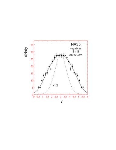
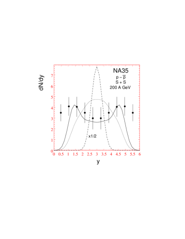
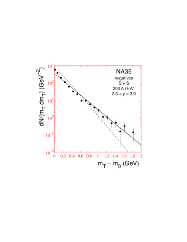
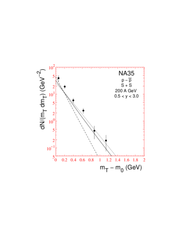
FIG. 1.: Comparison of particle spectra of a hydrodynamical simulation with freeze-out at constant temperature $T=140$ MeV (solid line) with experimental data of NA35 [24]. The dotted line results if all fluid cells at freeze-out is given by hand a constant $\mu_{\rm B}(x)=$ 218.4 MeV and corresponds therefore to a scenario of global equilibrium. The dashed line correspond to the spectra of a static fireball with the same volume as the hydrodynamical simulations as well as $T=140$ MeV and $\mu_{\rm B}=$ 218.4 MeV.

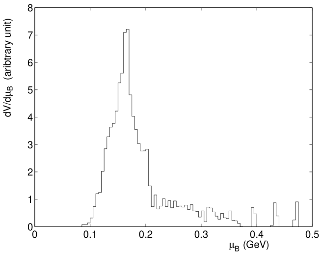
FIG. 2.: Distribution of sub-volumes $V$ having a given freeze-out baryon chemical potential $\mu_{\rm B}$.