Pairing in low-density Fermi gases
Abstract
We consider pairing in a dilute system of Fermions with a short-range interaction. While the theory is ill-defined for a contact interaction, the BCS equations can be solved in the leading order of low–energy effective field theory. The integrals are evaluated with the dimensional regularization technique, giving analytic formulas relating the pairing gap, the density, and the energy density to the two-particle scattering length.
pacs:
PACS numbers:21.30.-x, 21.65.+f,26.60.+cIn the theory of fermionic matter, the expansion about the low–density limit has been invaluable for understanding the structure of the theory and the role of the interaction. At low densities, the interaction needs only be characterized by its scattering length to get expansions for the energy density, excitation spectrum, etc.[1]. However, to our knowledge the pairing singularity has never been incorporated into this framework. We have for example only the qualitative statement in ref. [1] that the pairing singularity is logarithmic and unimportant for integrated quantities. A more quantitative statement is needed to have complete understanding of low–density fermionic matter.
Another motivation for our study is the general reexamination of nuclear physics with effective field theory which is now taking place [2, 3, 4, 5, 6, 7, 8, 9]. In the effective field theory approach, the interaction is systematically expanded in a power series in momentum with the object of getting relationships between observables such that the details of the short-distance interaction need not be parameterized. We shall show here that the BCS theory of pairing is amenable to this approach, and the low–energy theory gives finite and analytic results. Within effective field theory many results can be obtained analytically opposed to the numerical treatment of potential models. In this sense our approach complements the large body of literature of pairing in nuclear and neutron matter that is based on potential models [10, 11, 12, 13, 14, 15, 16].
We consider a Fermi gas with two-fold degeneracy interacting with a short-range attractive interaction. Examples are neutron matter or gaseous 3He. The Hamiltonian is idealized to be of the form
| (1) |
where is the kinetic energy and the volume. In effective field theory the contact interaction is the leading term in a derivative expansion of the many–body system. This limits the validity of the Hamiltonian (1) to the regime of long wave lengths or small densities. However, corrections can systematically be implemented. We have only retained terms in the contact interaction that are needed in the wave function. The BCS wave function has the form ; the energy is minimized with respect to to get the BCS equations [17]. The equation for the pairing gap is
| (2) |
where is the chemical potential. The density is given in terms of these parameters by
| (3) |
Finally, the energy density of the paired state is given by
| (4) |
Note that the last two integrals are finite, although each integrand is a sum of terms that are individually divergent.
The problem with Eq. (2) as derived is that the contact interaction is singular in three dimensions. One often introduces a cutoff to make the integrals converge. However, in effective field theory cutoffs are not explicitly introduced. Rather, the computed observables are expressed directly in terms of other physical quantities. To leading order in a low–energy expansion of the interaction, the physical quantity is the scattering length. With the same Hamiltonian, the scattering length is given by a similar divergent integral,
| (5) |
Let us now subtract equations (2) and (5) to obtain
| (6) |
Notice that the integral is now convergent and so any cutoff can be taken to infinity. Furthermore, the strength of the contact interaction , which is also an unphysical quantity, can be divided out. It is convenient to evaluate both terms of the integral (6) separately by dimensional regularization (DR) [18]. In DR, integrals of powers are zero so the second term in the integrand in (6) can be dropped. The first term can be evaluated using [19] (3.252.11),
| (7) |
where denotes the Legendre function.
We write the final result in the form
| (8) |
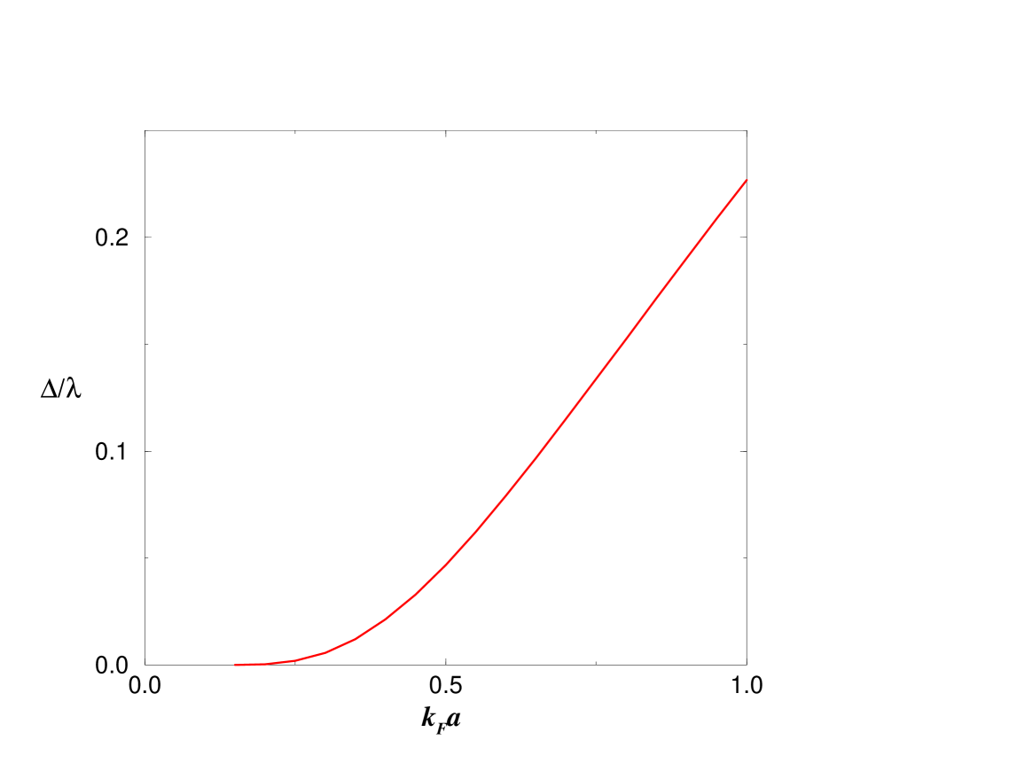
where is the Fermi momentum and . This is our main result. Eq. (8) is graphed in Fig. 1. For small values of the gap is exponentially small as in the usual BCS theory,
| (9) |
This comes about by the behavior of , which has a logarithmic singularity at [20]. Eq. (9) agrees with the result derived in ref. [14]. For large values of , the gap is proportional to , approaching .
For neutron matter the solution of eq. (8) agrees with numerical results from potential models only for small values of the Fermi momentum. The large value of the scattering length (fm) clearly limits the domain of validity of the Hamiltonian (1). In the appendix we consider pairing in the effective range approximation. This improves on the precision of the calculation in the low–density regime but does not enlarge the domain of validity.
We complete this discussion by computing the energy density (4) and the density (3). The finite integrals involved are very similar to the previous one and can be evaluated using the same DR integral, eq. (7). The density of the BCS state is given by
| (10) |
and the energy density by
| (11) |
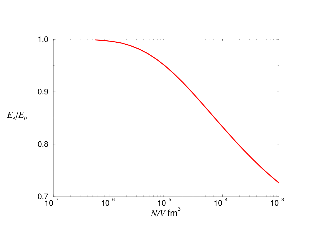
For fixed density and scattering length eqs. (8) and (10) can be solved for the pairing gap and the Fermi energy. Put into eq. (11) this yields the energy of the interacting system at fixed density. Fig. 2 shows a comparison with the energy of noninteracting neutrons. For (i.e. fm-3) pairing lowers the energy about 3% confirming the qualitative statement that the effects of pairing on the binding are mild.
Discussion — We now discuss the domain of validity of this low–density expansion. As pointed out above, the applicability of Hamiltonian (1) is limited to the regime of long wave length or small densities. The description of neutron or nuclear matter at nuclear densities requires the inclusion of the effective range and pions. Comparing with more microscopic calculations involving phenomenological potentials it appears that deviations from the low–density behavior are set by the scattering length. Similar considerations can be made for 3He where the scattering length of the Aziz potential [21] is large on an atomic scale. Many-body correlation effects will become important when . It might be possible to treat them by modifying the strength of the pairing and the density of states in eq. (1). The sign would be to increase the pairing, but we have not attempted to calculate these effects.
Another consideration is whether the low–density phase exists for fermionic systems with attractive scattering lengths. In the case of 3He, a low–density phase could only be metastable at zero temperature, because there is a finite binding of the liquid phase. However, the metastability could be quite significant, because the minimum size for a bound drop is thought to be of the order of fifty particles. Another indication of the metastability of a low–density phase is the sound velocity in the scattering length expansion. Taking the first three terms, the sound velocity is positive at all densities, and thus small deviations from uniformity are energetically unfavorable. In the case of neutron matter, it is thought that pressure is always positive as a function of density, so the low–density state would be stable.
In summary, we have considered the pairing in low–density Fermi systems within effective field theory. This model independent approach yields analytical expressions which relate the pairing gap, the density and the ground state energy to the scattering length. The analytical derivation of these results is quite interesting.
Appendix
To include the effective range we add the effective range potential
| (12) |
to the Hamiltonian (1). The gap equation then becomes
| (13) |
and is explicitly momentum dependent. We make the quadratic ansatz for the momentum dependence and obtain two coupled equations that express and in terms of (divergent) integrals. To deal with the divergencies we observe that the integrals’ dependence on the Fermi momentum is given by
| (14) |
where , and is the dimensionless function
| (15) |
In effective field theory an expansion in momenta is quite useful [3, 8]. In what follows we truncate each of the gap equations to its leading order in the Fermi momentum and obtain
| (16) | |||||
| (17) |
Obviously we have . To make contact with low energy scattering data we expand the scattering amplitude
| (18) |
up to quadratic order in momenta. The loop integral is
| (19) |
At low energies the scattering amplitude is given in terms of the scattering length and the effective range
| (20) |
Note that the divergence of the integral appearing in the gap equations (16) is similar to that of the loop integral appearing in the expression (18) for the scattering amplitude. Thus, both divergencies may be taken care off by a a renormalization of the coupling constants and . We use dimensional regularization to compute the divergent integrals. One obtains and a comparison of (18) and (20) yields and . Finally we have
| (21) |
where . This yields the final results
| (22) | |||||
| (23) |
Note that these equations add corrections of the order to the gap equation (8). These corrections are small only in the low–density regime . For a description of neutron matter (fm fm) at larger densities, at least the inclusion of pions seems to be necessary. Note also, that the gap equations (22) become singular for (i.e. ) due to the logarithmic singularity of the Legendre function for . This behavior results from the quadratic approximation for the interaction potential and the truncations in the gap equation. It is related to the change in sign of the truncated potential at [14]. Again, the introduction of pions or higher potential terms seem to be necessary to alter this behavior.
Acknowledgments
We acknowledge discussions with P. Bedaque, A. Bulgac, H. Grießhammer, D. Kaplan and M. Savage. We thank J. Hormuzdiar and S.D.H. Hsu for pointing out a correction to formula (9). This work was supported by the Dept. of Energy under Grant DE-FG-06-90ER-40561.
REFERENCES
- [1] A.A. Abrikosov, L.P. Gorkov, and I.E. Dzyaloshinski, Methods of Quantum Field Theory in Statistical Physics, (Prentice-Hall,1963).
- [2] S. Weinberg, Phys. Lett. B 251(1990)288; Nucl. Phys. B 363(1991) 3; Phys. Lett. B 295 (1992) 114
- [3] C. Ordonez, L. Ray, and U. van Kolck, Phys. Rev. Lett.72 (1994) 1982;
- [4] T.S. Park, D.P. Min and M. Rho, Phys. Rev. Lett.74 (1995) 4153; Nucl. Phys. A 596 (1996) 515
- [5] M. Luke and A.V. Manohar, Phys. Rev. D55 (1997) 4129
- [6] G.P. Lepage, nucl-th/9706029, Lectures given at 9th Jorge Andre Swieca Summer School: Particles and Fields, Sao Paulo, Brazil, 16-28 Feb 1997.
- [7] P.F. Bedaque and U. van Kolck, Phys. Lett. B 428 (1998) 221; P.F. Bedaque, H.-W. Hammer and U. van Kolck, Phys. Rev. C58 (1998) R641
- [8] D.B. Kaplan, M.J. Savage and M.B. Wise, Phys. Lett. B 424 (1998) 390; nucl-th/9802075, to appear in Nucl. Phys. B;
- [9] S.D.H. Hsu and J. Hormuzdiar, nucl-th/9811017
- [10] T.L. Ainsworth, J. Wambach, and D. Pines, Phys. Lett. B 222 (1989) 173
- [11] M. Baldo, J. Cugnon, A. Lejeune, and U. Lombardo, Nucl. Phys. A 515 (1990) 409
- [12] J.M.C. Chen, J.W. Clark, R.D. Davé, and V.V. Khodel, Nucl. Phys. A 555 (1993) 59
- [13] T. Takatsuka and R. Tamagaki, Prog. Theor. Phys. Suppl. 112 (1993) 27
- [14] V.A. Khodel, V.V. Khodel, and J.W. Clark, Nucl. Phys. A 598 (1996) 390
- [15] B.V. Carson, T. Frederico, and F.B. Guimaraes, Phys. Rev. C56 (1997) 3097
- [16] Ø. Elgarøy and M. Hjorth-Jensen, Phys. Rev. C57 (1998) 1174
- [17] J. Bardeen, L.N. Cooper, and J.R. Schrieffer, Phys. Rev. 108 (1957) 1175
- [18] J.C. Collins, Renormalization, Cambridge Univ. Press, Cambridge (1984)
- [19] I.S. Gradshteyn and I.M. Rezhik, Table of Integrals, Series and Products (1980)
- [20] A. Erdélyi (Ed.), Higher Transcendental Functions, Vol. I, McGraw Hill, N.Y. (1953)
- [21] R.A. Aziz, V.P.S. Nain, J.S. Carley, W.L. Taylor, and G.T. McConville; J. Chem. Phys.70 (1979) 4330; A.R. Janzen and R.A. Aziz, J. Chem. Phys.103 (1995) 9626