Abstract

A detailed analysis of processes of the type $NN\to d\pi$ is presented taking into account the exchange graphs of a nucleon and a pion. A large sensitivity of polarization observables to the off-mass shell effects of nucleons inside the deuteron is shown. Some of these polarization characteristics can change the sign by including these effects. The influence of the inclusion of a $P$-wave in the deuteron wave function is studied, too. The comparison of the calculation results of all the observables with the experimental data on the reaction $pp\to d\pi^{+}$ is presented.

PACS numbers: 13.60.Le,25.30Fj,25.30Rw

I Introduction

As known, pion production in $NN$ collisions, in particular the channel $NN\to d\pi$, has been investigated by many theorists and experimentalists over the last decades. An earlier study of this reaction [1, 2] and [3] show that the excitation of the $\Delta$-isobar is a crucial ingredient for explaining the observed energy dependence of the cross section. A lot of papers are based on multichannel Schrödinger equations with separable or local potentials [4, 5], [6, 7] and [8]. However, this study was performed within the nonrelativistic approach. Early attempts to develop the relativistic approach were made in [9, 10], [11, 12]. Both the pole graph, i.e. one-nucleon exchange, and the rescattering graph presented below were calculated in this paper. As shown (see, for example, [12]), this diagram can result in a dominant contribution to the cross section of the discussed process. By the calculation of this one, some approximations, in particular the factorization of nuclear matrix elements, neglect of recoil etc., were introduced which lead to an uncertainty of the final results. A more careful relativistic study of the reaction $pp\to d\pi^{+}$ was made in [13, 14, 15, 16]. The pole and rescattering graphs were shown to be insufficient to describe the experimental data; high order rescattering contributions should be taken into account. However, in this approach there was no successful description of all the polarization observables, especially the asymmetries $A_{y0}$, $iT_{11}$. Really, analyzing reactions of the type $NN\to d\pi$, there occurs a problem related to the off-mass shell effects of nucleons inside the deuteron. When the pion is absorbed by a two-nucleon pair or the deuteron, the pion energy is divided between two nucleons. So, for example, the relative momentum of the nucleon inside the deuteron increases at least by a value $\sim\sqrt{m\mu}=360MeV$ if the rest pion is absorbed by the off-shell nucleon what corresponds to intra-deuteron distances of the order of $\sim 1/\sqrt{m\mu}\simeq 0.6fm$. This means that the absorption process should be sensitive to the dynamics of the $\pi NN$ system at small distances. In this paper we concentrate mainly on the investigation of the role of these effects and the contribution of the $P$-wave of the deuteron wave function [17, 18]. The sensitivity of all the polarization observables to these effects is studied, and it is shown that some polarization characteristics can change the sign by including the off-mass shell effects of nucleons inside the deuteron. The detailed covariant formalism of the construction of the relativistic invariant amplitude of the reaction $NN\to d\pi$ and the helicity amplitudes for this process are presented in chapter 2. We analyse in detail both the pole graph, one-nucleon exchange, and the triangle diagram, i.e. the pion rescattering graph, in sections 3. The inputs by this consideration, the covariant pseudoscalar $\pi NN$ and deuteron $d\to pn$ vertices, are discussed in detail. The discussions of the obtained results and the comparison with the experimental data are presented in chapter 5. At least the conclusion is presented in the last section 6.

II General Formalism

$\bullet~{}~{}$Relativistic invariant expansion of the amplitude

We start with the basic relativistic expansion of the reaction amplitude $NN\to d\pi$ using Itzykson-Zuber conventions [19]. In the general case, the relativistic amplitude of the production of two particles of spins $1$ and $0$ by the interaction of two spin $1/2$ particles has $6$ relativistic invariant amplitudes if all particles are on-mass shell and taking $P$-invariance into account. It can be written in the following form:

$$\begin{minipage}{147.95424pt} \begin{center} \begin{picture}(6.0,4.0)\put(3.0,2.0){\circle{1.4}} \put(0.0,0.0){\makebox(6.0,4.0)[]{${\cal X}_{\mu}$}} \put(1.0,1.5){\vector(1,0){0.8}}\put(1.0,2.5){\vector(1,0){0.8}} \put(1.8,1.5){\line(1,0){0.7}}\put(1.8,2.5){\line(1,0){0.7}} \put(3.5,1.5){\line(1,0){0.15}}\put(3.8,1.5){\line(1,0){0.15}}\put(4.1,1.5){\line(1,0){0.15}}\put(4.4,1.5){\line(1,0){0.15}} \put(4.7,1.5){\vector(1,0){0.15}} \put(3.5,2.51){\line(1,0){1.265}} \put(3.55,2.45){\line(1,0){1.21}} \put(4.6,2.385){\makebox(0.2,0.1)[lb]{$>$}} \put(0.5,2.8){\parbox[b]{56.9055pt}{$\bar{v}_{\sigma_{2}}(p_{2})$}} \put(0.5,1.0){\parbox[b]{56.9055pt}{$u_{\sigma_{1}}(p_{1})$}} \put(4.5,2.8){\parbox[b]{56.9055pt}{$e^{~{}(\beta)}_{\mu}(d)$}} \put(4.8,1.05){\parbox[b]{56.9055pt}{$\varphi_{\pi}$}} \end{picture} \end{center} \end{minipage}\hfill{\cal M}_{\sigma_{2},\sigma_{1}}^{\beta}(s,t,u)=\bar{v}_{\sigma_{2}}(p_{2})\chi^{\mu}(s,t,u)u_{\sigma_{1}}(p_{1})e^{~{}(\beta)}_{\mu}(d)\varphi_{\pi}$$ (1)

where $u_{\sigma_{1}}$ and $\bar{v}_{\sigma_{2}}$ are the spinor and anti-spinor of the initial nucleons with spin projections $\sigma_{1}$ and $\sigma_{2}$, respectively; $e_{\mu}(d)$ is the deuteron polarization vector, $\varphi_{\pi}$ is the $\pi$-meson field; $s,t,u$ are the invariant variables determined in Appendix I.

For example, for the $pp\to d\pi^{+}$ process, this amplitude should be symmetrized over the initial proton states, and therefore it takes the form:

$$\bar{\cal M}_{\sigma_{2},\sigma_{1}}^{\beta}=\frac{1}{\sqrt{2}}\left[{\cal M}_{\sigma_{2},\sigma_{1}}^{\beta}(s,t,u)+{(-1)}^{\beta}{\cal M}_{\sigma_{1},\sigma_{2}}^{\beta}(s,u,t)\right]$$ (2)

The second term in (2), corresponding to the exchange of two protons, is equivalent to the exchange of the $t-$ and $u-$ variables.

The amplitude $\chi_{\mu}$ for the process $NN\to d\pi$ can be expanded over six independent amplitudes [19]:

$$\chi_{\mu}=\gamma_{5}\left({\cal X}_{1}\gamma_{\mu}+{\cal X}_{2}{p_{\mu}\over m}+{\cal X}_{3}{p^{\prime}_{\mu}\over m}+{\cal X}_{4}{p_{\mu}\over m}\widehat{p^{\prime}\over m}+{\cal X}_{5}\left(\gamma_{\mu}\widehat{p^{\prime}\over m}-\widehat{p^{\prime}\over m}\gamma_{\mu}\right)+{\cal X}_{6}{p^{\prime}_{\mu}\over m}\widehat{p^{\prime}\over m}\right).$$ (3)

$\bullet~{}~{}$Helicity formalism.

To calculate the observables, differential cross sections and polarization characteristics, it would be very helpful to construct the helicity amplitudes of the considered process $NN\to d\pi$. So, we use for this reaction the helicity formalism presented in Ref.[20]. Let us introduce initial nucleon helicities $\mu_{1},\mu_{2}$ and the final deuteron $\lambda$, and helicity amplitudes $\bar{\cal M}^{\lambda}_{\mu_{2},\mu_{1}}(W,\vartheta)$ depending on initial energy $W$ in the $N-N$ c.m.s. and scattering angle $\vartheta$ analogous to [13]. This amplitude $\bar{\cal M}^{\lambda}_{\mu_{2},\mu_{1}}(W,\vartheta)$ corresponds to the transition of the $NN$ system from the state with helicities $\mu_{1},\mu_{2}=\pm 1/2$ to the state with $\lambda=\pm 1,0$.

With respect to discrete symmetries, we have from parity conservation [20]:

$${\cal M}_{\mu_{2}\mu_{1}}^{\lambda}=\eta_{P}(-1)^{(\mu_{2}-\mu_{1})-\lambda}{\cal M}_{-\mu_{2}-\mu_{1}}^{-\lambda}=(-1)^{\mu_{2}+\mu_{1}+\lambda}{\cal M}_{-\mu_{2}-\mu_{1}}^{-\lambda}.$$ (4)

Time - reversal symmetry leads to

$${\cal M}_{\mu_{2}\mu_{1}}^{\lambda}=(-1)^{(\mu_{2}-\mu_{1})-\lambda}{\cal M}^{\mu_{2}\mu_{1}}_{\lambda},$$ (5)

where $\eta_{P}={\eta_{1}\eta_{2}\over\eta_{\pi}\eta_{d}}(-1)^{s_{d}-s_{1}-s_{2}}=(-1)$; $\eta_{i},s_{i}$ are internal parities and spins of particles.

Introducing $6$ helicity amplitudes as [13]

$$\Phi_{{}^{1}_{3}}=\bar{\cal M}_{++}^{\pm};~{}\Phi_{{}^{2}_{5}}=\bar{\cal M}_{+\pm}^{0};~{}\Phi_{{}^{4}_{6}}=\bar{\cal M}_{+-}^{\pm};$$ (6)

which satisfy the following symmetry equations

$$\Phi_{1,3}(\vartheta) = -\Phi_{1,3}(\pi-\vartheta);$$ (7)

$$\Phi_{2,5}(\vartheta) = \Phi_{2,5}(\pi-\vartheta);$$ (8)

$$\Phi_{4,6}(\vartheta) = \Phi_{6,4}(\pi-\vartheta)~{},$$ (9)

one can calculate all the observables over a range of $0<\vartheta<\pi/2$.

All the amplitudes $\bar{\cal M}_{\mu_{2}\mu_{1}}^{\lambda}(W,\vartheta)$ should vanish at forward and backward angles, and therefore we use the amplitudes introduced by Ref.[20]:

$$\bar{\cal M}_{\mu_{2}\mu_{1}}^{\lambda}(W,\vartheta)=\left(Sin{\vartheta\over 2}\right)^{|\mu+\lambda|}\left(Cos{\vartheta\over 2}\right)^{|\mu-\lambda|}\widetilde{\cal M}_{\mu_{2}\mu_{1}}^{\lambda}(W,\vartheta),$$ (10)

where $(\mu=\mu_{1}-\mu_{2})$ and $\widetilde{\cal M}_{\mu_{2}\mu_{1}}^{\lambda}(W,\vartheta)$ are the non-vanishing amplitudes at $\vartheta=0$ and $\vartheta=\pi$.

Let us present now the relation of helicity amplitudes $\{\Phi_{i}\}_{i=1}^{6}$ to the invariant functions $\{{\cal X}_{i}\}_{i=1}^{6}$. We choose the axis $z$ along the nucleon momentum $\vec{p}_{1}$. Using expansion (3), one can get the following form of the helicity amplitudes:

$$\widetilde{\Phi}_{{}^{1}_{3}} = \pm\sqrt{2}\left\{{p\over m}\left({\varepsilon\over m}{\cal X}_{2}^{a}+{\varepsilon_{d}-\varepsilon\over m}{\cal X}_{4}^{a}\right)-2{p(\varepsilon_{d}-\varepsilon)\mp k\varepsilon\over m^{2}}{\cal X}_{5}^{a}\right\}~{},$$ (11)

$$\widetilde{\Phi}_{2} = -{k\over M}\left\{{\cal X}_{1}^{s}-{\varepsilon\over m}\left({\varepsilon\over m}{\cal X}_{3}^{s}+{\varepsilon_{d}-\varepsilon\over m}{\cal X}_{6}^{s}\right)\right\}$$ (12)

$$- {p\over m}\left\{{\varepsilon_{d}\over M}\left({\varepsilon\over m}{\cal X}_{2}^{a}+{\varepsilon_{d}-\varepsilon\over m}{\cal X}_{4}^{a}\right)+2{\varepsilon\varepsilon_{d}-M^{2}\over Mm}{\cal X}_{5}^{a}\right\}Cos\vartheta~{},$$ (13)

$$\widetilde{\Phi}_{{}^{4}_{6}} = \sqrt{2}\left\{\left({p\over m}{\cal X}_{1}^{s}\mp 2{k\over m}{\cal X}_{5}^{a}\right)\mp 2{p^{2}k\over m^{3}}\left(\begin{array}[]{c}Sin^{2}\vartheta/2\\ Cos^{2}\vartheta/2\end{array}\right){\cal X}_{4}^{a}\right\}~{},$$ (16)

$$\widetilde{\Phi}_{5} = 2{p\over m}\left\{{\varepsilon_{d}\over M}\left({\cal X}_{1}^{s}+{pk\over m^{2}}{\cal X}_{4}^{a}Cos\vartheta\right)-{\varepsilon k^{2}\over Mm^{2}}{\cal X}_{6}^{s}\right\}~{}.$$ (17)

where ${\cal X}_{i}^{\{_{a}^{s}\}}(s,t,u)$ are symmetric and antisymmetric combinations ${\cal X}^{\{_{a}^{s}\}}=({\cal X}_{i}(\vartheta)\pm{\cal X}_{i}(\pi-\vartheta))/\sqrt{2}$. All symmetry properties (9) are satisfied by these amplitudes.

The helicity amplitudes are decomposed into partial waves by (see [13])

$$\bar{\cal M}_{\mu_{2}\mu_{1}}^{\lambda}(W,\vartheta)=\sum_{J}{2J+1\over 2}\left({\cal M}^{J}(W)\right)_{\mu_{2}\mu_{1}}^{\lambda}d_{\mu,-\lambda}^{J}(x)~{};$$ (18)

where $x=Cos\vartheta$, and the azimuthal angle $\varphi$ is taken to be zero. Using orthogonality relations for the $d-$function, one obtains

$$\left({\cal M}^{J}(W)\right)_{\mu_{2}\mu_{1}}^{\lambda}=\int_{-1}^{1}d_{\mu,-\lambda}^{J}(x)\bar{\cal M}_{\mu_{2}\mu_{1}}^{\lambda}(W,\vartheta)dx$$ (19)

and from symmetry relation (6) one can find that $\Phi^{J}_{{}^{4}_{6}}=(-1)^{J+1}\Phi^{J}_{{}^{6}_{4}}$.

III Reaction Mechanism

$\bullet~{}~{}$ One-nucleon exchange (ONE) and $\pi NN$-vertex.

Within the framework of the one-nucleon exchange model, the amplitude $\chi_{\mu}$ can be written in a simple form:

$$\begin{array}[]{cc}\begin{minipage}{142.26378pt} \begin{center} \begin{picture}(5.0,3.0)\put(1.0,1.0){\vector(1,0){1.1}}\put(1.0,2.2){\vector(1,0){1.1}} \put(2.1,1.0){\line(1,0){0.9}}\put(2.1,2.2){\line(1,0){0.9}} \put(3.0,1.0){\line(1,0){0.15}}\put(3.3,1.0){\line(1,0){0.15}}\put(3.6,1.0){\line(1,0){0.15}}\put(3.9,1.0){\line(1,0){0.15}}\put(4.2,1.0){\line(1,0){0.15}}\put(4.5,1.0){\line(1,0){0.15}} \put(4.8,1.0){\vector(1,0){0.2}} \put(3.0,1.0){\circle*{0.1}} \put(3.0,2.23){\line(1,0){2.0}} \put(3.0,2.17){\line(1,0){2.0}} \put(4.8,2.1){\makebox(0.2,0.1)[lb]{$>$}} \put(3.0,2.2){\circle*{0.25}} \put(3.0,1.0){\vector(0,1){0.7}} \put(3.0,1.7){\line(0,1){0.5}} \put(1.0,2.4){\parbox[b]{28.45274pt}{$p_{2}$}} \put(1.0,0.7){\parbox[b]{28.45274pt}{$p_{1}$}} \put(4.7,2.4){\parbox[b]{28.45274pt}{$d$}} \put(4.7,0.7){\parbox[b]{28.45274pt}{$\pi$}} \put(3.1,1.5){\parbox{28.45274pt}{$n$}} \put(2.8,2.5){\parbox[b]{28.45274pt}{$\bar{\Gamma}_{\mu}$}} \put(2.8,0.6){\parbox[b]{28.45274pt}{$\Gamma_{\pi}$}} \end{picture} \end{center} \end{minipage}&\chi_{\mu}=g^{+}h_{N}(n^{2})\bar{\Gamma}_{\mu}(d){\cal S}_{\cal F}(n)\Gamma_{\pi}~{},\end{array}$$ (20)

where $\bar{\Gamma}_{\mu}(d)$ is the deuteron vertex $pn\to d$ with one off-mass shell nucleon, ${\cal S}_{\cal F}(n)=\left(\widehat{n}-m+i0\right)^{-1}$ is the fermion propagator; the value of the coupling constant is $g^{+}=\sqrt{2}g^{0}=\sqrt{2}g~{},~{}~{}g^{2}/4\pi=14.7~{}$, and $n^{2}=(d-p_{2})^{2}=t$; the function $h_{N}(n^{2})$ describes the vertex $NN\pi$ where one nucleon is an off-mass shell, but the other one and the pion are on-mass shell particles [13]. The vertex $\bar{\Gamma}_{\mu}(d)$ can be related to the deuteron wave function (${\cal D}{\cal W}{\cal F}$) with the help of the following equation [21, 22]:

$$\bar{\Psi}_{\mu}={\bar{\Gamma}_{\mu}\over n^{2}-m^{2}+i0}=\varphi_{1}(t)\gamma_{\mu}+\varphi_{2}(t){n_{\mu}\over m}+\left(\varphi_{3}(t)\gamma_{\mu}+\varphi_{4}(t){n_{\mu}\over m}\right){\widehat{n}-m\over m}~{}.$$ (21)

The formfactors $\varphi_{i}(t)$ are related to two large components of the ${\cal D}{\cal W}{\cal F}$ $u$ and $w$ (corresponding to the ${}^{3}{\cal S}_{1}$ and ${}^{3}{\cal D}_{1}$ states) and to small components $v_{t}$ and $v_{s}$ (corresponding to the ${}^{3}{\cal P}_{1}$ and ${}^{1}{\cal P}_{1}$ states) as in [17].

Let us discuss now the problem connected with the form of the $\pi NN$ vertex $\Gamma_{\pi}$. In the general case, it can be expanded over four covariant quantities if all particles are an off-mass shell [23]:

$$\Gamma_{\pi}=\gamma_{5}(F_{1}+F_{2}\frac{\widehat{p}_{f}+m}{m}+F_{3}\frac{\widehat{p}_{i}-m}{m}+F_{4}\frac{\widehat{p}_{f}+m}{m}\frac{\widehat{p}_{i}-m}{m})~{};$$ (22)

here $p_{i},p_{f}$ are the four-momenta of initial and final nucleons, $\{F_{i}(t;p_{i}^{2},p_{f}^{2})\}_{i=1}^{4}$ are some functions depending on the relativistic invariant transfer $t=(p_{i}-p_{f})^{2}$ and their masses $p_{i,f}^{2}$ or the so-called pion formfactors. In our case, one nucleon $(p_{f}\equiv n)$ is the off-mass shell only, and therefore we have two terms in eq.(22) instead of four because the third and the fourth ones are vanishing, taking into account the Dirac equation for a free fermion. Then, eq.(22) can be written in the form:

$$\Gamma_{\pi}=\gamma_{5}\left(F_{1}(t)+F_{2}(t)\frac{\widehat{n}+m}{m}\right)~{}=\lambda F^{{\cal P}{\cal S}}(t)\gamma_{5}+(1-\lambda)F^{{\cal P}{\cal V}}(t)\gamma_{5}{\widehat{\pi}\over 2m}~{},$$ (23)

Note, according to the so-called equivalence theorem [24] the sum of all Born graphs for elementary processes, for example the pion photoproduction on a nucleon and the other ones, is invariant under chiral transformation. This means that starting with the Lagrangian appropriate to the pseudoscalar $({\cal P}{\cal V})$ coupling, one ends up in the Lagrangian appropriate to the pseudoscalar $({\cal P}{\cal S})$ coupling by performing a chiral transformation. This equivalence theorem is related to the processes for elementary particles. But in our case, for the reaction $NN\rightarrow d\pi$ there is a bound state, a deuteron, and therefore reducing this process to the one where only elementary particles participate, we will have the diagrams of a higher order over the coupling constant than the Born graph. So, the equivalence theorem cannot be applied to our considered processes. Therefore, the vertex $\Gamma_{\pi}$ in our case can be written in the form of eq.(23) which is actually a linear combination of pseudoscalar and pseudovector coupling with the so-called mixing parameter $\lambda$.

For the on-mass shell neutron $(n^{2}=m^{2})$ and the virtual pion, we have $\Gamma_{\pi}=\gamma_{5}$. Finally, using equations (3), (21) and (23) ($n=p^{\prime}+p$), one can find the following forms of the invariant amplitudes $\{{\cal X}_{i}\}_{i=1}^{6}$

$${\cal X}_{1} = g^{+}\left\{F_{2}\varphi_{1}-2(F_{1}+F_{2})\varphi_{3}\right\}{t-m^{2}\over 2m}~{};$$ (24)

$${\cal X}_{2} = g^{+}m\left[F_{1}(\varphi_{1}+\varphi_{2})-\left\{F_{2}(\varphi_{2}+\varphi_{3}-\varphi_{4})-2F_{1}\varphi_{4}\right\}{t-m^{2}\over 2m^{2}}\right]~{};$$ (25)

$${\cal X}_{3} = g^{+}m\left[F_{1}(2\varphi_{1}+\varphi_{2})-\left\{F_{2}(\varphi_{2}+2\varphi_{3}-\varphi_{4})-2F_{1}\varphi_{4}\right\}{t-m^{2}\over 2m^{2}}\right]~{};$$ (26)

$${\cal X}_{4} = {\cal X}_{6}~{}=~{}-g^{+}m\left\{F_{1}\varphi_{2}-F_{2}{t-m^{2}\over 2m^{2}}\varphi_{4}\right\}~{};$$ (27)

$${\cal X}_{5} = g^{+}{m\over 2}\left\{F_{1}\varphi_{1}-F_{2}{t-m^{2}\over 2m^{2}}\varphi_{3}\right\}~{}.$$ (28)

Note, the amplitudes $\{{\cal X}_{i}\}_{i=1}^{6}$ satisfy the following equations: ${\cal X}_{2}-{\cal X}_{3}+2{\cal X}_{5}=0~{};~{}~{}{\cal X}_{4}={\cal X}_{6}~{}$.

The $dNN$ vertex has been studied by Buck and Gross [17] within the framework of the Gross equation of nucleon-nucleon scattering. They used a one boson exchange (OBE) model with $\pi,\rho,\omega$ and $\sigma$ exchange. In their study, they suggest that the formfactors $F^{{\cal P}{\cal S}}$ and $F^{{\cal P}{\cal V}}$ have the same $t$ - dependence, in particular $F^{{\cal P}{\cal S}}(t)=F^{{\cal P}{\cal V}}(t)=h_{N}(t)$, and consider $\lambda=0.0;0.2;0.4;0.6;0.8$ and $1.0$. In each case, the parameters of the OBE model were adjusted to reproduce the static properties of the deuteron. They found that the total probability of the small components of the ${\cal D}{\cal W}{\cal F}$: $P_{small}=\int_{0}^{\infty}p^{2}dp\left[v_{t}^{2}(p)+v_{s}^{2}(p)\right]$, increases monotonically with growing $\lambda$ from approximately $0.03\%$ for $\lambda=0$ to approximately $1.5\%$ for $\lambda=1$.

The function $h_{N}(t)$ is the nucleon formfactor caused by the virtual nucleon and can be taken by the Breit-Wigner-type form suggested by [25] and [13].

$$h_{N}(t)={m-E_{R}\over\sqrt{t}-E_{R}+i\Gamma(t)/2}~{},~{}~{}\Gamma(t)=2\bar{\alpha}\Theta(\sqrt{t}-m-\mu)exp\left\{-{\bar{\beta}\over\sqrt{t}-m-\mu}\right\}$$ (29)

at $\bar{\alpha}=0.26~{}GeV~{};~{}~{}\bar{\beta}=0.40~{}GeV~{};~{}~{}E_{R}=1.42~{}GeV$.

Let us analyse the contributions of functions $\varphi_{1},\varphi_{2}$ determining the form of ${\cal D}{\cal W}{\cal F}$ to the invariant amplitudes ${\cal X}_{i}$. It is interesting to consider the case when the off-mass shellness of the nucleon is small, e.g. $\varphi_{3}=\varphi_{4}=0$ and $\lambda=1$. In this case, we have $5$ relativistic invariant amplitudes $\{{\cal X}_{i}\}_{i=2}^{6}$ instead of $6$.

$\bullet~{}~{}$ Second-order graphs

Let us consider now the second order graph corresponding to the rescattering of the virtual $\pi$-meson by the initial nucleon. This mechanism of the $NN\to\pi d$ process has been analysed by many authors, see, for example, [12, 13]. Our procedure of the construction of the helicity amplitudes corresponding to the triangle graph is different from the ones published by [12, 13], and so we present the proof of the forms of these amplitudes briefly.

$$\begin{minipage}{170.71652pt} \begin{center} \begin{picture}(5.0,3.0)\put(0.0,2.2){\vector(1,0){0.8}} \put(0.8,2.2){\line(1,0){0.7}} \put(1.5,2.2){\vector(1,0){1.3}} \put(2.8,2.2){\line(1,0){1.1}} \put(1.5,2.2){\line(1,-1){0.36}} \put(1.9,1.8){\vector(1,-1){0.36}} \put(2.3,1.4){\line(1,-1){0.36}} \put(2.7,1.0){\vector(1,1){0.7}} \put(3.2,1.5){\line(1,1){0.7}} \put(1.5,2.2){\circle*{0.1}} \put(3.9,2.23){\line(1,0){1.5}} \put(3.9,2.17){\line(1,0){1.5}} \put(5.2,2.1){\makebox(0.2,0.1)[lb]{$>$}} \put(3.9,2.2){\circle*{0.25}} \put(0.0,1.0){\vector(1,0){0.8}} \put(0.8,1.0){\line(1,0){1.9}} \put(2.7,1.0){\line(1,0){0.35}}\put(3.15,1.0){\line(1,0){0.35}}\put(3.6,1.0){\line(1,0){0.35}}\put(4.05,1.0){\line(1,0){0.35}}\put(4.5,1.0){\line(1,0){0.35}} \put(5.0,1.0){\vector(1,0){0.37}} \put(2.7,1.0){\circle*{0.15}} \put(0.1,2.4){\parbox[b]{28.45274pt}{$p_{2}$}} \put(0.1,0.7){\parbox[b]{28.45274pt}{$p_{1}$}} \put(5.0,2.4){\parbox[b]{28.45274pt}{$d$}} \put(5.0,0.7){\parbox[b]{28.45274pt}{$\pi$}} \put(2.6,2.4){\parbox{28.45274pt}{$\eta$}} \put(3.5,1.5){\parbox{28.45274pt}{$k$}} \put(1.7,1.5){\parbox{28.45274pt}{$q$}} \put(1.3,2.45){\parbox[b]{28.45274pt}{$\Gamma_{\pi}$}} \put(3.7,2.45){\parbox[b]{28.45274pt}{$\bar{\Gamma}_{\mu}$}} \put(2.4,0.5){\parbox[b]{28.45274pt}{$f_{\pi N}^{el}$}} \end{picture} \end{center} \end{minipage}\hfill\chi_{\mu}^{sp}={g^{+}\over(2\pi)^{3}}\int h_{\pi}(q^{2}){{\cal F}_{\mu}\left(\vec{\eta},\eta_{0}=\sqrt{\vec{\eta}^{2}+m^{2}}\right)\over q^{2}-\mu^{2}}{d^{3}\eta\over 2\eta_{0}}$$ (30)

where $h_{\pi}(q^{2})$ is the pion formfactor corresponding to the off-mass shell $\pi$-meson in the intermediate state; its form has been chosen in the monopoly one $h_{\pi}(q^{2})=(\Lambda^{2}-\mu^{2})/(\Lambda^{2}-q^{2})$ as like as in [12, 26]; here $\Lambda$ is the corresponding cut-off parameter. The general form of ${\cal F}_{\mu}$ can be written as follows:

$${\cal F}_{\mu}=\Gamma_{\pi}{\cal S}_{\cal F}^{c}(\eta){\bar{\Gamma}}_{\mu}{\cal S}_{\cal F}(k)f^{el}_{\pi N}~{},$$ (31)

where $f^{el}_{\pi N}$ is the amplitude of $\pi N$ elastic scattering; it can be presented as expansion over two off-shell invariant amplitudes $f^{el}_{\pi N}=(A+B\widehat{\pi})$ which depend on four momenta. We compute A and B from the on-shell $\pi N$ partial wave amplitudes ${\cal T}_{l\pm}^{on}(s_{\pi N})$ under the assumption

$${\cal T}_{l\pm}(s_{\pi N},t_{\pi N},u_{\pi N})\approx{\cal T}_{l\pm}^{on}(s_{\pi N})~{},$$ (32)

where ${\cal T}_{l\pm}^{on}(s_{\pi N})$ are taken from the Karlsruhe-Helsinki phase shift analysis [27]. However, in the partial wave decomposition of the invariant functions, full off-shell angular momentum projectors are used for the lowest waves in the manner discussed for the $NN\to NN\pi$ reaction in Ref.[28].

Using the covariant form of the deuteron wave function $\bar{\Psi}_{\mu}$ (21), the matrix ${\cal F}_{\mu}$ (31) can be decomposed into a suitable set of invariant functions :

$${\cal F}_{\mu}=m^{2}\sum_{i}\widehat{\cal I}_{\mu}(i)a_{i}~{};$$ (33)

the matrices $\widehat{\cal I}_{\mu}(i)$ and functions $a_{i}$ are presented in Appendix III.

We are faced with a three dimensional integro - operator over the loop momentum.

$$\widehat{\cal I}^{sp}={g^{+}\over(2\pi)^{2}}\int_{0}^{\eta_{m}}{\eta^{2}d\eta\over 2\sqrt{\eta^{2}+m^{2}}}\int_{-1}^{1}{h_{\pi}(q^{2})dCos\vartheta_{\eta}\over q^{2}-\mu^{2}}\int_{0}^{2\pi}d\varphi_{\eta}~{}.$$ (34)

The square of energy $s_{\pi N}$, the momentum transfer $u_{\pi N}$ and the square of virtual pion mass $q^{2}$ do not depend on azimuth $\varphi_{\eta}$:

$$s_{\pi N}=(p_{1}+q)^{2}=s-2\sqrt{s}\eta_{0}+m^{2}~{};$$ (35)

$$u_{\pi N}=(p_{1}-q)^{2}=t~{};$$ (36)

$$q^{2}=2\left(m^{2}-\varepsilon\eta_{0}-p\eta_{3}\right)~{}.$$ (37)

Note, at $T_{p}=0.578~{}GeV$ we have:

$$\eta_{m}^{0}={s-(m+\mu)^{2}+m^{2}\over 2\sqrt{s}};~{}\eta_{m}=\sqrt{(\eta_{m}^{0})^{2}-m^{2}}\approx 0.366~{}GeV~{}.$$ (38)

In this kinematic region, the square of the pion four-vector $q^{2}$ is space-like and the pion is moderately far from its mass shell $[0>q^{2}>-0.3~{}GeV^{2}]$ whereas an active nucleon is close to its mass shell $[0.83>k^{2}>0.63~{}GeV^{2}].$

Triple integral (34) over azimuth $\varphi_{\eta}$, polar angle $\vartheta_{\eta}$ and the magnitude of three-momentum $\eta$ must be done numerically for which we used a Gauss method. There are 6 triple integrals over a complicated complex integrand for each scattering angle.

IV Observables

Using the helicity amplitudes discussed in section 2, one can calculate all the observables: differential cross section, asymmetry, deuteron tensor polarization and so on.

It is convenient to introduce hybrid reaction parameters $({\cal H}{\cal R}{\cal P})$ for the reaction $NN\to d\pi$ as [13, 20, 29]

$$(\alpha\beta\mid LM)^{Mad}=\varepsilon_{\beta}(-1)^{M}Tr\left[\sigma_{\alpha}\sigma_{\beta}\stackrel{{\scriptstyle+}}{{{\cal M}}}^{\lambda}_{\mu_{2}\mu_{1}}T_{M}^{L}(s_{d}){\cal M}^{\lambda}_{\mu_{2}\mu_{1}}\right]\Sigma^{-1}~{}.$$ (39)

with $\varepsilon_{0}=\varepsilon_{x}=1;~{}\varepsilon_{y}=\varepsilon_{z}=1$, $\sigma_{\alpha}$ and $\sigma_{\beta}$ $(\alpha,\beta=0,x,y,z)$ the Pauli spin operators for initial nucleons and $T_{M}^{L}(s_{d})$ the spin-one tensor of rank $L\leq 2$. The normalization of the ${\cal H}{\cal R}{\cal P}$ is such that $(00\mid 00)=1$. Then, the differential cross section is related to $\Sigma$ as

$$\Sigma=2\sum_{1}^{6}{\mid\Phi_{i}\mid}^{2}=4\frac{p}{k}{(\frac{m}{4\pi\sqrt{s}})}^{-2}\frac{d\sigma}{d\Omega}={1\over\sigma_{0}}\frac{d\sigma}{d\Omega}~{},$$ (40)

where $p$ and $k$ are the momenta of initial proton and final deuteron in the c.m.s. There are $4\times 4\times 9=144$ ${\cal H}{\cal R}{\cal P}$. However, since parity invariance reduces the number of independent amplitudes to six, there are only $36$ linearly independent bilinear observables. They have the following symmetry properties and relations:

$$(\alpha\beta\mid LM)~{}~{}is~{}~{}\left\{\begin{array}[]{c}real\\ imag.\end{array}\right\}~{}~{}~{}~{}if~{}~{}n_{0}+n_{y}+L~{}~{}is~{}~{}\left\{\begin{array}[]{c}even\\ odd\end{array}\right\}~{},$$ (45)

$$n_{0,y}~{}~{}is~{}~{}number~{}~{}of~{}~{}\sigma_{0,y}~{};~{}~{}$$ (46)

$$(\alpha\beta\mid LM)_{\vartheta}=(-1)^{M}(\beta\alpha\mid LM)_{\pi-\vartheta}~{};$$ (47)

$$(\alpha\beta\mid LM)=\zeta_{\alpha}\zeta_{\beta}(-1)^{L+M}(\alpha\beta\mid L-M)~{},$$ (48)

$$\zeta_{0}=\zeta_{y}=1~{};~{}~{}\zeta_{x}=\zeta_{z}=-1~{}.$$ (49)

Let us present now the expressions for the following observables in the c.m.s. using $\Phi_{i}$:

$$A_{y0} = 4Im(\Phi_{1}\Phi^{*}_{4}+\Phi_{2}\Phi^{*}_{5}+\Phi_{3}\Phi^{*}_{6})\Sigma^{-1},~{}~{}~{}A_{0y}(\theta)=A_{y0}(\pi-\theta),$$ (50)

$$A_{xz} = -4Re(\Phi_{1}\Phi^{*}_{4}+\Phi_{2}\Phi^{*}_{5}+\Phi_{3}\Phi^{*}_{6})\Sigma^{-1},~{}~{}~{}A_{zx}(\theta)=A_{xz}(\pi-\theta),$$ (51)

$$A_{zz} = -1+4(|\Phi_{4}|^{2}+|\Phi_{5}|^{2}+|\Phi_{6}|^{2})\Sigma^{-1},$$ (52)

$$A_{yy} = -1+2(|\Phi_{1}+\Phi_{3}|^{2}+|\Phi_{4}+\Phi_{6}|^{2})\Sigma^{-1},$$ (53)

$$A_{xx} = A_{zz}+2(|\Phi_{1}+\Phi_{3}|^{2}-|\Phi_{4}+\Phi_{6}|^{2})\Sigma^{-1}.$$ (54)

The expressions for the deuteron tensor polarization components are the following:

$$iT_{11} = -\sqrt{6}Im\left[(\Phi^{*}_{1}-\Phi^{*}_{3})\Phi_{2}+(\Phi^{*}_{4}-\Phi^{*}_{6})\Phi_{5}\right]\Sigma^{-1},$$ (55)

$$T_{20} = \left[1-6(|\Phi_{2}|^{2}+|\Phi_{5}|^{2})\Sigma^{-1}\right]/\sqrt{2},$$ (56)

$$T_{21} = \sqrt{6}Re\left[(\Phi^{*}_{1}-\Phi^{*}_{3})\Phi_{2}+(\Phi^{*}_{4}-\Phi^{*}_{6})\Phi_{5}\right]\Sigma^{-1},$$ (57)

$$T_{22} = 2\sqrt{3}Re(\Phi^{*}_{1}\Phi_{3}+\Phi^{*}_{4}\Phi_{6})\Sigma^{-1}=(1+3A_{yy}-\sqrt{2}T_{20})/(2\sqrt{3})~{}.$$ (58)

V Results and Discussions

In order to investigate the effect of small components of the ${\cal D}{\cal W}{\cal F}$, we have calculated the differential cross section $d\sigma/d\Omega$, polarization characteristics $A_{ii},A_{y0}$, etc. for $pp\to d\pi^{+}$ as a function of scattering angle at proton kinetic energy $T_{p}=578MeV$ corresponding to pion kinetic one $T_{\pi}=147MeV$ because at this energy the probability of $\Delta$-isobar production by the two - step mechanism is rather sizeable. All the calculated quantities are in the Madison convention and compared with the experimental data [14, 30] and partial-wave analysis (${\cal P}{\cal W}{\cal A}$) by R. A. Arndt et al. [31] (dotted curve). The cut-off parameter $\Lambda$ and the mixing one $\lambda$ corresponding to the $\pi NN$ vertex are chosen by the best fitting of the experimental cross section $d\sigma/d\Omega$ data. We have checked that the polarization curves change very little if we vary the cut-off parameter $\Lambda$.

Note that the contribution of the triangle graph is very large at intermediate initial kinetic energies and much smaller at lower energies. It is caused by a large value of the cross section of elastic $\pi N$ scattering because of a possible creation of the $\Delta$-isobar at this energy. One can stress that the application of Locher’s form ${\cal D}{\cal W}{\cal F}$ [15] does not allow one to reproduce the absolute value of the differential cross section (see Fig.(1)) over the whole region of scattering angle $\vartheta$. But using the Gross approach for the ${\cal D}{\cal W}{\cal F}$, one can describe $d\sigma/d\Omega$ at $\lambda=0.6-0.8$ rather well.

The next interesting result which can be seen from Fig.(1) is a large sensitivity of all the polarization characteristics to the small components of the ${\cal D}{\cal W}{\cal F}$. The asymmetry $A_{y0}$ and the vector polarization $iT_{11}$ calculated within the framework of Gross’s approach particularly show this large sensitivity. These quantities are interference dominated and sensitive to the phases. The results for $iT_{11}$ have a wrong sign with Locher’s form ${\cal D}{\cal W}{\cal F}$ [14]. On closer inspection, we observe that the first term in eq.(58), $(\Phi^{*}_{1}-\Phi^{*}_{3})\Phi_{2}$, is very big due to constructive interference $\Phi_{1}\approx-\Phi_{3}$. It is caused by the $N\triangle$ configuration in a relative ${\cal S}$ wave having $pp$ spin zero (${}^{1}{\cal D}_{2}$ state). The ${}^{1}{\cal D}_{2}$ partial-wave dominates making $\Phi_{1,2,3}$ large, but the results are the same contribution to $\Phi^{{\cal J}=2}_{1}$ and $\Phi^{{\cal J}=2}_{3}$ (with opposite signs caused by the relevant Wigner d-function signature). Since the contribution of $\Phi_{4,5,6}$ is negligible, the sign problem for $iT_{11}$ is therefore very sensitive to the $\Phi^{{\cal J}=0}_{2}$ (or ${}^{1}{\cal S}_{0}$) partial wave. As $iT_{11}$ is very nearly proportional to $\Phi_{2}$, the phase of $\Phi_{2}$ determines the sign of $iT_{11}$.

The right structure of the observables starts to appear gradually in the theoretical curves as one increases the mixing parameter $\lambda$ in the Buck-Gross model, that is to say, as one increases the probability of the small components in the ${\cal D}{\cal W}{\cal F}$. We have checked that this structure originates indeed from the small components $v_{t}$ and $v_{s}$ in eq.(21). If we make $v_{t}=v_{s}=0$ in the Buck-Gross model, then all curves become very similar to Locher’s ones. Similarly, if we vary the $\pi NN$ vertex given by eq.(23) by considering $\lambda$ between $0$ and $1$ but keep Locher’s ${\cal D}{\cal W}{\cal F}$, then the curves change very little again.

The proton spin correlations $A_{ii}$ are presented in Fig.(2). Actually, the data on $A_{zz}$ is the measure of the $\Phi_{4,5,6}$ magnitudes because the deviation of $A_{zz}$ from $-1$ is determined by these amplitudes (54). According to the partial-wave decomposition, $\Phi_{4}$ and $\Phi_{6}$ are the amplitudes containing only triplet spin states in the $pp$ channel. One can conclude that the magnitudes of the spin-triplet amplitudes are somewhat small. As for $A_{yy}$ and $A_{xx}$, the terms proportional to $\Phi_{1}+\Phi_{3}$ can be neglected because there is a phase relation $\Phi_{1}\approx-\Phi_{3}$. Therefore, the deviation of $A_{yy}$ and $A_{xx}$ from $-1$ is determined by $\Phi_{4,6}$ again, whereas $\Phi_{5}$ does not contribute to the numerator of $A_{yy}$.

One can also see a large sensitivity of the observables $A_{ii}$ to the used form of ${\cal D}{\cal W}{\cal F}$. The application of Gross’s approach by the construction of ${\cal D}{\cal W}{\cal F}$ [17] results in the shapes of these characteristics which are different from the corresponding ones obtained within the framework of Locher’s approach [16].

Note, the energy dependence of all the observables within the framework of the suggested approach is the subject of our next investigation.

VI Summary and Outlook

A relativistic model for the reaction $NN\to d\pi$ has been discussed in detail using two forms of the ${\cal D}{\cal W}{\cal F}$ [14] and [17]. One of them [14] was already used in the analysis of the $pp\to d\pi$ process [13] also taking into account the two-step mechanism with a virtual pion in the intermediate state. The difference between our approach and the model considered in [13] is the following. We have analysed the sensitivity of all the observables to the form of $\pi NN-$current and the choice of the ${\cal D}{\cal W}{\cal F}$ relativistic form. First of all, from the results presented in Fig.(1,2), one can see very large sensitivity of all the observables, especially of the polarization characteristics to the choice of the ${\cal D}{\cal W}{\cal F}$ form. The inclusion of the $P$-wave contribution in the ${\cal D}{\cal W}{\cal F}$ within the framework of Gross’s approach [17] results in a better description of the experimental data on the differential cross section and the polarization observables. The next interesting result is related to the extraction of some new information on the off-shell effects due to a virtual (off-shell) nucleon. Comparing the observable with the experimental data (see Fig.(1,2)), one can test the assumption, suggested by [18], of a possible form of the pion formfactor and conclude that one cannot use the mixing parameter $\lambda=1$ as like as in [14].

One can stress that the one-nucleon exchange and the pion rescattering graphs have been studied only in this paper in order to investigate very important effects: off-mass shellness of nucleon and pion, and $P-$wave contribution to the ${\cal D}{\cal W}{\cal F}$. The interactions in the initial $NN$ and final $d\pi$ states can be in principle contributed to the total amplitude of the considered reaction. However, it will be as a separate stage of this study because a more careful inclusion of elastic $NN$ and $d\pi$ interactions at intermediate energies is needed.

Finally, let us stress that there is in principle an alternative approach to study the ${\cal D}{\cal W}{\cal F}$ at small distances based on the non - nucleon or quark degree of freedom [32, 33, 34]. However, the main goal of our paper is to show the role of the conventional nucleon degrees of freedom in the deuteron by analising the processes of the type $NN\to d\pi$. Therefore, we didn’t analyse the application of quark approaches to this reaction.

Acknowledgements.

We gratefully acknowledge very helpful discussions with V. R. Pandharipande, R. Machleidt, S. Moszkovsky and E. A. Strokovsky.

VII Appendix I

$\bullet~{}~{}$ Kinematics of $NN\to d\pi$.

The ${\cal S}$-matrix element of the reaction ${\cal S}_{\sigma_{2}\sigma_{1}}^{\beta}=<\pi d,out|p_{1}p_{2},in>$ is related to the corresponding ${\cal M}$-matrix element by the following equation:

$${\cal S}_{\sigma_{2}\sigma_{1}}^{\beta}={1\over(2\pi)^{2}}{m\over{\sqrt{\varepsilon_{1}\varepsilon_{2}2\varepsilon_{\pi}2\varepsilon_{d}}}}\delta^{4}\left(\pi+d-p_{1}-p_{2}\right){\cal M}_{\sigma_{2}\sigma_{1}}^{\beta},$$ (59)

where $\beta,\sigma_{1}$ and $\sigma_{2}$ are the spin indices of deuteron polarization and spin projections of initial nucleons.

As is well-known, Mandelstam’s variables

$$s=(p_{1}+p_{2})^{2}~{}~{};~{}~{}t=(d-p_{2})^{2}~{}~{};~{}~{}u=(d-p_{1})^{2}~{}~{},$$ (60)

are related by the condition: $s+t+u=M^{2}+2m^{2}+\mu^{2}=h$.

Let us introduce the following variables:

$$P=p_{1}+p_{2}~{}~{}~{}~{}~{},~{}~{}~{}~{}~{}P^{2}=s~{}~{}~{}~{}~{};$$ (61)

$$p=(p_{1}-p_{2})/2~{}~{},~{}~{}~{}p^{\prime}=(d-\pi)/2.$$ (62)

Note,

$$p^{2}=m^{2}-{s\over 4}\leq 0~{};~{}~{}p^{\prime 2}={1\over 2}(M^{2}+\mu^{2})-{s\over 4}\leq 0~{};~{}~{}p^{\prime 2}+p^{2}={t+u\over 2}~{};$$ (63)

$$(pP)=0~{};~{}~{}(p^{\prime}P)={1\over 2}(M^{2}-\mu^{2})~{};~{}~{}(p^{\prime}p)\equiv\nu={t-u\over 4}\leq 0~{}~{}.~{}~{}~{}~{}$$ (64)

Let us now introduce two space-time four-vectors orthogonal to $P$ and $p$ :

$$N_{\mu}={1\over\sqrt{-p^{2}P^{2}}}\varepsilon_{\mu\nu\rho\sigma}p^{\prime\nu}p^{\rho}P^{\sigma}~{};~{}~{}(Np^{\prime})=0;~{}~{}~{}~{}~{}~{}~{}~{}~{}~{}$$ (65)

$$L_{\mu}={1\over\sqrt{-p^{2}P^{2}}}\varepsilon_{\mu\nu\rho\sigma}N^{\nu}p^{\rho}P^{\sigma}=\left(p^{\prime}_{\mu}-{\nu\over p^{2}}p_{\mu}\right)-{(p^{\prime}P)\over P^{2}}P_{\mu}~{};$$ (66)

$$N^{2}=L^{2}=\left\{\left(p^{\prime 2}-{\nu^{2}\over p^{2}}\right)-{(p^{\prime}P)^{2}\over P^{2}}\right\}\leq 0~{};~{}~{}(LN)=0.~{}~{}~{}$$ (67)

Then, one can get the whole system of orthogonal unit four-vectors $\{e_{\mu}^{(\sigma)}\}_{\sigma=0}^{3}$, three of them are space-like :

$$e_{\mu}^{(1)}\equiv l_{\mu}={L_{\mu}\over\sqrt{-L^{2}}}~{};~{}~{}e_{\mu}^{(2)}\equiv n_{\mu}={N_{\mu}\over\sqrt{-N^{2}}}~{};~{}~{}e_{\mu}^{(3)}\equiv e_{\mu}={p_{\mu}\over\sqrt{-p^{2}}}~{};~{}~{}$$ (68)

and one of them is time-like:

$$e_{\mu}^{(0)}={P_{\mu}\over\sqrt{P^{2}}}~{}.$$ (69)

They satisfy the following conditions :

$$g^{\mu\nu}e_{\mu}^{~{}(\sigma)}e_{\nu}^{~{}(\rho)}=g^{\sigma\rho}~{};~{}~{}~{}~{}~{}e_{\mu}^{~{}(\sigma)}e_{\nu}^{~{}(\rho)}g_{\sigma\rho}=g_{\mu\nu}~{},~{}~{}~{}~{}~{}$$ (70)

Therefore, any four-vector $a_{\mu}$ can be expanded over this unit orthogonal system, i.e.:

$$a_{\mu}=\left(ae^{(\sigma)}\right)e_{\mu}^{~{}(\rho)}g_{\sigma\rho}~{};~{}~{}a^{2}=(ae)^{2}.$$ (71)

For example, we can expand the matrix four-vector $\chi_{\mu}$ (1) over these basic vectors:

$$\chi_{\mu}=\chi_{i}e_{\mu}^{(i)}=\chi_{1}l_{\mu}+\chi_{2}n_{\mu}+\chi_{3}e_{\mu}~{},~{}~{}\chi_{i}=-\chi^{\mu}e_{\mu}^{(i)}~{}=\gamma_{5}\left(a_{i}+b_{i}{\widehat{l}}\right);~{}$$ (72)

VIII Appendix II

$\bullet~{}~{}$ Pauli’s representation of $NN\to d\pi$.

In the c.m.s., we can use the next Pauli form of the reaction amplitude

$${\cal M}_{\sigma_{2}\sigma_{1}}^{\beta}(t,u)=w^{+}_{-\sigma_{2}}\left(\vec{\chi}\vec{e}^{~{}(\beta)}\right)w_{\sigma_{1}}.$$ (73)

The vector of the reaction is parametrized in the following form:

$$\vec{\chi}=\sum_{i=1}^{6}\chi_{i}(\vec{p}^{~{}2},\vec{n}\vec{p})\cdot\vec{i}=\chi_{1}\vec{e}_{p}+\chi_{2}\vec{n}+i\chi_{3}\left[\vec{\sigma}\times\vec{e}_{p}\right]~{}$$ (74)

$$+i\chi_{4}\left[\vec{\sigma}\times\vec{n}\right]+i\chi_{5}\left(\vec{\sigma}\vec{n}\right)\left[\vec{n}\times\vec{e}_{p}\right]+i\chi_{6}\left(\vec{\sigma}\vec{e}_{p}\right)\left[\vec{n}\times\vec{e}_{p}\right];$$ (75)

where: $\vec{e}_{p}=\widehat{\vec{p}},~{}~{}\vec{n}=-\vec{e}_{d}~{};~{}~{}\vec{e}_{p}^{~{}2}=\vec{n}^{~{}2}=1~{};~{}~{}z=(\vec{n}\vec{e}_{p})~{}.$

And, finally, we have the following connection with invariant expansion (3):

$$\chi_{1} = -{p\over m}\left({\varepsilon\over m}{\cal X}_{2}+{\varepsilon_{d}-\varepsilon\over m}\left({\cal X}_{4}-2{\cal X}_{5}\right)\right);$$ (76)

$$\chi_{2} = -{k\over M}\left({\cal X}_{1}-{\varepsilon\over m}\left({\varepsilon\over m}{\cal X}_{3}+{\varepsilon_{d}-\varepsilon\over m}{\cal X}_{6}\right)\right)$$ (77)

$$- {p\over m}{\varepsilon_{d}-M\over M}\left({\varepsilon\over m}{\cal X}_{2}+{\varepsilon_{d}-\varepsilon\over m}({\cal X}_{4}-2{\cal X}_{5})+2{\varepsilon_{d}+M\over m}{\cal X}_{5}\right)z;$$ (78)

$$\chi_{3} = {p\over m}\left({\varepsilon_{d}\over M}\left({\cal X}_{1}+{pk\over m^{2}}z{\cal X}_{4}\right)-{\varepsilon k^{2}\over Mm^{2}}{\cal X}_{6}\right);$$ (79)

$$\chi_{4} = -{p\over m}\left({\varepsilon_{d}-M\over M}\left({\cal X}_{1}+{pk\over m^{2}}z{\cal X}_{4}\right)-{\varepsilon k^{2}\over Mm^{2}}{\cal X}_{6}\right)z$$ (80)

$$- {k\over m}\left({\varepsilon^{2}\over m^{2}}{\cal X}_{4}-\left({\cal X}_{4}-2{\cal X}_{5}\right)\right);$$ (81)

$$\chi_{5} = -{p\over m}\left({\varepsilon_{d}-M\over M}\left({\cal X}_{1}+{pk\over m^{2}}z{\cal X}_{4}\right)-{\varepsilon k^{2}\over Mm^{2}}{\cal X}_{6}\right);$$ (82)

$$\chi_{6} = -{k\over m}{\varepsilon-m\over m}\left({\varepsilon\over m}{\cal X}_{4}+\left({\cal X}_{4}-2{\cal X}_{5}\right)\right).$$ (83)

Helicity amplitudes (4) can be related to the corresponding Pauli amplitudes $\{\chi_{i}\}_{i=1}^{6}$ (75):

$$\widetilde{\Phi}_{{}^{1}_{3}} = \sqrt{2}\left(\mp\chi_{1}^{a}-\chi_{4}^{a}+\chi_{5}^{s}Cos\vartheta+\chi_{6}^{a}\right)~{};$$ (84)

$$\widetilde{\Phi}_{2} = \chi_{1}^{a}Cos\vartheta+\chi_{2}^{s}~{};$$ (85)

$$\widetilde{\Phi}_{{}^{4}_{6}} = \left\{\left(\chi_{3}^{s}\pm\chi_{4}^{a}\right)+2\chi_{5}^{s}\left(\begin{array}[]{c}Sin^{2}\vartheta/2\\ Cos^{2}\vartheta/2\end{array}\right)\right\}~{};$$ (88)

$$\widetilde{\Phi}_{5} = 2\chi_{3}^{s}Sin\vartheta~{}.$$ (89)

IX Appendix III

In this appendix we give explicit expressions for helicity amplitudes (4) for the rescattering diagram. The evolution of the expression for $\chi_{\mu}^{sp}$ (30) is straightforward. The spin structure operator ${\cal F}_{\mu}$ (31) here

$${1\over m^{2}}{\cal F}_{\mu}=\sum_{i=1}^{16}a_{i}\widehat{\cal I}_{\mu}(i)=\Gamma_{\pi}{(-\widehat{\eta}+m)\over m}\bar{\Psi}_{\mu}{(\widehat{k}+m)\over m}(A+B\widehat{\pi})$$ (90)

is a $4\times 4$ matrix in the spinor space and carries the label of deuteron polarization. The first six of the operators $\widehat{\cal I}_{\mu}(i)$ do not depend on the integration variable:

$$\widehat{\cal I}_{\mu}(1)=\gamma_{5}\gamma_{\mu}~{};~{}~{}\widehat{\cal I}_{\mu}(2)=\gamma_{5}{p_{\mu}\over m}~{};~{}~{}\widehat{\cal I}_{\mu}(3)=\gamma_{5}{p^{\prime}_{\mu}\over m}~{};~{}~{}$$ (91)

$$\widehat{\cal I}_{\mu}(4)=\gamma_{5}\widehat{\pi}{p_{\mu}\over m}~{};~{}~{}\widehat{\cal I}_{\mu}(5)=\gamma_{5}\widehat{\pi}{p^{\prime}_{\mu}\over m}~{};~{}~{}\widehat{\cal I}_{\mu}(6)=\gamma_{5}\gamma_{\mu}\widehat{\pi}~{}.$$ (92)

The next three of $\widehat{\cal I}_{\mu}(i)$ depend only on $\eta:$

$$\widehat{\cal I}_{\mu}(7)=\gamma_{5}{\eta_{\mu}\over m}~{};~{}~{}\widehat{\cal I}_{\mu}(8)=\gamma_{5}{\widehat{\eta}\eta_{\mu}\over m^{2}}~{};~{}~{}\widehat{\cal I}_{\mu}(9)=\gamma_{5}\left(\gamma_{\mu}{\widehat{\eta}\over m}-{\widehat{\eta}\over m}\gamma_{\mu}\right)~{}.$$ (93)

The remaining $\widehat{\cal I}_{\mu}(i)$ are:

$$\widehat{\cal I}_{\mu}(10)=\gamma_{5}{\widehat{\eta}p_{\mu}\over m^{2}}~{};~{}~{}\widehat{\cal I}_{\mu}(11)=\gamma_{5}{\widehat{\eta}p^{\prime}_{\mu}\over m}~{};~{}~{}\widehat{\cal I}_{\mu}(12)=\gamma_{5}{\eta_{\mu}\over m}\widehat{\pi}~{};~{}~{}~{}~{}~{}~{}~{}$$ (94)

$$\widehat{\cal I}_{\mu}(13)=\gamma_{5}{\widehat{\eta}p_{\mu}\over m^{2}}\widehat{\pi}~{};~{}~{}\widehat{\cal I}_{\mu}(14)=\gamma_{5}{\widehat{\eta}p^{\prime}_{\mu}\over m^{2}}\widehat{\pi}~{};~{}~{}\widehat{\cal I}_{\mu}(15)=\gamma_{5}{\widehat{\eta}\eta_{\mu}\over m^{2}}\widehat{\pi}~{}:~{}~{}$$ (95)

$$\widehat{\cal I}_{\mu}(16)=\gamma_{5}\gamma_{\mu}{\widehat{\eta}\over m}\widehat{\pi}~{}.~{}~{}~{}~{}~{}~{}~{}~{}~{}~{}~{}~{}~{}~{}~{}~{}~{}~{}~{}~{}~{}~{}~{}~{}~{}~{}~{}~{}~{}~{}$$ (96)

With little algebra, one finds

$$a_{1} = A\left(2-{q^{2}\over m^{2}}\right)\varphi_{1}+B{m^{2}-t\over m}\varphi_{1}+A{k^{2}-m^{2}\over m^{2}}\varphi_{3}~{};$$ (97)

$$a_{2} = -2A\varphi_{1}~{}=~{}a_{3}~{};~{}~{}a_{4}~{}=~{}-2B\varphi_{1}~{}=~{}a_{5}~{};$$ (98)

$$a_{6} = -{1\over m}A\varphi_{1}-B{q^{2}\over m^{2}}\varphi_{1}+B{k^{2}-m^{2}\over m^{2}}\varphi_{3}~{};$$ (99)

$$a_{7} = -2A(2\varphi_{1}+\varphi_{2})-A{q^{2}\over m^{2}}\varphi_{2}-B{m^{2}-t\over m}\left(\varphi_{1}+\varphi_{2}\right)-A{k^{2}-m^{2}\over m^{2}}\left(\varphi_{3}+\varphi_{4}\right)~{};$$ (100)

$$a_{8} = 2A(\varphi_{1}+\varphi_{2})+B{m^{2}-t\over m}\varphi_{2}+A{k^{2}-m^{2}\over m^{2}}\varphi_{4}~{};$$ (101)

$$a_{9} = A\varphi_{1}+B{m^{2}-t\over 2m}\varphi_{1}+A{k^{2}-m^{2}\over 2m^{2}}\varphi_{3}~{};$$ (102)

$$a_{10} = 2A\varphi_{1}~{}=~{}a_{11}~{};$$ (103)

$$a_{12} = {1\over m}A\left(2\varphi_{1}+\varphi_{2}\right)-2B\varphi_{1}-B{q^{2}\over m^{2}}\varphi_{2}-B{k^{2}-m^{2}\over m^{2}}\left(2\varphi_{3}+\varphi_{4}\right)~{};$$ (104)

$$a_{13} = 2B\varphi_{1}~{}=~{}a_{14}~{};$$ (105)

$$a_{15} = -{1\over m}A\varphi_{2}+2B\varphi_{1}+B{k^{2}-m^{2}\over m^{2}}\varphi_{4}~{};$$ (106)

$$a_{16} = -{1\over m}A\varphi_{1}+B{k^{2}-m^{2}\over m^{2}}\varphi_{3}~{}.$$ (107)

Calculating all the spinor matrix elements, one comes to the following explicit expressions for the helicity amplitudes of the rescattering diagram $(S=Sin\vartheta;~{}C=Cos\vartheta)$ :

$$\chi_{{}^{1}_{3}} = {\cal M}_{++}^{\pm}~{}=~{}{\cal M}_{--}^{\mp}$$ (108)

$$=\widehat{\cal I}\left[\right. \pm \left\{{p\over m}\left({\varepsilon\over m}a_{2}+\varepsilon_{\pi}a_{4}+{\eta_{0}\over m}a_{10}\right)-{p\varepsilon_{\pi}\pm k\varepsilon\over m}a_{6}\right\}{S\over\sqrt{2}}$$ (109)

$$- {(e_{\pm}\eta)\over m}\left\{{\varepsilon\over m}a_{7}+{\eta_{0}\over m}a_{8}+\varepsilon_{\pi}a_{12}\right\}-\sqrt{2}{\varepsilon\left(\eta_{1}\pm i\eta_{2}C\right)\pm p\eta_{0}S\over m^{2}}a_{9}$$ (110)

$$+ \left\{\eta_{0}{\varepsilon\varepsilon_{\pi}-pkC\over m^{2}}-{k\varepsilon\over m^{2}}\left(\eta_{1}-i\eta_{2}\right)S+\eta_{3}{p\varepsilon_{\pi}-k\varepsilon C\over m^{2}}\right\}\left\{\pm{p\over m}a_{13}{S\over\sqrt{2}}-{(e_{\pm}\eta)\over m}a_{15}\right\}$$ (111)

$$- \left\{{\varepsilon_{\pi}\over m}{\left[(e_{\pm}\eta)+{\eta_{1}\pm i\eta_{2}C\over\sqrt{2}}\right]-\eta_{0}{k\over m}{S\over\sqrt{2}}}\right\}a_{16}\left.\right]~{};$$ (112)

$$\chi_{2} = {\cal M}_{++}^{0}~{}=~{}-{\cal M}_{--}^{0}$$ (113)

$$=\widehat{\cal I}\left[\right. - {k\over M}\left\{a_{1}-{\varepsilon\over m}\left({\varepsilon\over m}\left(a_{3}-2ma_{6}\right)+\varepsilon_{\pi}a_{5}+{\eta_{0}\over m}a_{11}\right)\right\}$$ (114)

$$- {p\over m}\left\{{\varepsilon_{d}\over M}\left({\varepsilon\over m}a_{2}+\varepsilon_{\pi}a_{4}+{\eta_{0}\over m}a_{10}\right)-{2\varepsilon\varepsilon_{d}-M^{2}\over M}a_{6}\right\}C$$ (115)

$$- {(e_{0}\eta)\over m}\left\{{\varepsilon\over m}a_{7}+{\eta_{0}\over m}a_{8}+\varepsilon_{\pi}a_{12}\right\}+2\left\{{p\over m}\left({\eta_{0}\varepsilon_{d}\over mM}C+{\eta_{3}k\over mM}\right)-i{\eta_{2}\varepsilon\varepsilon_{d}\over m^{2}M}S\right\}a_{9}$$ (116)

$$- \left\{\eta_{0}{\varepsilon\varepsilon_{\pi}-pkC\over m^{2}}-{k\varepsilon\over m^{2}}\left(\eta_{1}-i\eta_{2}\right)S+\eta_{3}{p\varepsilon_{\pi}-k\varepsilon C\over m^{2}}\right\}\left\{{p\varepsilon_{d}\over mM}a_{13}C-{\varepsilon k\over mM}a_{14}+{(e_{0}\eta)\over m}a_{15}\right\}$$ (117)

$$+ 2{\varepsilon_{d}-\varepsilon\over m}(e_{0}\eta)a_{16}-\left\{i\eta_{2}{2\varepsilon\varepsilon_{d}-M^{2}\over mM}S+{M\over m}\left(\eta_{1}S+\eta_{3}C\right)\right\}a_{16}\left.\right]~{};$$ (118)

$$\chi_{{}^{4}_{6}} = {\cal M}_{+-}^{\pm}~{}=~{}-{\cal M}_{-+}^{\mp}$$ (119)

$$=\widehat{\cal I}\left[\right. \sqrt{2} \left(\begin{array}[]{c}Cos^{2}\vartheta/2\\ Sin^{2}\vartheta/2\end{array}\right)\left\{\left({p\over m}a_{1}\pm ka_{6}\right)\pm 2{p^{2}k\over m^{2}}\left(\begin{array}[]{c}Sin^{2}\vartheta/2\\ Cos^{2}\vartheta/2\end{array}\right)a_{4}\right\}$$ (124)

$$- {p\over m}{(e_{\pm}\eta)\over m}\left\{{\eta_{1}-i\eta_{2}\over m}a_{8}+ka_{12}S\right\}$$ (125)

$$+ 2\sqrt{2}{\eta_{3}\over m}\left(\begin{array}[]{c}Cos^{2}\vartheta/2\\ Sin^{2}\vartheta/2\end{array}\right)a_{9}\pm{\eta_{1}-i\eta_{2}\over m}\left(2a_{9}+{p^{2}\over m^{2}}a_{10}\right){S\over\sqrt{2}}$$ (128)

$$+ {k\over m}\left\{\left(\eta_{1}-i\eta_{2}\right)C-\eta_{3}S\right\}\left\{\pm{p\over m}a_{13}{S\over\sqrt{2}}-{(e_{\pm}\eta)\over m}a_{15}\right\}$$ (129)

$$- 2{pk\over m^{2}}(e_{\pm}\eta)a_{16}S\pm{\eta_{1}-i\eta_{2}\over m}\left(\varepsilon{\varepsilon_{\pi}\over m}\mp p{k\over m}\right){S\over\sqrt{2}}a_{16}$$ (130)

$$+ \sqrt{2}\left(\begin{array}[]{c}Cos^{2}\vartheta/2\\ Sin^{2}\vartheta/2\end{array}\right)\left\{{\varepsilon\over m}\left(\eta_{3}{\varepsilon_{\pi}\over m}\mp\eta_{0}{k\over m}\right)+{p\over m}\left(\eta_{0}{\varepsilon_{\pi}\over m}\mp\eta_{3}{k\over m}\right)\right\}a_{16}\left.\right]~{};$$ (133)

$$\chi_{5} = {\cal M}_{+-}^{0}~{}=~{}{\cal M}_{-+}^{0}$$ (134)

$$=\widehat{\cal I}\left[\right. {p\over m}\left\{{\varepsilon_{d}\over M}\left(a_{1}-{pk\over m}a_{4}C\right)+{\varepsilon k^{2}\over Mm}a_{5}\right\}S-{p\over m}{(e_{0}\eta)\over m}\left\{{\eta_{1}-i\eta_{2}\over m}a_{8}+ka_{12}S\right\}$$ (135)

$$+ 2{\eta_{3}\varepsilon_{d}\over mM}a_{9}S-{\eta_{1}-i\eta_{2}\over m}\left\{{\varepsilon_{d}\over M}\left(2a_{9}+{p^{2}\over m^{2}}a_{10}\right)C-{\varepsilon pk\over m^{2}M}a_{11}\right\}$$ (136)

$$- {k\over m}\left\{\left(\eta_{1}-i\eta_{2}\right)C-\eta_{3}S\right\}\left\{{p\varepsilon_{d}\over mM}a_{13}C-{\varepsilon k\over mM}a_{14}+{(e_{0}\eta)\over m}a_{15}\right\}-2{pk\over m^{2}}(e_{0}\eta)a_{16}S$$ (137)

$$+ \left\{{2\varepsilon\varepsilon_{d}-M^{2}\over mM}\left(\eta_{0}{p\over m}S-{\varepsilon\over m}\left\{\left(\eta_{1}-i\eta_{2}\right)C-\eta_{3}S\right\}\right)+2{\varepsilon pk\over m^{2}M}\left(\eta_{1}-i\eta_{2}\right)\right\}a_{16}\left.\right]~{}.$$ (138)

Here

$$(e_{\pm}\eta)=\pm{1\over\sqrt{2}}\left(\eta_{1}C\pm i\eta_{2}-\eta_{3}S\right);~{}(e_{0}\eta)=\eta_{0}{k\over M}+{\varepsilon_{d}\over M}\left(\eta_{1}S+\eta_{3}C\right).$$ (139)

In the spectator case, the integro-operator takes the form (34). The calculation is carried out numerically as described in the text.

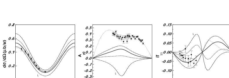
FIG. 1.: Differential cross section $d\sigma/d\Omega$, asymmetry $A_{y0}$ and vector polarization $iT_{11}$ for $pp\to d\pi^{+}$ as a function of scattering angle in the c.m.s. at $T_{p}=578MeV$ when the cut-off parameter $\Lambda$ and mixing one $\lambda$ varied simultaneously both in the deuteron wave function and in the $\pi NN$ vertex. The dashed ($\lambda=0.6;\Lambda=1$), solid ($\lambda=0.8;\Lambda=0.6$) and dot-dashed ($\lambda=1;\Lambda=0.6$) lines correspond to the Gross ${\cal W}{\cal F}{\cal D}$ [17]. The dot-dot-dashed line corresponds to the results with Locher’s ${\cal W}{\cal F}{\cal D}$ [16] ($\lambda=1;\Lambda=1$). The dots represent the partial-wave analysis by R. A. Arndt et al. [30]. The data are from [14, 15, 30]. All spin observables are in the Madison convention.

FIG. 2.: Spin correlations $A_{ii}$. Notation as in Fig.(1).

REFERENCES

[1]
K. M. Watson and K. A. Bruckner, Phys.Rev. 83 (1951) 1.
[2]
A. H. Rosenfeld, Phys.Rev. 96 (1954) 139.
[3]
S. Mandelstam, Proc.Roy.Soc.London Ser.A244 (1958) 491.
[4]
J. A. Niskanen, Nucl.Phys.A298 (1978) 417;
Phys.Lett.B71 (1977) 40; B79 (1978) 190.
[5]
A. M. Green and J. A. Niskanen, Nucl.Phys.B271 (1976) 503;
A. M. Green and M. E. Sainio, J.Phys. G: Nucl.Phys.4(1978)
1055.
[6]
T. Mizutani and D. Koltun, Ann.Phys. (N.Y.)109 (1977) 1.
[7]
A. S. Rinat, Nucl.Phys.A287 (1977) 399; A. S. Rinat,
Y. Starkand and E. Hammel, Nucl.Phys.A364 (1981) 486.
[8]
B. Blankleider and I. R. Afnan, Phys.Rev.C24 (1981) 1572.
[9]
T. Yao, Phys.Rev.B134 (1964) 454.
[10]
J. N. Chahoud, G. Russo and F. Selleri, Nuovo Cimento45
(1966) 38.
[11]
D. Schiff and J. Tran Than Van, Nucl.Phys.B5 (1968)
529.
[12]
G. W. Barry, Ann.Phys. (N.Y.)73 (1972) 482.
[13]
W. Grein. A. König, P. Kroll, M. P. Locher and and
A. varc, Ann.Phys. (N.Y.)153 (1984) 153.
[14]
M. P. Locher and and A. varc,
J. Phys. G: Nucl.Phys.11 (1985) 183.
[15]
M. P. Locher and and A. varc,
Few-Body Systems5 (1988) 59.
[16]
M. P. Locher and and A. varc,
Z. Phys. A - Atoms and Nuclei316 (1984) 55.
[17]
W. W. Buck and F. Gross, Phys.Rev.D20 (1979) 2361.
[18]
F. Gross, J. W. Orden, Karl Holinde, Phys.Rev.C45 (1992)
2094.
[19]
C. Itzykson, J. B. Zuber, Quantum Field Theory, McGraw-Hill, 1980.
[20]
C. Borrely, E. Leader and J. Soffer, Phys.Rep.59 (1980) 95.
[21]
J. Gunion, S. Brodsky, Phys.Rev.D8 (1973) 287.
[22]
J. Gunion, Phys.Rev.D10 (1974) 242.
[23]
E. Kazes, Nuovo Cim.13 (1959) 1226.
[24]
S.S. Schweber, H.A.Bethe and F. de Hoffmann,
Mesons and Fields, Row, Peterson and Company, 1955.
[25]
W. T. Nutt and C. M. Shakin,
Phys.Rev.C16 (1977) 1107; Phys.Lett.B69
(1977) 290.
[26]
R. Machleidt, K. Holinde and Ch. Elster, Phys.Rep.149
(1987) 1.
[27]
G. Höhler, F. Kaiser,E. Pietarinen,
Handbook of Pion-Nucleon Scattering12 (1979) 1.
[28]
A. König, P. Kroll, Nucl.Phys.A356 (1981) 354.
[29]
F. Foroughi, J. Phys. G: Nucl.Phys.8 (1982) 1345.
[30]
R. A. Arndt et al., Phys.Rev.C48 (1993) 1926.
[31]
Those with access to TELNET can run the SAID program with a link to
http://clsaid.phys.vt.edu
[32]
G. I. Lykasov, Phys. Part. Nuclei24 (1993) 59.
[33]
L. Ya. Glozman, V. G. Neudatchin and I. T. Obukhovsky,
Phys. Rev.C48 (1993) 389.
[34]
A. Kobushkin J. Phys. G: Nucl. Phys.19 (1993) 1993.
FIG. 1.:
Differential cross section , asymmetry and vector
polarization for as a function of scattering angle
in the c.m.s. at when the cut-off parameter and mixing
one varied simultaneously both in the deuteron wave function and in
the vertex. The dashed (), solid () and dot-dashed () lines correspond to the Gross
[17]. The dot-dot-dashed line corresponds to the
results with Locher’s [16] ().
The dots represent the partial-wave analysis by R. A. Arndt et al.
[30]. The data are from [14, 15, 30].
All spin observables are in the Madison convention.