Formation of correlations at short time scales and consequences on interferometry methods

Abstract

The formation of correlations due to collisions in an interacting nucleonic system is investigated shortly after a disturbance. Results from one-time kinetic equations are compared with the Kadanoff and Baym two-time equation with collisions included in second order Born approximation. A reasonable agreement is found for a proposed approximation of the memory effects by a finite duration of collisions. The formation of correlations and the build up time is calculated analytically for the high temperature and the low temperature limit. This translates into a time dependent increase of the effective temperature on time scales which interfere with standard fire ball scenarios of heavy ion collisions. The consequences of the formation of correlations on the two- particle interferometry are investigated and it is found that standard extracted lifetimes should be corrected downwards.

1 Introduction

To extract information about the space- time character of particle- emitting sources is one of currently much investigated tasks [1, 2]. The size of stars are found to be measurable by coincident photons [3]. In laboratory this method is used to analyse heavy ion reactions [4]. The two-particle correlation function carries the information about nuclear interaction and correlations in the emitting source [5, 6] and is given by the ratio of two - and single particle emission probability

$$R(P=p_{1}+p_{2},q=(p_{1}-p_{2})/2)+1={\Pi(p_{1},p_{2})\over\Pi(p_{1})\Pi(p_{2})}$$ (1)

which can alternatively be expressed by cross sections [7]. This two-particle correlation function can be written in terms of the the two-particle wave function $\varphi(q,r)$

$$R(P,q)+1=\int d^{3}rF_{p}(r)|\varphi(q,r)|^{2}$$ (2)

while the average of the single particle Wigner functions of the source is given by [8, 9]

$$F_{p}(r)={\int d^{3}R\,f(P/2,R+r/2,t^{>})\,f(P/2,R-r/2,t^{>})\over\left(\int d^{3}R\,f(P/2,R,t^{>})\right)^{2}}.$$ (3)

Here $f(p,r,t>)=\int\limits^{t^{>}}dt\,g(p,r-p(t^{>}-t)/m,t)$ is the phase-space Wigner distribution of particles of momenta $p$ at position $r$ at some time $t^{>}$ after emission with probability $g$. A rigorous derivation of this formula with the discussion of the necessary neglects has been given in [1] for the case of initially uncorrelated particles $|\varphi(p,r)|^{2}\propto 1\pm\cos(rq)$ corresponding to bosons/fermions. Eq. (3) is well suited for simulation of heavy ion reactions where the one-time distribution function $f({\bf r,p},t)$ is then determined by solving appropriate kinetic equations (BUU) or simulating equation of motions (QMD). While most current codes rely on the quasiclassical Boltzmann equation including Pauliblocking effects, a quantum two-time theory for the time-evolution of real time Green’s functions $G({\bf r,p},t,t^{\prime})$ has been developed using the Schwinger-Keldysh formalism already 30 years ago. The quantum image of the classical Boltzmann equation is usually referred to as the Kadanoff-Baym (KB) equations [10]. These equations have often been considered too complicated to solve numerically in the past. However, several numerical applications exist now [11].

These kinetic equations describe different relaxation stages. During the very fast first stage, correlations imposed by the initial preparation of the system are decaying [12, 13]. These are contained in off-shell or dephasing processes described by two-time propagators. During this stage of relaxation the quasiparticle picture is established [14, 15]. After this very fast process the second state develops during which the one-particle distribution relaxes towards the equilibrium value with a relaxation time. This is characterized by a nonlocal kinetic equation in agreement with the virial correction to the approached equation of state [16]. We will focus on the first stage which is related to the formation of correlations and will find a measurable effect on the two-particle correlation function. The extracted lifetimes are shown to be too high if one ignores this transient time effects. This can be considered to belong to the initial state correlations. While in [17, 18] the initial state correlations are assumed to be of equilibrium type and discussed by density and temperature dependence we like to investigate here a nonequilibrium effect which consists in the fact that correlations need a specific time to be build up.

The formation of correlations is connected with an increase of the kinetic energy or equivalently the build up of correlation energy. This is due to rearrangement processes which let decay higher order correlation functions until only the one - particle distribution function relaxes.

2 Kinetic description

The time dependence of the kinetic energy as a one-particle observable will be investigated within the kinetic theory. This can only be accomplished if we employ a kinetic equation which leads to total energy conservation. It is immediately obvious that the ordinary Boltzmann equation cannot be appropriate for this purpose because the kinetic energy is in this case an invariant of the collision integral and constant in time. In contrast, we have to consider non-Markovian kinetic equations of Levinson type [19, 20], which account for the formation of two particle correlations and which conserves the total energy [21] [22, 23, 24]

$$\frac{\partial}{\partial t}f_{a}(t)=\frac{2s_{a}}{\hbar^{2}}\sum\limits_{b}s_{b}\int\frac{dpdq}{(2\pi\hbar)^{6}}V_{\rm D}^{2}(q)$$

$$\times\int\limits_{t_{0}}^{t}d\bar{t}\,\exp\left\{-{t-\bar{t}\over\tau_{g}}\right\}\,{\rm cos}\left\{\frac{1}{\hbar}(t-\bar{t})\Delta_{E}\right\}\left\{f^{\prime}_{a}f^{\prime}_{b}\bar{f}_{a}\bar{f}_{b}-f_{a}f_{b}\bar{f}^{\prime}_{a}\bar{f}^{\prime}_{b}\right\},$$ (4)

where $\Delta_{E}={k^{2}\over 2m_{a}}+{p^{2}\over 2m_{b}}-{(k-q)^{2}\over 2m_{a}}-{(p+q)^{2}\over 2m_{b}}$ denotes the energy difference between initial and final states. The retardation of distributions, $f_{a}(k,\bar{t})$, $f^{\prime}_{a}(k-q,\bar{t})$ etc., is balanced by the quasiparticle damping $\tau_{g}$ and $\bar{f}=1-f$, the free particle dispersion $E=p^{2}/2m$ and the spin-isospin degeneracy $s$. The distribution functions are normalized to the density as $\int{dp\over(2\pi\hbar)^{3}}f(p)=n/s$.

The Boltzmann collision integral is obtained from equation (4) if: (i) One neglects the time retardation in the distribution functions, i.e. the memory effects. This would lead to gradient contributions to the kinetic equation which can be shown to be responsible for the formation of high energy tails in the distribution function [25, 26] and virial corrections [27, 28, 16]. This effect will be established on the second stage of relaxation. (ii) The finite initial time $t_{0}$ is set equal to $-\infty$ corresponding to what is usually referred to as the limit of complete collisions. This energy broadening or off-shell behavior in (4) is exclusively related to the spectral properties of the one-particle propagator and therefore determined by the relaxation of two-particle correlation.

Since we are studying the very short time region after the initial disturbance we can separate the one-particle and two-particle relaxation. On this time scale the memory in the distribution functions can be neglected $\bar{f}_{a}(\bar{t})=f_{a}(0)$, $\exp\left\{-{t-\bar{t}\over\tau_{g}}\right\}=1$ but we will keep the spectral relaxation implicit in the off-shell $\cos$-function of (4).

The eq. (4) can be integrated with respect to time and the resulting equation for $f(t)$ represents the deviation of Wigner’s distribution from its initial value, $f_{a}(t)=f_{a}(0)+\delta f_{a}(t)$, and reads

$$\delta f_{a}(t) = 2\sum\limits_{b}\int\frac{dpdq}{(2\pi\hbar)^{6}}V^{2}_{\rm D}(q){1-\cos\left\{{1\over\hbar}t\Delta_{E}\right\}\over\Delta_{E}^{2}}\left\{f^{\prime}_{a}f^{\prime}_{b}\bar{f}_{a}\bar{f}_{b}-f_{a}f_{b}\bar{f}^{\prime}_{a}\bar{f}^{\prime}_{b}\right\}.$$ (5)

This formula shows how the two-particle and the single-particle concepts of the transient behavior meet in the kinetic equation. The right hand side describes how two particles correlate their motion to avoid the strong interaction regions. Since the process is very fast, the on-shell contribution to $\delta f_{a}$, proportional to $t/\tau$, can be neglected in the assumed time domain and the $\delta f$ has the pure off-shell character as can be seen from the off-shell factor $\Delta_{E}^{-2}\left(1-\cos\left\{{1\over\hbar}t\Delta_{E}\right\}\right)$. The off-shell character of mutual two-particle correlation is thus reflected in the single particle Wigner’s distribution.

The very fast formation of the off-shell contribution to Wigner’s distribution has been found in numerical treatments of Green’s functions [29, 30]. Once formed, the off-shell contributions change in time with the characteristic time $\tau$, i.e., following the relaxation (on-shell) processes in the system. Accordingly, the formation of the off-shell contribution signals that the system has reached the state the evolution of which can be described by the nonlocal Boltzmann equation [16], i.e., the transient time period has been accomplished.

From Wigner’s distribution (5) one can readily evaluate the increase of the kinetic energy

$$E^{\rm static}_{\rm corr}(t) = -\sum_{ab}\int\frac{dkdpdq}{(2\pi\hbar)^{9}}V^{2}_{\rm D}(q)\frac{1-\cos\left\{{1\over\hbar}t\Delta_{E}\right\}}{\Delta_{E}}f^{\prime}_{a}f^{\prime}_{b}\bar{f}_{a}\bar{f}_{b}.$$ (6)

This expression holds for general distributions $f_{a}$. We choose a model of two initially counter - flowing streams of nuclear matter and plot in figure 1 the time evolution of the kinetic energy and the correlation.

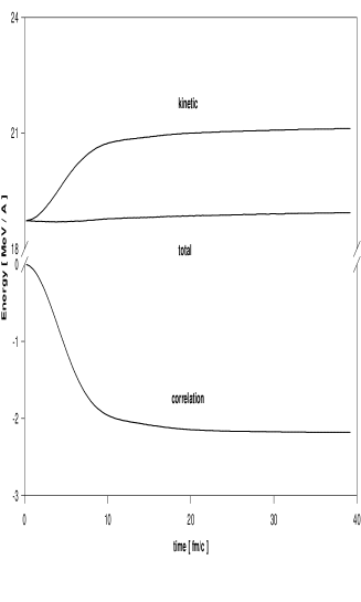
Figure 1: The time evolution of the correlation and kinetic energy for two initially counter -flowing streams of nuclear matter with density and temperature $n_{1}=n_{o}/60\quad T_{1}=0.5$ MeV and $n_{2}=n_{o}/20\quad T_{2}=0.1$ MeV moving with relative velocity of $1\hbar/fm$ which corresponds to a collision energy of $21$ MeV/n. In this case the correlation time $\tau_{c}=9fm/c$. The equilibrated temperature is here (neglecting correlations) $T=11.6$ MeV and a Gauß type of potential has been used.

This build up of correlations is found to be independent of the form of the initial distribution. If for example we choose a (equilibrium) Fermi distribution as the initial distribution a build up of correlations will occur as well. This is due to the fact that the spatial correlations relate in momentum space to excitations, resulting in a distribution looking somewhat like a Fermi-distribution but with a temperature higher than that of the initial uncorrelated Fermi-distribution.[31]

3 The formation of correlations

We start now to calculate the observed increase of kinetic energy analytically. As a first example we shall consider a Yukawa-type potential of the form $V_{\rm Y}(r)={g_{ab}\over r}{\rm e}^{-\kappa r}$ where in nuclear physics applications $g_{ab}$ is the coupling and $\kappa$ the effective range of potential given by the inverse mass of interchanging mesons. As a second example we shall use a Gauß-type potential $V_{G}(r)=V_{0}{\rm e}^{-(r/\eta)^{2}}$ which has been used in nuclear physics applications[32, 31] with $\eta=0.57{\rm fm}^{-3}$ and $V_{0}=-453$ MeV.

The high temperature limit of the time dependence of the correlation energy can be calculated analytically [33, 15]. The low temperature value is of special interest, because it leads to a natural definition of the build up of correlations. One obtains

$${\partial\over\partial\,t}E_{\rm corr} = -\frac{1}{2}m^{4}p_{f}\langle{V^{2}\over\cos{\frac{\theta}{2}}}\rangle\tilde{I}_{f}$$ (7)

with standard notation of angular integrals [34] and finds the time dependence of the correlation energy [33]

$$E^{low}_{\rm corr}(t)-E_{\rm corr}^{low}(0)=E_{\rm corr}^{low}(1+\frac{1}{3}({\epsilon_{f}+\epsilon_{c}\over\pi T})^{2})^{-1}$$ (8)

$$\times \left\{1-\frac{1}{x}\sin(x)+\left({\epsilon_{f}+\epsilon_{c}\over\pi T}\right)^{2}\left(\frac{1}{3}+\left[\frac{1}{x}\sin(x)\right]^{\prime\prime}\right)\right\}$$

with $x=2{\epsilon_{f}+\epsilon_{c}\over\hbar}t$ and the equilibrium correlation energy $E_{\rm corr}^{\rm low}$ for the Yukawa- or Gauß- potential reads [33]

$$E_{\rm corr} = \frac{1}{6}s_{1}s_{2}\tilde{\epsilon}_{f}\left(T^{2}+\frac{1}{3}\left({4\tilde{\epsilon}_{f}\over\pi}\right)^{2}\right)\left({m\over\hbar^{2}}\right)^{4}\left\{\matrix{{g^{2}\over 2\kappa^{3}\pi^{2}}\left(\arctan{\frac{1}{b_{l}}}+{b_{l}\over 1+b_{l}^{2}}\right)\quad Yuk.\cr{V_{0}^{2}\eta^{5}\over 2\sqrt{2\pi}}{\rm erf}({p_{f}\eta\sqrt{2}\over\hbar})\quad\mbox{\it Gau\ss{}}}\right.$$

where $\tilde{\epsilon}_{f}={\epsilon_{f}+\epsilon_{c}\over 4}$ and $b_{l}={\hbar\kappa\over 2p_{f}}$. The best choice for cut-off we found $\epsilon_{c}\approx\epsilon_{f}$. We see that the correlation energy is built up and oscillates around the equilibrium value damped with $t^{-1}$ in time. We now define the build up time $\tau_{c}$ as the time where the correlation energy has reached its first maximum. This time is given by $\tau_{c}\approx{\hbar\over\epsilon_{F}}$.

We assert here that the result (8) is valid for any binary interaction. We could use Born or $T$-matrix approximation and the same time dependence but different $E_{\rm corr}^{low}$ would result. This correlation time limits the validity of quasiparticle picture which is established at times greater than $\tau_{c}$ [15]. Incidentally, in the early 1950s the criterion $\hbar/k_{B}T<\tau$ was supposed to limit the validity of the Landau Fermi-liquid theory for metals [35]. Later it was shown by Landau that this criterion is irrelevant and he proposed the correct criterion $\tau>\hbar/\epsilon_{F}$.

In order to illustrate the weak temperature dependence of $\tau_{c}$ we plot in figure 2 (thick lines) results from the solution of the Kadanoff and Baym equations for a fixed chemical potential of $37.1$ MeV and for three different temperatures. The figure shows the increase of the kinetic energy (equivalent to the decrease of correlation energy) with time. The KB results are compared with those from approximation (8). One sees that the agreement is good initially while correlations are built up. At low temperatures the oscillations discussed above are obvious in the approximate results while the KB calculations only show a slight overshoot at the lowest temperatures. We believe that the discrepancy is due to the damping that is neglected in (5).

Figure 2: The formation of correlation plotted as an increase of the kinetic energy with time for temperatures $1,10,40$ MeV. The chemical potential is fixed to $37.1$ MeV which corresponds to densities $0.16,0.18,0.35{\rm fm}^{-3}$ . The thick lines show results from KB calculations while the thin lines are approximate values via formula (8). The equilibrium correlation energy was chosen to be equal to the KB result. The oscillations are overestimated by the approximate formula. For $T=40$ MeV we plotted also the high temperature approximate value [33] as thin solid line. The built up of correlations is too fast.

We can give a Pad e formula for the increase of kinetic energy which interpolates the results of K/B equation within the temperature range up to Fermi energy $\zeta_{\rm K/B}$ and the analytical result (8) signed $\zeta(t)$

$$\zeta_{\rm K/B}(t) = {E_{\rm corr}(t)\over E_{\rm corr}(\infty)}=1-{{1.5225\,\left(1-\cos(0.7337\,{x})+\sin(0.6568\,{x})\right)}\over{{{\rm e}^{0.5469\,{x}}}\,{x}}}$$

$$\zeta(t) = 1-{\sin(x)\over x}$$ (10)

with $x=4\epsilon_{F}t/\hbar$. The $\zeta_{\rm K/B}$ is a smooth curve through $\zeta(t)$. As we pointed out above, this result is universal for any binary interaction approximation. Therefore we can adopt this scaling as a universal scaling of the one-particle Wigner distribution. Provided we have solved any local Markovian kinetic equation like BUU, we can simply multiply the obtained Wigner function by the time dependent factor (3) in order to incorporate the transient time effect approximately. Since we fixed this factor to the observable kinetic energy, we expect to have correctly described the energy variables.

4 Application to interferometry

Now we employ the found scaling of short time effects to the formula (3) and adopt a space-time source parameterization of

$$g(p,r,t)=\rho_{0}\Theta(r)\Theta(R_{s}-r)\Theta(t)p{\rm e}^{-{p^{2}\over 2mT}}{\rm e}^{-t/\tau}\zeta(t)$$ (11)

with the radius $R_{s}$ and lifetime $\tau$ of the source and the scaling $\zeta(t)$ of (3). Without center of mass momentum $P$ the correlation function becomes independent of lifetime and collapse to the standard interferrometry result [36]

$$R(0,q)+1={3\over 4\pi R_{s}^{3}}\int\limits_{0}^{2R_{s}}d^{3}r|\varphi(q,r)|^{2}\left(1-\frac{3}{4}{r\over R_{s}}+\frac{1}{16}\left({r\over R_{s}}\right)^{3}\right).$$ (12)

Considering the momentum dependence and assuming initially free particles $|\varphi(p,r)|^{2}\propto 1\pm\cos(rq)$ we obtain a separable representation

$$R(P,q)+1=1\pm\Psi(q.R_{s})\Pi(\zeta,q.p,\tau)$$ (13)

with

$$\Psi(x) = {3\over 2x^{6}}\left((-3+3x^{2}-2x^{3}+4x^{4})\cos(2x)+(-6x-6x^{3}-4x^{4})\sin(2x)\right)$$

and

$$\Pi(\zeta,q.p/2m,\tau)={\int\limits_{0}^{\infty}dtdt^{\prime}{\rm e}^{-(t+t^{\prime})/\tau}\zeta(t)\zeta(t^{\prime})\cos(q.p(t^{\prime}-t)/2m)\over\left(\int\limits_{0}^{\infty}dt{\rm e}^{-t/\tau}\zeta(t)\right)^{2}}.$$ (15)

While the first factor $\Psi$ gives the dependence of the correlation function on the source size, the second factor contains the effect of finite lifetimes. The result without transient time effects is that with increasing lifetime the correlation functions are diminished [9]. One gets for $\zeta=1$ just

$$\Pi_{0}(1,q.p,\tau)={1\over 1+(q.p\tau/2m)^{2}}.$$ (16)

We can write the analytical result for (15) with $\zeta(t)$ from (3)

$$\Pi(a,c,\tau) = \left(4\,{{\left({{-2\,a\,\tau}\over{1+{c^{2}}\,{{\tau}^{2}}}}+\arctan(\left(a-c\right)\,\tau)+\arctan(\left(a+c\right)\,\tau)\right)}^{2}}\right.$$ (17)

$$+ \left.{{\left({{-4\,a\,c\,{{\tau}^{2}}}\over{1+{c^{2}}\,{{\tau}^{2}}}}-\log(1+{{\left(a-c\right)}^{2}}\,{{\tau}^{2}})+\log(1+{{\left(a+c\right)}^{2}}\,{{\tau}^{2}})\right)}^{2}}\right)$$

$$/ (16\,{{\left(a\,\tau-\arctan(a\,\tau)\right)}^{2}})$$

with $c=4\epsilon_{F}/\hbar$ and $a=q.p/2m$. Figure 3 shows the influence of the transient time effect on the correlation function. We have plotted conveniently the ratio of reduced correlation functions $\Pi$ of (15) with short time dynamics to $\Pi_{0}$ of (16) without short time dynamics.

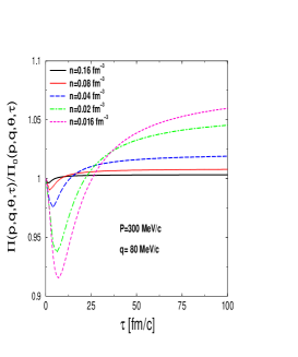
Figure 3: The ratio of correlation function $\Pi$ of (15) with short time dynamics to $\Pi_{0}$ of (16) without short time dynamics versus lifetime of the source.

We recognize that there is a suppression for smaller lifetimes. Since the effect of lifetime $\tau$ itself lowers the correlation function we can state that the extracted lifetimes from experiments are too high if short time or transient time effects are neglected. For higher lifetimes this effect is opposite. The extracted lifetimes from experiment should be too low. Interesting is the density dependence. While first with decreasing density the lowering/enhancement shifts to higher lifetimes, there is a critical density where we have only suppression. It is found to be around $0.0036{\rm fm}^{-3}$.

Due to the found universal scaling this effect is important in any recent simulation of BUU- type since the transient time effect of formation of correlations and therefore increase of kinetic energy has not been considered so far. For moleculardynamical methods this is in principle included but buried in artificial initial correlations due to the numerical set up. For a comparison between the kinetic and MD simulation see [15].

5 Summary

The gradient approximation of the kinetic equation in second order Born approximation is investigated. A finite duration approximation of the non Markovian collision integral is proposed which follows from time dependent Fermi’s Golden Rule and which is in good agreement with the numerical solution of complete Kadanoff and Baym equation.

The build up time of correlations is investigated and it is found that the low temperature value is universal for any approximation at the binary collision level. It is shown that the formation time of correlations is nearly determined by the ratio of $\hbar$ to the transfer energy which can be considered as an analogue to the uncertainty principle.

A universal scaling is formulated which allows to map the Wigner function of Markovian simulation to a result including the transient time effect. As a consequence the influence to interferrometry methods is discussed. It is found that the extracted lifetimes from experiment should be too large for lower lifetimes and too small for higher values depending on the freeze out-density if transient time effects are neglected.

References

References

- [1] G. F. Bertsch, P. Danielewicz, and M. Herrmann. Phys. Rev. C, 49:442, 1994.
- [2] D. H. Boal, C. K. Gelbke, and B. K. Jennings. Rev. Mod. Phys., 62:553, 1990.
- [3] R. Hanbury-Brown and R. Q. Twiss. Nature (London), 178:1046, 1956.
- [4] J. Pochodzalla and et. al. Phys. Rev. C, 35:1695, 1987.
- [5] S. E. Koonin. Phys. Lett. B, 70:43, 1977.
- [6] W. G. Gong and et. al. Phys. Rev. C, 43:1804, 1991.
- [7] W. Bauer. Nucl. Phys. A, 471:604, 1987.
- [8] S. Pratt and M. B. Tsang. Phys. Rev. C, 36:2390, 1987.
- [9] W. G. Gong, W. Bauer, C. K. Gelbke, and S. Pratt. Phys. Rev. C, 43:781, 1991.
- [10] L. P. Kadanoff and G. Baym. Quantum Statistical Mechanics. Benjamin, New York, 1962.
- [11] H.S. Köhler. Phys. Rev. E, 53:3145, 1996.
- [12] N. N. Bogoljubov. J. Phys. (USSR), 10:256, 1946. transl. in Studies in Statistical Mechanics, Vol. 1, editors D. de Boer and G. E. Uhlenbeck (North-Holland, Amsterdam 1962).
- [13] M. Bonitz and et. al. J. Phys.: Condens. Matter, 8:6057, 1996.
- [14] P. Lipavský, F. S. Khan, A. Kalvová, and J. W. Wilkins. Phys. Rev. B, 43(8):6650, 1991.
- [15] K. Morawetz, V. Špička, and P. Lipavský. Formation of correlations in plasma at short time scales. Phys. Lett. A in press.
- [16] V. Špička, P. Lipavský, and K. Morawetz. Phys. Lett. A, 240:160, 1998.
- [17] T. Alm. PhD thesis, Universität Rostock, 1992. report GSI-93-07,Darmstadt.
- [18] T. Alm, G. Röpke, and M. Schmidt. Phys. Lett. B, 301:170, 1993.
- [19] I. B. Levinson. Fiz. Tverd. Tela Leningrad, 6:2113, 1965.
- [20] I. B. Levinson. Zh. Eksp. Teor. Fiz., 57(2):660, 1969. [Sov. Phys.–JETP 30, 362 (1970)].
- [21] K. Morawetz. Phys. Lett. A, 199:241, 1995.
- [22] A. P. Jauho and J. W. Wilkins. Phys. Rev. B, 29(4):1919, 1984.
- [23] K. Morawetz, R. Walke, and G. Röpke. Phys. Lett. A, 190:96, 1994.
- [24] H. Haug and A. P. Jauho. Springer, Berlin Heidelberg, 1996.
- [25] K. Morawetz and G. Röpke. Phys. Rev. E, 51(5):4246, 1995.
- [26] V. Špička and P. Lipavský. Phys. Rev. B, 52(20):14615, 1995.
- [27] V. Špička, P. Lipavský, and K. Morawetz. Phys. Rev. B, 55(8):5084, 1997.
- [28] V. Špička, P. Lipavský, and K. Morawetz. Phys. Rev. B, 55(8):5095, 1997.
- [29] P. Danielewicz. Ann. Phys. (NY), 152:305, 1984.
- [30] H. S. Köhler. Phys. Rev. C, 51:3232, 1995.
- [31] H.S. Köhler. Phys. Rev. C, 51:3232, 1995.
- [32] P. Danielewicz. Ann. Phys. (NY), 152:239, 1984.
- [33] K. Morawetz and H. S. Koehler. Phys. Rev. C, 1997. sub.
- [34] H. Smith and H. Hojgaard-Jensen. Clarendon Press, Oxford, 1989.
- [35] R. Peierls. Quantum Theory of Solids. Oxford University Press, London, 1955.
- [36] B. K. Jennings, D. H. Boal, and J. C. Shillcock. Phys. Rev. C, 33:1303, 1986.