Consequences of coarse grained Vlasov equations

Abstract

The Vlasov equation is analyzed for coarse grained distributions resembling a finite width of test-particles as used in numerical implementations. It is shown that this coarse grained distribution obeys a kinetic equation similar to the Vlasov equation, but with additional terms. These terms give rise to entropy production indicating dissipative features due to a nonlinear mode coupling The interchange of coarse graining and dynamical evolution is discussed with the help of an exactly solvable model for the selfconsistent Vlasov equation and practical consequences are worked out. By calculating analytically the stationary solution of a general Vlasov equation we can show that a sum of modified Boltzmann-like distributions is approached dependent on the initial distribution. This behavior is independent of degeneracy and only controlled by the width of test-particles. The condition for approaching a stationary solution is derived and it is found that the coarse graining energy given by the momentum width of test particles should be smaller than a quarter of the kinetic energy. Observable consequences of this coarse graining are: (i) spatial correlations in observables, (ii) too large radii of clusters or nuclei in self-consistent Thomas-Fermi treatments, (iii) a

structure term in the response function resembling vertex correction correlations or internal structure effects and (iv) a modified centroid energy and higher damping width of collective modes.

]

I Introduction

The Boltzmann kinetic equation is a successfully used dynamical model to describe heavy ion collisions and multifragmentation up to intermediate energies [1, 2, 3, 4, 5, 6, 7, 8, 9, 10, 11]. The scattering is added to the Vlasov equation either by the relaxation time [12, 13, 14, 15, 16] or by scattering integrals of the Boltzmann-type [4, 7, 16, 17, 18, 19, 20, 21, 22] or their nonlocal extensions [23, 24, 25] in the same way as it was done in the Landau-Vlasov equation for hot plasmas. All these simulation have in common that the motion of particles between collisions are covered by Hamilton equations or the Vlasov kinetic equation with a selfconsistent potential.

Even within collisionless Vlasov codes the onset of fragmentation is described [26, 27, 28]. The use of selfconsistent Vlasov equation is not restricted to nuclear collisions but has been applied successfully for collisions of ions with metal clusters [29, 30, 31]. Despite the fact that the Vlasov equation is a reversible kinetic equation and the initial configuration should be retained after a long enough calculation, fragmentation and energy dissipation is observed. Obviously this is due to the fact that the Poincaré time is much larger than the time where the phase space is filled by various trajectories. Therefore one can consider superficially this spreading as an irreversible process in the sense of entropy production. Nevertheless, the underlying dynamics is reversible.

The numerical implementation of Vlasov codes demands a certain coarse graining of the space and momentum coordinates. This numerical uncertainty is quite sufficient to generate genuine dissipation and entropy production. This fact has been investigated in [32] and will be considered in detail within this paper. It has been argued that the errors due to numerically coarse graining accumulate diffusively. We will demonstrate that these errors will lead to a unique equilibration of Vlasov equation. While the diffusion itself is less effected, the coarse graining leads to a different dynamical evolution and has consequences for the extraction of damping rates from Vlasov-type simulations.

Theoretically one can derive kinetic equations by phase-space averaging of the Liouville equation which itself is exactly of Vlasov type [33]. The resulting collision integrals represent two different approximations of the nonequilibrium dynamics: (i) The truncation of coupling to higher order correlations (hierarchy) and (ii) The smoothing procedure which translates the fluctuating stochastic equation into a kinetic equation for the smoothed distribution function. This latter procedure is sometimes also called coarse graining. For the discussion of appropriate collision integrals also in the quantum case see [34]. Here we will focus on a detailed analysis of consequences of coarse graining.

The idea used here dates back to the work of Gibbs and Ehrenfest [35, 36]. They suggested to coarse grain the entropy definition by a more rough distribution function

$$f(p,r,t)={1\over\Delta(p,r)}\int\limits_{\Delta(p,r)}f_{\delta}(p^{\prime},r^{\prime},t)dp^{\prime}dr^{\prime}.$$ (1)

The physical meaning consists in the fact that any observable is a mean value of an averaging about a certain area in phase space. It was shown that the entropy with this coarse grained distribution increases [37]. This means that in a closed system the entropy can rise if we average the observation about small phase space cells.

The interpretation is that other phase space points can enter and leave the cell which is not compensated. A phase space mixing occurs [37] since the two limits cannot be interchanged, i.e. the thermodynamic limit and the limit of vanishing phase space cell. The coarse graining of Ehrenfest can be observed if the thermodynamical limit is carried out first and the limit of small phase space cells afterwards. It solves therefore not the problem of entropy production, but gives an interesting aspect to entropy production by coarse grained observations [37].

In this paper we like to investigate three questions:

• Which kinetic equation is really solved numerically if the Vlasov equation is implemented in numerics?

• What are the properties of this kinetic equation, especially which kind of dissipative features appear ?

• What are the consequences to practical applications, e.g. damping of giant resonances and binding energies?

The outline of the paper is as follows. Next we derive the kinetic equation which is obeyed by the coarse grained distribution function. Then in chapter III we discuss the entropy production. We demonstrate with the help of two exactly solvable models that this entropy production is due to mixing, i.e. a mode coupling and not simply by spreading of Gaussians. The solution of the stationary Vlasov equation is then presented in chapter IV. We will find that the stationary solution can be represented as an infinite sum of modified Boltzmann distributions. This expansion shows the unique character of time evolution which is only determined by the initial distribution. In chapter V we discuss consequences of this result: (i) The thermodynamics becomes modified by spatial correlations. The selfconsistency leads to a modified Thomas- Fermi equation lowering the binding energy, (ii) the structure factor shows a substructure similar as obtained from vertex corrections and (iii) the damping width of collective resonances is shown to be larger by coarse graining. While the centroid energy is smaller by momentum coarse graining it increases by spatial coarse graining.

II Coarse grained Vlasov equation

The origin of the coarse graining may be the numerical implementation or the use of averaged distribution functions instead of the fluctuating one. To illustrate the method we examine the quasi-classical Vlasov equation and show which equation is really solved if one is forced, by numerical reasons, to use coarse graining. It will become clear shortly that instead of Vlasov equation a modified kinetic equation is solved when coarse graining is present. The quantum mechanical or TDHF equation can be treated in analogy. We start from the Vlasov equation

$${\partial\over\partial\,t}f_{\delta}(prt)+{p\over m}{\partial\over\partial\,r}f_{\delta}(prt)-{\partial\over\partial\,r}V_{\delta}(r,t){\partial\over\partial\,p}f_{\delta}(prt)=0$$ (2)

which solution can be formally represented as an infinite sum of exact test-particles

$$f_{\delta}(prt)=\sum\limits_{i=1}^{\infty}\delta(r-R_{i}(t))\,\delta(p-P_{i}(t))$$ (3)

where the test-particle positions and momenta evolve corresponding to the Hamilton equations ${\dot{R}_{i}(t)}=P_{i}/m$ and ${\dot{P}_{i}(t)}=-\partial_{R}V(R_{i}(t))$. In the following we understand $p,r,P$ and $R$ as vectors and suppress their explicit notation.

For the mean-field term $V_{\delta}$ we assume a Hartree approximation given by a convolution of the density with the two-particle interaction $V_{0}$

$$V_{\delta}(r,t)=\int dr^{\prime}V_{0}(r-r^{\prime})\int{dp^{\prime}\over(2\pi\hbar)^{3}}f_{\delta}(p^{\prime}r^{\prime}t).$$ (4)

In practice all numerical calculations use two assumptions : (i) The infinite number of test-particles is truncated by a finite value. (ii) The used test particle has a finite width due to numerical errors and/or smoothing demand of the procedure. While in [38, 39, 40] was discussed that the approximation (i) leads to a Boltzmann-like collision integral, the approximation (ii) will deserve further investigations. Especially, we will show that the finite width of test-particles leads to a coarse graining and a dissipation forcing the system to a Boltzmann- like distribution. This is even valid with infinite numbers of test-particles. Therefore we consider the effect of coarse graining as the most determining one for one-body dissipation.

The finite width of test particles can be reproduced most conveniently by a convolution of the exact solution (3) with a Gaussian $g_{a}(x)=(2\pi\sigma_{a}^{2})^{-1.5}{\rm exp}(-x^{2}/(2\sigma_{a}^{2}))$ resulting in the coarse grained distribution function $f$

$$f(prt) = \{f_{\delta}\}_{g}$$ (5)

$$= \int{dp^{\prime}\over(2\pi\hbar)^{3}}dr^{\prime}g_{r}(r-r^{\prime})g_{p}(p-p^{\prime})f_{\delta}(p^{\prime}r^{\prime}t)$$ (6)

$$= \sum\limits_{i=1}^{\infty}g_{r}(r-R_{i}(t))g_{p}(p-P_{i}(t)).$$ (7)

To answer the question which kind of kinetic equation describes this smoothed distribution function, the kinetic equation for (7) is derived from (2) by convolution with a Gaussian. The equation for general coarse grained mean-fields has been already derived in [40]. In order to make the physical content more explicit we calculate the different terms explicitly and present the coarse grained kinetic equation. The free drift term ${p\over m}\partial_{r}f_{\delta}$ takes the form after convolution

$$\{{p\over m}\partial_{r}f_{\delta}\}_{g}={p\over m}{\partial\over\partial\,r}f(prt)+{\sigma_{p}^{2}\over m}{\partial\over\partial\,r}{\partial\over\partial\,p}f(prt)$$ (8)

which is established by partial integration. We see that the free streaming is modified by an additional resistive term which will give dissipative features.

The mean-field term takes the form

$$\{{\partial\over\partial\,r}V_{\delta}(r){\partial\over\partial\,p}f_{\delta}(prt)\}_{g} = {\partial\over\partial\,p}\{{\partial\over\partial\,r}V_{\delta}(r)f_{\delta}(prt)\}_{g}$$ (9)

$$= {\partial\over\partial\,p}\{\{{\partial\over\partial\,r}V_{\delta}(r)f_{\delta}(prt)\}_{g_{r}}\}_{g_{p}}.$$ (10)

The space convolution with $g_{r}$ is performed using the relation [41]

$$\{AB\}_{g}=\{A\}_{g}\rm{exp}(\sigma_{r}^{2}{\stackrel{{\scriptstyle\leftarrow}}{{\partial}}}_{r}{\stackrel{{\scriptstyle\rightarrow}}{{\partial}}}_{r})\{B\}_{g}$$ (11)

with the result

$${\partial\over\partial\,p}\{{\partial\over\partial\,r}V(r,t)\exp(\sigma_{r}^{2}{\stackrel{{\scriptstyle\leftarrow}}{{\partial}}}_{r}{\stackrel{{\scriptstyle\rightarrow}}{{\partial}}}_{r})\{f_{\delta}(prt)\}_{g_{r}}\}_{g_{p}}.$$ (12)

$V(r,t)$ is the mean-field calculated with the space and momentum coarse grained distribution $f$ instead of $f_{\delta}$, via (4) which can be seen as

$$V(r,t) = \{V_{\delta}(r,t)\}_{g_{r}}=\int dr^{\prime\prime}V_{0}(r^{\prime\prime})\int dr^{\prime}g_{r}(r-r^{\prime\prime}-r^{\prime})$$ (13)

$$\times \int{dp^{\prime}\over(2\pi\hbar)^{3}}f_{\delta}(p^{\prime},r^{\prime},t)$$ (14)

$$= \int dr^{\prime\prime}V_{0}(r^{\prime\prime})\int dr^{\prime}g_{r}(r-r^{\prime\prime}-r^{\prime})$$ (15)

$$\times \int{dp^{\prime}\over(2\pi\hbar)^{3}}\int{dp\over(2\pi\hbar)^{3}}g_{p}(p-p^{\prime})f_{\delta}(p^{\prime},r^{\prime},t)$$ (16)

$$= \int dr^{\prime\prime}V_{0}(r^{\prime\prime})\int{dp\over(2\pi\hbar)^{3}}f(p,r-r^{\prime\prime},t)$$ (17)

where the last equality shows the invariance of particle density due to coarse graining. The momentum convolution with the Gaussian is then performed in (12) to yield the momentum and space coarse distribution function $f$. We like to point out that the test-particle method would lead to a further folding of the mean-field potential if it is read off from a finite grid [38].

The coarse grained Vlasov equation reads now

$${\partial\over\partial\,t}f(prt) + {p\over m}{\partial\over\partial\,r}f(prt)+{\sigma_{p}^{2}\over m}{\partial\over\partial\,r}{\partial\over\partial\,p}f(prt)$$ (18)

$$- {\partial\over\partial\,r}V(r,t)\exp(\sigma_{r}^{2}{\stackrel{{\scriptstyle\leftarrow}}{{\partial}}}_{r}{\stackrel{{\scriptstyle\rightarrow}}{{\partial}}}_{r}){\partial\over\partial\,p}f(prt)=0.$$ (19)

This equation is the main result of this chapter and represents the Vlasov equation for the coarse grained distributions and should be compared with the Husimi representation of [40]. While the distribution function is exactly the Husimi representation of the Wigner function the corresponding coarse grained kinetic equation was not given before.

Equation (19) represents the kinetic equation which is really solved numerically if the Vlasov equation is attempted to be solved. The coarse graining leads to two additional contributions besides the original Vlasov equation. We will see that this causes just the dissipative like features. While we will continue now and investigate (19) more closely, in appendix A the question is addressed how the underlying dynamics is modified by coarse graining. We find that in principle the coarse grained equation can be mapped to the original Vlasov equation if one defines new testparticles with modified dynamical equations by a modified potential. The relation between the original and the modified potential appears just as the inverse folded mean field potential which is the opposite relation than presented in [38, 39, 40].

III Entropy production

To analyze the dissipative feature we rewrite (19) into

$${\partial\over\partial\,t}f(prt)+{p\over m}{\partial\over\partial\,r}f(prt)-{\partial\over\partial\,r}V(r,t){\partial\over\partial\,p}f(prt)=I_{\rm diss}$$ (20)

with the one-body (collision integral like) term

$$I_{\rm diss} = -{\sigma_{p}^{2}\over m}{\partial\over\partial\,r}{\partial\over\partial\,p}f(prt)$$ (21)

$$+ {\partial\over\partial\,r}V(r,t)(\exp(\sigma_{r}^{2}{\stackrel{{\scriptstyle\leftarrow}}{{\partial}}}_{r}{\stackrel{{\scriptstyle\rightarrow}}{{\partial}}}_{r})-1){\partial\over\partial\,p}f(prt)$$ (22)

$$\approx (\sigma_{r}^{2}{\partial^{2}\over\partial r^{2}}V(r,t)-{\sigma_{p}^{2}\over m}){\partial\over\partial\,r}{\partial\over\partial\,p}f(prt)+o(\sigma^{4}).$$ (23)

In order to demonstrate the entropy production explicitly we use the linearized form of (LABEL:coll) and built up the balance equation for entropy $S=f{\rm ln}f$ by multiplying (20) with ${\rm ln}f$ and integrating over $p$. The entropy balance reads then

$${\dot{S}(r,t)}+{\partial\over\partial\,r}\int{dp\over(2\pi\hbar)^{3}}{p\over m}f{\rm ln}f=\Phi(r,t)\int{dp\over(2\pi\hbar)^{3}}{\partial_{r}f\partial_{p}f\over f}$$ (25)

with $\Phi(r,t)=-\sigma_{r}^{2}{\partial^{2}\over\partial r^{2}}V(r,t)+{\sigma_{p}^{2}\over m}$. The entropy density obeys therefore a conservation law with a source term on the right hand side of (25). Especially one sees that the total entropy change is equal to

$${\dot{S}(t)}=\int dr{\dot{S}}(r,t)=\int dr\Phi(r,t)\int{dp\over(2\pi\hbar)^{3}}{\partial_{r}f\partial_{p}f\over f}.$$ (26)

This expression allows already to learn some interesting properties of such distribution functions which lead to an entropy increase. For a distribution function symmetric either in $p$ or $r$, no entropy production occurs since $\partial f$ would be asymmetric. We get an entropy production only for explicit space dependent distributions due to the $\partial_{r}f$ factor. Near equilibrium where the assumed nonequilibrium distribution functions are falling in space and momentum, the second derivative of the mean-field is negative (due to finite systems) and therefore $\Phi>0$. Consequently we obtain an increase of entropy on average due to the spatial coarse graining. This means that the finite width of test-particles induces an entropy increase similar like irreversibility.

The reason for the entropy increase is a nonlinear mode coupling which can be considered as a general feature of coarse graining. Therefore we rewrite the collision integral in the first line of (LABEL:coll) by Fourier transformation into another form

$$I_{\rm diss} = \int dr^{\prime}{\partial\over\partial\,p}f(r^{\prime}pt)\left[\delta(r-r^{\prime})({\sigma_{p}^{2}\over m}\stackrel{{\scriptstyle\leftarrow}}{{\partial}}_{r}-{\partial\over\partial\,r}V(r,t))\right.$$ (27)

$$+ \left.\int dr^{\prime\prime}{\partial\over\partial\,r^{\prime\prime}}V(r^{\prime\prime})\int{dk_{1}dk_{2}\over(2\pi\hbar)^{6}}\right.$$ (28)

$$\times \left.{\rm exp}(-i(k_{1}+k_{2})r-\sigma_{r}^{2}k_{1}k_{2}+ik_{2}r^{\prime}+ik_{1}r^{\prime\prime})\right].$$ (29)

We see that due to the spatial coarse graining a nonlinear mode coupling occurs. This is represented by the product $k_{1}k_{2}$ between the modes in the distribution function and the mean field. This latter effect is the reason for the production of entropy and is connected with the spatial coarse graining $\sigma_{r}$.

To understand the physical origin of this entropy production we choose two simple models for illustration. In the first example we assume a fixed external potential. In the second example we give an exactly solvable model including the selfconsistent mean-field potential.

A Free Streaming

The initial condition before folding is assumed as

$$f_{\delta}(rp0)\propto e^{-\frac{\lambda}{2}p^{2}}\delta(r).$$ (31)

The Vlasov-equation with $V=0$ yields then the time dependent solution

$$f_{\delta}(r,p,t)\propto e^{-\frac{\lambda}{2}p^{2}}\delta(r-{p\over m}t)$$ (32)

or in vector notation ${\bf x}=(r,p)$

$$f_{\delta}(r,p,t) = \left(\lambda\over 2\pi\right)^{3/2}\left(\mu\over 2\pi\right)^{3/2}e^{-\frac{\lambda}{2}p^{2}-\frac{\mu}{2}(r-pt)^{2}}$$ (33)

$$= {e^{-\frac{1}{2}{\bf x}^{T}\hat{{\bf\Lambda}}^{-1}{\bf x}}\over(2\pi)^{3}\sqrt{\mbox{Det}\{\hat{{\bf\Lambda}}\}}},\quad\mu\longrightarrow\infty$$ (34)

with

$$\hat{{\bf\Lambda}}^{-1}=\left(\begin{array}[]{cc}\mu&-\mu t\\ -\mu t&{\lambda}+\mu t^{2}\end{array}\right)\quad.$$ (35)

The distribution (33) is to be folded with

$${\cal G}(r,p) = {e^{-\frac{1}{2}{\bf x}^{T}\hat{{\bf\Sigma}}^{-1}{\bf x}}\over(2\pi)^{3}\sqrt{\mbox{Det}\{\hat{{\bf\Sigma}}\}}}$$ (36)

$$\hat{{\bf\Sigma}}^{-1} = \left(\begin{array}[]{cc}\sigma_{r}^{-2}&0\\ 0&\sigma_{p}^{-2}\end{array}\right)\quad.$$ (39)

Using the Gaussian folding theorem, we obtain

$$f(r,p,t) = {e^{-\frac{1}{2}{\bf x}^{T}\hat{\bf M}^{-1}{\bf x}}\over(2\pi)^{3}\sqrt{\mbox{Det}\{\hat{\bf M}\}}}\quad,$$ (40)

$$\hat{\bf M} = \hat{\bf\Lambda}+\hat{\bf\Sigma}=\left(\begin{array}[]{cc}\frac{1}{\mu}+\frac{t^{2}}{{\lambda}}+\sigma_{r}^{-2}&\frac{t}{{\lambda}}\\ \frac{t}{{\lambda}}&\frac{1}{\lambda}+\sigma_{p}^{-2}\end{array}\right)$$ (43)

and the entropy is

$$S = -\int drdp\,f\log{(f)}=\int drdp\,f(r,p,t)$$ (44)

$$\times \left(\frac{1}{2}{\bf x}\hat{\bf M}^{-1}{\bf x}+3\log{(2\pi)}+\frac{1}{2}\log{\left(\mbox{Det}\{\hat{\bf M}\}\right)}\right).$$ (45)

Using known Gaussian integration rules and performing the limit $\mu\longrightarrow\infty$, we obtain finally

$$S=3(\log{(2\pi)}+1)+\frac{3}{2}\log{\left(\frac{1}{\sigma_{r}^{2}\lambda}+\frac{1}{\sigma_{r}^{2}\sigma_{p}^{2}}+\frac{t}{\sigma_{p}^{2}\lambda}\right)}$$ (47)

which appreciates $S(t)=3\log{\left({2\pi e\over\sqrt{\lambda}\sigma_{p}}t\right)}$ for large times. Interestingly the long time limit is only modified by $\sigma_{p}$. One can see that the entropy is monotonically increasing. The reason is the continuous solvation of the folded distribution.

B Selfconsistent bounded model

After demonstrating the increase of entropy with time we like to consider two questions: (i) Is this increase due to the spreading of the Gaussian, which we assumed for space coarse graining ? (ii) Can we interchange the procedures coarse graining and dynamical evolution? This means we like to check whether we will get identical results when we first solve the exact Vlasov equation and then coarse grain the solution or when we coarse grain the Vlasov equation first and solve the modified one afterwards. This question reveals the sensible dependence on the initial distribution.

To answer both questions we consider another example of exactly solvable model given in [42], where we will add an external harmonic oscillator potential. The potential $V(r,t)$ consists of the separable multipole-multipole force $v_{1234}=vg_{12}g_{34}$ for the mean-field and an external harmonic oscillator potential

$$V(\vec{r},t)=vg(r)Q(t)+\frac{1}{2}m\omega^{2}r^{2}$$ (48)

where the selfconsistent requirement is

$$Q(t)=\int{drdp\over(2\pi)^{3}}g(r)f_{\delta}(r,p,t)$$ (49)

according to (4). We may think of the external harmonic potential as a representation of a realistic confining potential expanded around the origin $U_{\rm ext}(r)\approx U_{\rm ext}(0)(1-(r/R)^{2}/2)$ with the radius $R$. We have therefore

$$\omega^{2}\approx-U_{\rm ext}(0)/mR^{2}.$$ (50)

The one-particle distribution function obeys the quasi-classical Vlasov equation (2). We can solve the Vlasov equation exactly by solving the differential equation for the equipotential lines, which are the Hamilton equations. We choose a form factor of

$$g(r)=a_{x}r_{x}+a_{y}r_{y}+a_{z}r_{z}.$$ (51)

This model is special by two reasons. Firstly, for this model the linearization (LABEL:coll) is exact, because higher than second order spatial derivatives vanish. Secondly, within this model the quantum-Vlasov equation agrees with the semiclassical Vlasov equation investigated here.

The Hamilton equations of trajectories which correspond to this model

$$\partial_{t}p = -vaQ(t)-m\omega^{2}r$$ (52)

$$\partial_{t}r = {p\over m}$$ (53)

are solved as

$$\left(\matrix{r\cr p}\right) = \left(\matrix{\sin{\omega t}&\cos{\omega t}\cr m\omega\cos{\omega t}&-m\omega\sin{\omega t}}\right)\left(\matrix{c_{1}\cr c_{2}}\right)$$ (54)

$$- va\int\limits_{0}^{t}dt^{\prime}Q(t^{\prime})\left(\matrix{{1\over m\omega}\sin{\omega(t-t^{\prime})}\cr\cos{\omega(t-t^{\prime})}}\right).$$ (55)

Now we know that the constants of motion $c_{1},c_{2}$ are constant at any time of evolution. Therefore we can relate them to the initial momenta and positions which gives

$$\left(\matrix{c_{1}\cr c_{2}}\right)=\left(\matrix{\frac{p_{0}}{m\omega}\cr r_{0}}\right).$$ (56)

From equation (55) we express now $r_{0}$ and $p_{0}$ as functions of $(r,p,t)$ which results into

$$\left(\matrix{r_{0}\cr p_{0}}\right) = \left(\matrix{\cos{\omega t}&-{1\over m\omega}\sin{\omega t}\cr m\omega\sin{\omega t}&\cos{\omega t}}\right)$$ (57)

$$\times \left(\left(\matrix{r\cr p}\right)+\mu a\int\limits_{0}^{t}dt^{\prime}Q(t^{\prime})\left(\matrix{{1\over m\omega}\sin{\omega(t-t^{\prime})}\cr\cos{\omega(t-t^{\prime})}}\right)\right)$$ (58)

$$\equiv \hat{\bf A}\left(\matrix{r\cr p}\right)+{\bf C}.$$ (59)

Given an initial distribution $f_{0}(r_{0},p_{0})$, we can express the solution at any time as

$$f_{\delta}(r,p,t) = f_{0}(r_{0},p_{0})=f_{0}(\hat{\bf A}{\bf x}+{\bf C})$$ (60)

with ${\bf x}=(r,p)$ and the matrix $\hat{\bf A}$ and the vector ${\bf C}$ can be read off from (59). The selfconsistency requirement (49) leads to a determination of Q(t)

$$Q(t) = a<r_{0}>{\rm cosh}\sqrt{\Omega^{2}-\omega^{2}}\,t$$ (61)

$$+ {a\over m\omega\sqrt{\Omega^{2}-\omega^{2}}}<{p\over m}>{\rm sinh}\sqrt{\Omega^{2}-\omega^{2}}\,t$$ (62)

where

$$\Omega^{2} = -{va^{2}\over m}N$$ (63)

$$N = \int{drdp\over(2\pi\hbar)^{3}}f_{0}(r,p)$$ (64)

$$<r_{0}> = \int{drdp\over(2\pi\hbar)^{3}}rf_{0}(r,p)$$ (65)

$$<{p_{0}\over m}> = \int{drdp\over(2\pi\hbar)^{3}}{p\over m}f_{0}(r,p)$$ (66)

are expressed by moments of the initial distribution.

We have given an exact solution of the selfconsistent 3-D Vlasov equation. It is interesting that for $\Omega>\omega$ we have a positive Lyapunov exponent $\sqrt{\Omega^{2}-\omega^{2}}$ while in the opposite case the solution oscillates. We like to point out that (60) represents a general solution of any Vlasov equation if we understand $\hat{\bf A}{\bf x}+{\bf C}$ as a nonlinear transformation solving the corresponding Hamilton equations.

In analogy to the foregoing chapter we can now coarse grain this exact solution. We are able to check by this way whether the so far observed entropy increase is due to the spreading of the test particles with Gaussian width. If so, we would observe an entropy increase even if we start with an equilibrium solution. We will demonstrate now that this is not the case. Instead, we have a nonlinear mode coupling. The actual calculation is performed in the appendix B. We choose as an initial distribution a Gaussian one. The entropy finally reads from (B12)

$$S=3\log{(2\pi e)}+\frac{3}{2}\log\left\{\frac{1}{2}(\sigma_{p}^{2}+m^{2}\omega^{2}\sigma_{r}^{2})({1\over\lambda m^{2}\omega^{2}}+{1\over\mu})\right.$$ (68)

$$\left.+({1\over\lambda\mu}\!+\!\sigma_{p}\sigma_{r})\!+\!\frac{1}{2}(m^{2}\omega^{2}\sigma_{r}^{2}\!-\!\sigma_{p}^{2})({1\over\lambda m^{2}\omega^{2}}\!-\!{1\over\mu})\cos(2\omega t)\right\}.$$ (69)

(70)

The entropy is just oscillating around a stationary value. The Gaussian form of initial distributions leads to no stationary solution. This shows that the entropy increase observed so far is not due to the spreading of Gaussians but due to the form of initial distribution. Other initial distributions would lead to an increase of entropy which can be checked e.g. with ground state Fermi functions.

Now we turn to the second question concerning the interchange between coarse graining and solution of kinetic equation. While we have solved the exact Vlasov equation so far and coarse grained the solution afterwards we now revert the procedure and solve the coarse grained Vlasov equation (20) with (LABEL:coll). Please remind that the linearization with respect to the width is exact for this model here. The entropy in this case is calculated from (B19) with the result

$$S=3\log{2\pi e}+\frac{3}{2}\log\left\{{1\over\lambda\mu}+\frac{1}{2}(\sigma_{p}^{2}-m^{2}\omega^{2}\sigma_{r}^{2})\right.$$ (71)

$$\times\left.({1\over\lambda m^{2}\omega^{2}}-{1\over\mu}-{\sigma_{p}^{2}\over m^{2}\omega^{2}}+\sigma_{r})(1-\cos(2\omega t))\right\}.$$ (72)

Comparing with (70) we see a different expression, however the oscillating behavior remains. Within linear orders of $\sigma$ both expressions differ by a constant of $2{\sigma_{p}^{2}\over\mu}+2{\sigma_{r}^{2}\over\lambda}$. The difference between these two expressions, which corresponds to the interchange of coarse graining and dynamics is explained by the use of the same initial distribution in both cases. We obtain a different dynamical behavior. If we would additionally coarse grain the initial distribution (B18) we would have to replace $\hat{\bf\Lambda}$ by $\hat{\bf\Lambda}+\hat{\bf\Sigma}^{-1}$. Instead of (B20) we would obtain $\hat{M}=(\hat{\bf A}^{T}(\hat{\bf\Lambda}+\hat{\bf\Sigma}^{-1})\hat{\bf A})^{-1}-\hat{\bf B}$ and the resulting entropy agrees exactly with (70). As already pointed out this would be not the case for nonlinear models other than (51) since then the selfconsistent condition (49) will be affected by coarse graining itself.

C Consequences

This observation has some practical consequences. Since in all numerical calculations one solves the coarse grained Vlasov equation instead of the exact one, which corresponds to first coarse graining and then solving, one should not expect the correct dynamical behavior starting from a fixed initial distribution. Instead the correct procedure is to coarse grain first the initial distribution with the Gaussians of the used test-particles and then solve numerical the time evolution of this distribution. The refolding at any time step yields then the exact solution of Vlasov equation for such trivial models as described here where the selfconsistency condition is not altered by the coarse graining.

It is important to stress again that the above equivalency between the two ways of solving and coarse graining are only equivalent in the linear model (51) which we have solved exactly. For more realistic potentials the selfconsistency condition like (49) becomes altered itself by the coarse graining which leads to an essential nontrivial change in the dynamics. Therefore both method will lead to different results. The nonlinear dynamics is non-trivially changed if one coarse-grains first and solves then or if one solves first and coarse-grains afterwards. However, in order to diminish the numerical error due to coarse graining the refolding should be performed at least.

1 Time scale of entropy production

From the chapter above we see that the entropy production due to coarse graining in an harmonic external potential is oscillating like $1-\cos{(2\omega t)}$. We can use this fact to define the typical time scale of entropy production

$$\tau_{c}={\pi\over 2\omega}\approx{\pi R\over 2}\sqrt{{m\over U_{\rm ext}(0)}}$$ (73)

where we used (50). For a typical nuclear situation we obtain therefore $\tau_{c}\approx 4.8A^{1/3}$fm/c such that for ${}^{12}O$ we get $\tau_{c}\approx 12$fm/c and for ${}^{208}Pb$ we have $\tau_{c}\approx 28$fm/c. It is remarkable that the time scale on which the entropy is changing is independent of the used internal interaction. This clearly underlines the Landau damping type of dissipation. Coarse graining produces no genuine dissipation.

IV Stationary solution of coarse grained Vlasov equation

We will demonstrate in this chapter that the solution of the general coarse grained Vlasov equation is approaching a modified Boltzmann limit for long times provided a stationary solution is approached at all. The example in chapter III B has shown that this is not the case every time. Exclusively for appropriate initial conditions, which will be characterized in chapter IV C, we will obtain stationary solutions due to the additional terms in the Vlasov equation (20).

A Solution of coarse grained Vlasov equation

We want to consider the solution of the kinetic equation (20) with the assumption of arbitrary time dependent mean-fields. Therefore we solve the following partial differential equation neglecting the selfconsistency in $V$ at first and remember it later. We consider

$${\partial\over\partial\,t}f(prt) + \Phi(r,t){\partial\over\partial\,r}{\partial\over\partial\,p}f(prt)+{p\over m}{\partial\over\partial\,r}f(prt)$$ (74)

$$- {\partial\over\partial\,r}V(r,t){\partial\over\partial\,p}f(prt)=0$$ (75)

with $\Phi(r,t)=({\sigma_{p}^{2}\over m}-\sigma_{r}^{2}{\partial^{2}\over\partial r^{2}}V(r,t))$ and the boundary conditions $f(r,p,0)=f_{0}(rp),\int dpdrf(rpt)/(2\pi\hbar)^{3}=N$.

This equation is of parabolic type and as an initial value problem well defined with an unique solution. The unique stationary solution, if such a stationary solution is approached, is an implicit representation of the stationary solution by the remembrance of the dependence of $V$ on the distribution function itself, i.e. the selfconsistency. Because the problem is uniquely defined it is enough to find a special representation of the solution.

1 Representation of stationary solution

The stationary solution of (75) can be found by separation of variables. Assuming $f_{\rm stat}(pr)=f_{P}(p)f_{R}(r)$ we have

$$f_{\rm stat}^{n}(pr)={\rm const}\times{\rm exp}\left[-c_{n}({p^{2}\over 2m}+\int\limits^{r}dr^{\prime}{\partial_{r}^{\prime}V(r^{\prime})\over 1-c_{n}\Phi(r^{\prime})})\right],$$ (76)

with the separation constant $c_{n}$ which holds for vectors $p,r$. The general stationary solution is given by superposition of these $c_{n}$ dependent expression (76). Linearizing via the coarse graining $\sigma$ leads us to

$$f_{\rm stat}(p,r) = \sum\limits_{n}a_{n}{\rm e}^{-c_{n}({p^{2}\over 2m}+V(r))}$$ (77)

$$\times (1-c_{n}^{2}({\sigma_{p}^{2}\over m}V(r)-{\sigma_{r}^{2}\over 2}(V^{\prime}(r))^{2}))$$ (78)

from which we deduce the equilibrium density distribution to have the form

$$n(r) = \sum\limits_{n}a_{n}({m\over 2\pi\hbar^{2}c_{n}})^{3/2}{\rm e}^{-c_{n}V(r)}$$ (79)

$$\times (1-c_{n}^{2}({\sigma_{p}^{2}\over m}V(r)-{\sigma_{r}^{2}\over 2}(V^{\prime}(r))^{2})).$$ (80)

Please remark that the summation can also be replaced by an integration which would translate into continuous functions $c_{n}$ and $a_{n}$. For the reason of legibility we discuss further on only the discrete case.

With this solution we have derived our goal to present a stationary solution of the modified Vlasov equation. Because the initial problem was uniquely defined this solution is the unique stationary one. It has to be remarked that due to the selfconsistency ( dependence of $V$ on the distribution function itself ) equation (78) is an implicit representation of the solution.

B Determination of $c_{n}$

The open expansion coefficients $c_{n}$ are completely determined by the initial distributions. This can be seen as follows. To solve the Vlasov equation we can rewrite the solution into Hamilton equations with a time dependent potential. This time dependence comes from the selfconsistent potential and/or from an external potential. The selfconsistency is then represented by a nonlinear determining equation similar to (49). The Hamilton equation for the trajectories can be solved in principle with integration constants $c_{i}$ as we demonstrated in the model. Because these are constants at any time we obtain a transformation between initial coordinates and the coordinates at a later time, including the time dependence as $(r_{0},p_{0})=A[r,p,t]$. Since we like to solve the Vlasov equation as initial value problem with a given initial distribution $f_{0}(r_{0},p_{0})$, the time dependent solution is given formally by $f(r,p,t)=f_{0}(A[r,p,t])$. If this solution approaches a stationary state, which is dependent on the initial distribution as well as on the interaction potential, we obtain with the result of the foregoing chapter

$$f_{0}(A[r,p,\infty]) = \sum\limits_{n}a_{n}{\rm e}^{-c_{n}({p^{2}\over 2m}+V(r))}$$ (81)

$$\times (1-c_{n}^{2}({\sigma_{p}^{2}\over m}V(r)-{\sigma_{r}^{2}\over 2}(V^{\prime}(r))^{2})).$$ (82)

By integrating over $r$ and inverse Laplace transform it is possible to extract the $c_{n}$ uniquely. In the next chapter we will find that only such initial distributions will lead to stationary solutions which obeys $c_{n}<{m\over 2\sigma_{p}^{2}}$. Since the $c_{n}$ are determined by the initial distribution and the used potential, we can decide which initial distributions will lead to stationary solutions with a given interaction potential and coarse graining $\sigma_{p}$.

C Global stability of the stationary solution

Since the general possible solution of the stationary coarse grained Vlasov equation covers a range of unphysical solutions which will never be reached, we have to ask which solutions are the stable ones. Therefore we employ a linear response analysis of the Vlasov equation (75) to an external potential $U_{ext}$. We assume a homogeneous equilibrium characterized by the distribution $f_{0}(p)$. Then the equation (75) can be linearized according to $f(prt)=f_{0}(p)+\delta f(prt)$ as

$$(-i\omega+i{pk\over m})\delta f(pk\omega) = iV^{\prime}(n_{0})k\partial_{p}f_{0}\delta n(k,\omega)$$ (83)

$$+ ik\partial_{p}f_{0}U_{ex}(k\omega)$$ (84)

$$- i{\sigma_{p}^{2}\over m}k\partial_{p}\delta f(pk\omega).$$ (85)

Here we have Fourier transformed $r,t$ coordinates. It can be easily solved for $\delta f$. Integrating this solution over $p$ an algebraic solution for $\delta n$ is obtained

$$\delta n=U_{ex}{\Pi(k\omega)\over 1-V^{\prime}(n_{0})\Pi(k\omega)}$$ (86)

with the polarization function

$$\Pi(k\omega) = \int{dp\over(2\pi\hbar)^{3}}(1-{\sigma_{p}^{2}\over m}{k\partial p\over\omega-{pk\over m}}){k\partial_{p}f_{0}\over\omega-{pk\over m}}$$ (87)

$$= \int{dp\over(2\pi\hbar)^{3}}(1+{k^{2}\sigma_{p}^{2}\over m^{2}}{1\over(\omega-{pk\over m})^{2}}){k\partial_{p}f_{0}\over\omega-{pk\over m}}.$$ (88)

We see that the usual RPA response function is modified by a structure function

$$M^{2}(kp\omega)=1+{k^{2}\sigma_{p}^{2}\over m^{2}}{1\over(\omega-{pk\over m})^{2}}.$$ (89)

This describes the fact that the elementary particle considered here (testparticles) have a finite width or an internal structure. For large distances $k\rightarrow 0$ we see that $M$ approaches 1, which means that this structure is only resolvable at smaller distances.

A known approach to find the structure functions ${\tilde{M}}$ inside the RPA polarization function is to include vertex corrections. The resulting response functions can be written generally

$$\Pi(k\omega)=\int{dp\over(2\pi\hbar)^{3}}{\tilde{M}}^{2}(kp\omega){k\partial_{p}f_{0}\over\omega-{pk\over m}}.$$ (90)

By approximating this structure function $\tilde{M}$ by (89) we might simulate higher order correlations by finite momentum widths of testparticles. Also the influence of finite size can be compared with this expression [43, 44].

The equilibrium solution is stable as long as the increment of the collective mode does not change the sign. Otherwise the collective mode would exponentially increase with time and the solution would be unstable with respect to small perturbations. The collective mode is given in linear response by the complex solution of $1-V^{\prime}(n_{0})\Pi(k\omega)=0$ of eq. (86). For small increments the sign of the complex part is completely determined by the sign of ${\rm Im}\Pi$ of (88). Let us check this stability condition for the stationary solution. From (76) we have

$$f_{\rm stat}(p) = \int drf_{\rm stat}(p,r)=\sum\limits_{n}a_{n}{\rm e}^{-c_{n}({p^{2}\over 2m})}d_{n}$$ (91)

where $d_{n}$ is the spatial integral over the potential dependent part. From (88) we obtain as criterion of stability

$${\rm Im}\Pi=-(1+{k^{2}\sigma_{p}^{2}\over m^{2}}{\partial^{2}\over\partial\omega^{2}}){m^{2}\omega\over 2\pi k}\sum\limits_{n}a_{n}d_{n}{\rm e}^{-{c_{n}\over 2m}\left({m\omega\over k}\right)^{2}}\geq 0.$$ (92)

(93)

To provide stable solutions we demand that any term in the sum should be positive. We observe now two sources of possible instability: (i) The expansion coefficient $a_{n}$ without coarse graining can become negative for enough pathologic initial functions. For such initial distributions we would not get stable solutions by Vlasov dynamics itself. (ii) Provided the original distribution is stable $a_{n}>0$ we find an additional criterion for stability if we use coarse graining. Demanding the coefficients to be positive leads us from (88) to the equation

$$1+\sigma_{p}^{2}(-{3c_{n}\over m}+c_{n}^{2}({\omega\over k})^{2})\geq 0.$$ (94)

In the case of small wave lengths ${m\omega\over k}\rightarrow\infty$ we obtain the most restrictive condition

$$c_{n}<{m\over 2\sigma_{p}^{2}}.$$ (97)

If this condition is not fulfilled we find $m\omega/k$ combinations such that the sum in (93) can change the sign and the solution is unstable. In other words (97) is a necessary condition for stability of the stationary solution. Since the $c_{n}$ are determined by the initial distribution according to (82) and the potential as discussed in chapter IV B, we see that only special initial distributions can lead to stationary long time distributions due to coarse graining with a given potential.

Interestingly, for a Maxwellian initial distribution $c_{n}=1/k_{B}T$ and $a_{n}={\rm const}\delta_{n,0}$, the coarse graining has to obey

$$\sigma_{p}^{2}<{m\over 2}k_{B}T$$ (98)

to provide stable solutions. This gives the intuitive clear interpretation that the coarse graining energy $\sigma_{p}^{2}/2m$ should be smaller than a quarter of the kinetic energy in order to render numerical investigations stable.

V Thermodynamic consequences

We have reached our goal to show that phase space coarse graining leads to dissipative features of reversible kinetic equations and the special coarse graining with Gaussian width forces the system to a sum of modified Boltzmann - like distributions. We have shown algebraically the numerical observed fact that in ordinary Boltzmann codes two different limiting values of the distribution functions are appreciated [39]. From one- particle dynamics a Boltzmann- like distribution and from quantum Boltzmann collision integrals a Fermi distribution evolves. In contrast to earlier work we find that even for an infinite number of test-particles the Boltzmann limit is appreciated due to the finite width of test-particles.

From the found stationary solution of the coarse grained Vlasov equation we can now derive thermodynamic consequences. We assume for simplicity a Maxwellian initial distribution which may evolve in time via the coarse grained Vlasov equation. Then the coefficients $c_{n}$ of the stationary solution (78) are only single parameters determined by $c_{n}=\beta=1/k_{B}T$ and

$$a_{n}=\delta_{n,0}{{N\lambda_{T}^{3}\over g}\over\int dr{\rm e}^{-\beta V(r)}\left\{1-\beta^{2}[V(r){\sigma_{p}^{2}\over m}-{\sigma_{r}^{2}\over 2}(\partial_{r}V(r))^{2}]\right\}}$$ (99)

(100)

by the requirement of particle conservation that the integral over momentum and space of (78) should equal to the particle number $N$. Here $g$ describes the spin-isospin degeneracy and $\lambda_{T}^{2}=2\pi\hbar^{2}/mk_{B}T$ and we use the linearization in $\sigma$ since the original equation (75) is valid only up to orders of $o(\sigma^{4})$.

From the expression (78) we see that the coarse graining leads to a modification factor of the distribution function $f_{\rm stat}(pr)$ in comparison with the Maxwell-Boltzmann distribution function $f_{M}(pr)={\rm const\,exp}(-\beta p^{2}/2m-\beta V(r))$

$${f_{\rm stat}(pr)\over f_{M}(pr)}={1-\beta^{2}\left(V(r){\sigma_{p}^{2}\over m}-{\sigma_{r}^{2}\over 2}(\partial_{r}V(r))^{2}\right)\over 1-\beta^{2}<\left(V(r){\sigma_{p}^{2}\over m}-{\sigma_{r}^{2}\over 2}(\partial_{r}V(r))^{2}\right)>}$$ (101)

$$= 1-\beta^{2}\left({\sigma_{p}^{2}\over m}\left[V(r)-<V(r)>\right]\right.$$ (103)

$$\left.\qquad\qquad-{\sigma_{r}^{2}\over 2}\left[(\partial_{r}V(r))^{2}-<(\partial_{r}V(r))^{2}>\right]\right).$$

where the spatial average is abbreviated as
$<a>=\int dr{\rm e}^{-\beta V(r)}a/\int dr{\rm e}^{-\beta V(r)}$.

As a consequence, no contribution of coarse graining occurs for mean values of momentum dependent observables within the lowest order of coarse gaining width. However, for space dependent observables one gets a modified thermodynamics by $\sigma_{p}$ coupling the mean spatial fluctuation of the potential and by $\sigma_{r}$ coupling the fluctuation of the potential derivative. Consequently, only the spatial thermodynamical quantities will be influenced by the underlying coarse graining. We can consider this modification factor as the expression of spatial correlations induced by momentum and spatial coarse graining.

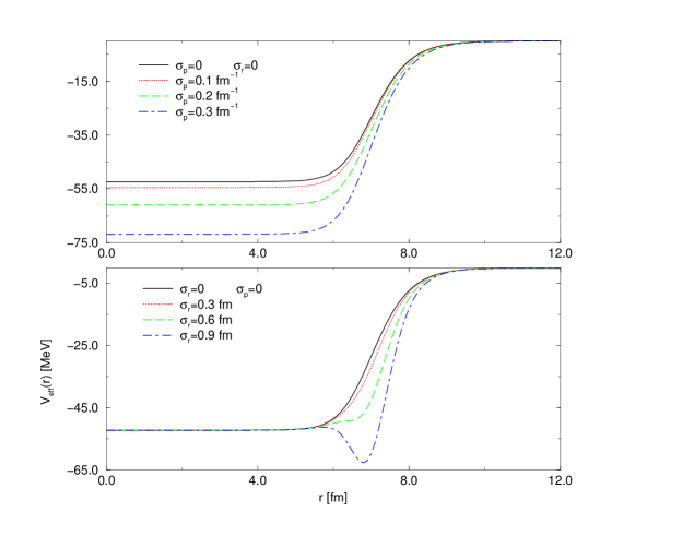
FIG. 1.: The influence of different coarse graining parameters on the selfconsistent potential. Above the space coarse graining is zero and below the momentum coarse graining is set to zero. While the momentum coarse graining leads to an increase of the selfconsistent potential the spatial coarse graining enhances the gradient and produces a skin.

A Selfconsistency

Now we return to the question of selfconsistency. We have so far assumed silently that (4) or (17) are completed by a selfconsistent potential $V(r)$. Without coarse graining this would be accomplished by solving the Thomas–Fermi–like equation (4) with $f\propto\exp{-\beta(p^{2}/2m+V(r))}$

$$V(r)={N\over g}{\int dr^{\prime}V_{0}(r-r^{\prime}){\rm e}^{-\beta V(r^{\prime})}\over\int dr^{\prime}{\rm e}^{-\beta V(r^{\prime})}}$$ (105)

and analogously for the degenerate case. For the coarse grained case we see now from (78) and (100) that the potential in the distribution function $f$ has to be replaced by

$$V_{\rm eff}(r)=V(r)+\beta\left[{\sigma_{p}^{2}\over m}V(r)-{\sigma_{r}^{2}\over 2}(\partial_{r}V(r))^{2}\right].$$ (106)

Therefore one can solve the Thomas Fermi like equation (105) as before but replace afterwards $V\rightarrow V_{\rm eff}$. In the following let us assume we have solved the Thomas–Fermi equation (105) and we will discuss now the influence of coarse graining.

We see that the coarse graining in momentum space increases the potential (106) globally. In contrast, the coarse graining in space causes a widening of the potential. This is demonstrated in figure 1, where we assume a Wood–Saxon potential for $V(r)$ in ${}^{208}Pb$ and plotted the change of the potential for different parameters of coarse graining at a temperature of $10$ MeV. While the momentum coarse graining leads to an overall increase, the spatial graining sharpens the gradient in the potential and causes the appearance of a skin.

One can consider this as a modification of the Thomas- Fermi equation by the finite width of phase space graining. The coarse graining obviously produces higher binding properties and larger rms- radii. The appearance of a skin is important to note as a relict of the testparticle width.

B Consequences on collective modes

As a practical application we show now that the coarse graining which is numerically unavoidable leads to false predictions concerning the energy and the width of giant resonances. For illustrative purpose we restrict to the low temperature $T=0$ case. The collective mode is given by the complex zeros $\omega=E-i\Gamma$ of the denominator of (86). This solution provides us with the centroid energy $E$ and damping $\Gamma$ of the collective mode. We find for $T=0$ the dispersion relation

$$1-V\Pi(q,\omega)\equiv 1+F_{0}(1+{\sigma_{p}^{2}\over 2p_{f}^{2}}{\partial^{2}\over\partial u^{2}})$$ (107)

$$\times\left[-1+{u\over 2}{\rm ln}\left({1+u\over 1-u}\right)-i{\pi\over 2}u\Theta(1-u)\right]=0$$ (108)

where we have introduced $u=m\omega/p_{f}/k$, the Landau parameter $F_{0}={2V^{\prime}(n_{0})mp_{f}\over\pi^{2}\hbar^{3}}$ and the Fermi momentum $p_{f}$.

FIG. 2.: The centroid energy and width of collective motion versus the pseudoparticle width in the low-temperature linear regime (108). The values are scaled to the free one $\sigma_{p}=0$.

In Figure 2 we give the ratio of the centroid energy and damping to the corresponding un-coarse grained ones for typical nuclear situation. We see that with increasing width of coarse graining the centroid energy decreases and the width increases. This is understandable because due to coarse graining we lower the particle- hole threshold resulting into lower centroid energy and an artificial damping at the same time. Since coarse graining is unavoidable in numerical implementations the extraction of damping width of giant resonances should be critically revised with respect to the used pseudoparticle width.

In contrast to the coarse graining in momentum space, we find a different behavior in spatial domain. In figure 3 we plot a realistic numerical solution of the full Vlasov equation describing monopole resonances in ${}^{40}Ca$. Here the spatial width of the test particles has been varied. We see that the centroid energy is increasing with increasing testparticle width. This behavior can be understood from figure 1. The spatial coarse graining enlarges the gradient of the potential and therefore increases the restoring force. This translates into a higher incompressibility and a higher collective energy.

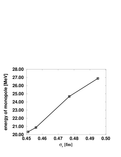
FIG. 3.: The centroid energy of monopole resonance in ${}^{40}Ca$ versus spatial testparticle width within a Vlasov simulation. The centroid energy is increasing with increasing width.

A more complete discussion of the solution of Vlasov equation and also application to giant resonances far from the stability line can be found in [45].

VI Summary

The dissipative features of coarse grained Vlasov equations are investigated. This procedure occurs due to numerical simulation techniques. We have calculated explicitly the entropy production, which is due to nonlinear mode coupling but not due to dissipation. We find that a sum of modified Boltzmann distributions is approached by the coarse graining. Examples are shown where no stationary condition is approached at all since the solution oscillates and examples are given where a stationary solution can be reached. The different behavior is completely determined by the initial distribution and the used potential. The stability analysis leads to a criterion for the initial distribution dependent on the width of test particles, which can only lead to stationary solutions.

We have demonstrated by a special model that the two steps, coarse graining and dynamical evolution of the distribution function, are only interchangeable if the initial distribution is also coarse grained. It is argued that this property does not hold in general due to the feedback of the selfconsistent potential. Because the coarse graining is unavoidable in numerically implementations, the Vlasov codes should be critically revised with respect to the question if they start really from a coarse grained initial distribution.

Thermodynamical consequences are discussed. A correlated part to any thermodynamical observable is calculated explicitly. It is given in terms of the space and momentum width. We find that the selfconsistently determined nuclear potential is overestimated by testparticle simulations with finite width of the test particles. This should have implementations on Thomas- Fermi calculations where an overbinding is found.

The linear response function is calculated for homogeneous systems and the spectra of density fluctuation is presented. It is found that the RPA polarization function becomes modified due to the finite momentum width of testparticles. These modifications can be understood as an internal structure the particles bear. This structure function is formally compared with vertex corrections to the RPA. It is pointed out that the higher order vertex corrections beyond RPA can be casted into similar structure functions. Therefore we suggest a method of simulating higher order correlations in one-body treatments by choosing an appropriate momentum width of testparticles.

As a practical consequence the collective mode is analyzed. We find that the coarse graining enhances the damping width and lowers the centroid energy of collective modes, e.g. giant resonances. The dependence on the coarse graining width is given quantitatively and corresponding simulations should be revised.

VII Acknowledgments

The authors are especially indebted to P.G. Reinhard for many discussions and critical comments. The model IIIA has been contributed by him. J. Dorignac is thanked for critical reading and helpful comments. The friendly and hospitable atmosphere of LPC in Caen is gratefully acknowledged.

A Refined testparticle picture

We want to consider now the question how the dynamics is influenced by coarse graining. While the original Vlasov equation (2) is represented by the Hamilton dynamics of testparticles via (3), we like to know how the equation of motions are changed by coarse graining. Therefore we obtain with (11) the coarse grained kinetic energy $K$ and the potential energy $W$ as

$$K(t) = \int{dpdr\over(2\pi\hbar)^{3}}{p^{2}\over 2m}f_{\delta}(p,r,t)$$ (A1)

$$\equiv \int{dpdr\over(2\pi\hbar)^{3}}{p^{2}+\sigma_{p}^{2}\over 2m}f(p,r,t)$$ (A2)

$$W(t) = \frac{1}{2}\int{dpdr\over(2\pi\hbar)^{3}}V_{\delta}(r,t)f_{\delta}(p,r,t)$$ (A3)

$$\equiv \frac{1}{2}\int{dpdr\over(2\pi\hbar)^{3}}V(r,t)\rm{exp}(\sigma_{r}^{2}{\stackrel{{\scriptstyle\leftarrow}}{{\partial}}_{r}}{\stackrel{{\scriptstyle\rightarrow}}{{\partial}}_{r}})f(p,r,t).$$ (A4)

We see that the coarse graining in momentum space leads to an additional apparent temperature $\sigma_{p}^{2}=mT$, while the coarse graining in space modifies the potential and therefore the dynamics.

With the help of (3) and (7) we find from the variation of the action $\int dt(K(t)-W(t))$ just the Hamilton equations

$${\partial\over\partial\,t}R_{i}(t) = {P_{i}(t)\over m}$$ (A5)

$${\partial\over\partial\,t}P_{i}(t) = -{\partial\over\partial\,R_{i}}V_{\delta}(R_{i},t)$$ (A6)

irrespective which form we use of (A4). This is clear because the underlying dynamics is entirely covered by the Hamiltonian dynamics. Therefore even the center of mass movement of the Gauß packets $R_{i},P_{i}$ follows the Hamilton dynamics.

We may now turn the question around and define a new quasi(test)- particle picture. We seek the equation of motion for new testparticles $(\tilde{P}_{i},\tilde{R}_{i})$ which should now represent the coarse grained distribution (7)

$$f(prt) = \{f_{\delta}\}_{g}$$ (A7)

$$= \sum\limits_{i=1}^{\infty}g_{r}(r-R_{i}(t))g_{p}(p-P_{i}(t))$$ (A8)

$$\equiv \sum\limits_{i=1}^{\infty}\delta(r-\tilde{R}_{i}(t))\delta(p-\tilde{P}_{i}(t)).$$ (A9)

The last step is just the definition of the new test particles which obey the equation of motion derived from (A4)

$${\partial\over\partial\,t}\tilde{R}_{i}(t) = {\tilde{P}_{i}(t)\over m}$$ (A10)

$${\partial\over\partial\,t}\tilde{P}_{i}(t) = -{\partial\over\partial\,\tilde{R}_{i}}{\rm e}^{-\sigma_{r}^{2}\partial_{\tilde{R}_{i}}^{2}}V(\tilde{R}_{i},t)$$ (A11)

with $V$ the coarse grained mean field (17). We observe that the coarse grained distribution $f$ can be represented by a set of quasi(test)- particles which obey Hamilton equations with a modified effective potential

$$V_{\rm eff}(r,t) = {\rm e}^{-\sigma_{r}^{2}\partial_{r}^{2}}V(r,t)$$ (A12)

$$\approx V(r,t)-\sigma_{r}^{2}\partial_{r}^{2}V(r,t).$$ (A13)

We see that the relation between the coarse grained mean field potential (17) and the effective one can be written as a double folding

$$V(r,t) = {\rm e}^{\sigma_{r}^{2}\partial_{r}^{2}}V_{\rm eff}(r,t)\equiv\{\{V_{\rm eff}(r,t)\}_{g_{r}}\}_{g_{r}}$$ (A14)

or

$$V_{\delta}(r,t) = \{V_{\rm eff}(r,t)\}_{g_{r}}$$ (A15)

where we have used the relation $\{f(r)\}_{g_{r}}=\exp{({\sigma^{2}\over 2}\partial_{r}^{2})}f(r)$, see [46]. Please observe that the here presented relation is just the inverse relation given in [38, 39, 40]. The difference comes from the inverse picture used here. The authors of [38, 39, 40] investigated how the dynamical equation change if in the action the distribution functions are replaced by their coarse grained ones. We present here the opposite view that the action is unchanged but is rewritten according to coarse graining, leading to modified explicit kinetic and potential energy (A4). This still leads to unmodified equation of motions for the center of mass coordinates of the Gauß packets as outlined above. When we now represent the coarse grained distribution by a new set of sharp testparticles, the dynamics becomes modified and an effective potential appears which is the inverse folded mean field potential (A15).

We conclude that we can map the coarse grained Vlasov equation to the original Vlasov equation if testparticles are introduced which obey a modified dynamical equation with the new inverse folded mean field potential. Within the text we have followed the other route to describe the influence on the dynamics in the old picture to make the effects more transparent.

B Coarse graining of selfconsistent model

Here we give the explicit calculations of chapter III B.

a First solving than coarse graining

We like to choose as an initial condition a Gaussian distribution, which represents an equilibrium distribution

$$f_{0}({\bf x}) = \left(2\pi\right)^{-3}\sqrt{\mbox{Det}\{{\hat{\bf\Lambda}}\}}e^{-\frac{1}{2}{\bf x}^{T}\hat{{\bf\Lambda}}{\bf x}}$$ (B1)

with

$${\hat{\bf\Lambda}}=\left(\begin{array}[]{cc}\mu&0\\ 0&\lambda\end{array}\right)\quad.$$ (B2)

Then the solution (60) of the selfconsistent Vlasov equation reads

$$f_{\delta}({\bf x},t)=\left(2\pi\right)^{-3}\sqrt{\mbox{Det}\{\hat{{\bf\Lambda}}\}}e^{-\frac{1}{2}(\hat{\bf A}{\bf x}+{\bf C})^{T}{\hat{\bf\Lambda}}(\hat{\bf A}{\bf x}+{\bf C})}$$ (B3)

$$=\left(2\pi\right)^{-3}\sqrt{\mbox{Det}\{\hat{{\bf\Lambda}}\}}e^{-\frac{1}{2}({\bf x}^{T}+{\bf C}^{T}(\hat{\bf A}^{T})^{-1})\hat{\bf A}^{T}{\hat{\bf\Lambda}}\hat{\bf A}({\bf x}+\hat{\bf A}^{-1}{\bf C})}.$$ (B4)

We can now coarse grain the distribution with (36) to obtain the result

$$f({\bf x},t) = {\left(2\pi\right)^{-3}e^{-\frac{1}{2}(\hat{\bf A}{\bf x}+{\bf C})^{T}(\hat{\bf\Lambda}^{-1}+\tilde{{\bf\Sigma}}^{-1})^{-1}(\hat{\bf A}{\bf x}+{\bf C})}\over\sqrt{\mbox{Det}\{(\hat{\bf A}^{T}{\hat{\bf\Lambda}}\hat{\bf A})^{-1}+\hat{{\bf\Sigma}}\}}}$$ (B6)

where

$$\tilde{\bf\Sigma}=\hat{\bf A}\hat{\bf\Sigma}\hat{\bf A}^{T}.$$ (B8)

We see that the coarse grained solution (LABEL:sola) can be represented at any time by the coarse grained initial distribution

$$f({\bf x},t) = \{f_{\delta}({\bf x},t)\star{\cal G}({\bf x})\}({\bf y})$$ (B9)

$$= \{f_{0}(\hat{\bf A}{\bf x}+{\bf C})\star{\cal G}({\bf x},t)\}({\bf y})$$ (B10)

$$= \{f_{0}({\bf x})\star\tilde{\cal G}({\bf x},t)\}(\hat{\bf A}{\bf y}+{\bf C})$$ (B11)

if we use the coarse graining (36) but with the ( now time dependent) width (B8). It is immediately obvious that the last identity in (B11) is only valid if we use Gaussian initial distributions. Any other distributions will not allow this rearrangement. Consequently the folding and the dynamics are not interchangeable in general.

The entropy is calculated from (LABEL:sola)

$$S=3\log{(2\pi e)}+\frac{1}{2}\log{{\rm Det}((\hat{\bf A}^{T}{\hat{\bf\Lambda}}\hat{\bf A})^{-1}+\hat{{\bf\Sigma}})}\quad$$ (B12)

with the explicit expression (70).

b First coarse graining than solving

Equation (20) is transformed into a partial differential equation of first order by Fourier transform ${\bf x}=(r,p)\rightarrow{\bf q}=(q,x)$. The solution can be obtained for the Fourier transformed distribution $\tilde{f}$

$$\tilde{f}({\bf q},t)=\tilde{f}_{0}((A^{-1})^{T}{\bf q})\exp(\frac{1}{2}{\bf q}^{T}\hat{\bf B}{\bf q}+{\bf D}{\bf q})$$ (B13)

with the matrix $\hat{\bf A}$ as defined in (59) and

$${\bf D} = iva\int\limits^{t}dt^{\prime}Q(t^{\prime})\left(\matrix{{\sin(\omega(t-t^{\prime}))\over m\omega}\cr\cos(\omega(t-t^{\prime}))}\right)$$ (B14)

$$\hat{\bf B} = \frac{1}{2}({\sigma_{p}^{2}\over m\omega}-\sigma_{r}^{2}m\omega)\left(\matrix{{1-\cos(2\omega t)\over m\omega}&\sin(2\omega t)\cr\sin(2\omega t)&m\omega(1-\cos(2\omega t))}\right).$$ (B16)

The selfconsistency requirement (49) leads to the same solution as (62). This shows that the coarse graining does not affect the nonlinear feedback of the selfconsistent potential within this model. In other more nontrivial models this needs not to be the case.

If we now use as initial distribution once more a Gaussian (B1) which reads in Fourier transform

$$\tilde{f}_{0}({\bf q})=\exp(-\frac{1}{2}{\bf q}^{T}\hat{\bf\Lambda}^{-1}{\bf q})$$ (B18)

we obtain the time dependent distribution after inverse Fourier transform

$$f({\bf x})={(2\pi)^{-3}\over\sqrt{{\rm Det}\{\hat{M}\}}}\exp{\left[\!-\!\frac{1}{2}({\bf x}\!-\!i{\bf D})^{T}\hat{\bf M}^{-1}({\bf x}\!-\!i{\bf D})\right]}$$ (B19)

with

$$\hat{\bf M}=(\hat{\bf A}^{T}\hat{\bf\Lambda}\hat{\bf A})^{-1}-\hat{\bf B}.$$ (B20)

REFERENCES

- [1] G. F. Burgio, P. Chomaz, and J. Randrup, Phys. Rev. Lett. 69, 885 (1992).
- [2] G. Peilert et al., Phys. Rev. C 39, 1402 (1989).
- [3] B. ter Haar and R. Malfliet, Phys. Lett. B 172, 10 (1986).
- [4] G. F. Bertsch, H. Kruse, and S. DasGupta, Phys. Rev. C 29, 673 (1984), errata: 33 (1986) 1107.
- [5] G. F. Bertsch and S. D. Gupta, Phys. Rep. 160, 189 (1988).
- [6] P. Danielewicz, Ann. Phys. (NY) 152, 239 (1984).
- [7] C. Gregoire et al., Nucl. Phys. A 465, 317 (1987).
- [8] W. Bauer, Nucl. Phys. A 538, 83 (1992).
- [9] J. Aichelin and G. Bertsch, Phys. Rev. C 31, 1730 (1985).
- [10] D. Klakow, G. Welke, and W. Bauer, Phys. Rev C 48, 1982 (1993).
- [11] K. Morawetz et al., Phys. Rev. Lett. 82, 3767 (1999).
- [12] H. S. Köhler and B. S. Nilsson, Nucl. Phys. A 417, 541 (1984).
- [13] P. Danielewics, Phys. Lett. B 146, 168 (1984).
- [14] H. S. Köhler, Nucl. Phys. A 440, 165 (1984).
- [15] M. M. Abu-Samreh and H. S. Köhler, Nucl. Phys. A 552, 101 (1993).
- [16] H. S. Köhler and W. Bauer, Phys. Rev. C 40, 1711 (1989).
- [17] L. W. Nordheim, Proc. Roy. Soc. (A) 119, 689 (1928).
- [18] E. A. Uehling and G. E. Uhlenbeck, Phys. Rev. 43, 552 (1933).
- [19] C. Gale, G. Bertsch, and S. DasGupta, Phys. Rev. C 35, 1666 (1987).
- [20] H. Kruse, B. V. Jacak, and H. Stocker, Phys. Rev. Lett. 54, 289 (1985).
- [21] H. Stöcker and W. Greiner, Phys. Rep. 137, 277 (1986).
- [22] J. Cugnon, A. Lejeune, and P. Grangé, Phys. Rev. C 35, 861 (1987).
- [23] V. Špička, P. Lipavský, and K. Morawetz, Phys. Lett. A 240, 160 (1998).
- [24] K. Morawetz, P. Lipavský, V. Špička, and N. H. Kwong, Phys. Rev. C 59, 3052 (1999).
- [25] K. Morawetz et al., Phys. Rev. C 63, 034619 (2001).
- [26] P. Bonche, S. Koonin, and J. Negele, Phys. Rev. C 13, 1226 (1976).
- [27] C. Y. Wong, Phys. Rev. C 25, 1460 (1982).
- [28] A. Bonasera, G. F. Bertsch, and E. N. El-Sayed, Phys. Lett. B 141, 9 (1984).
- [29] M. Groß and C. Guet, Phys. Rev. A 54, R2547 (1996).
- [30] L. Plagne and C. Guet, Phys. Rev. A 59, 4461 (1999).
- [31] F. Calvayrac, P. G. Reinhard, E. Suraud, and C. A. Ullrich, Phys. Rep 337, 493 (2000).
- [32] C. Jarzynski and G. F. Bertsch, Phys. Rev. C 53, 1028 (1996).
- [33] Y. L. Klimontovich, Kinetic theory of nonideal gases and nonideal plasmas (Academic Press, New York, 1975).
- [34] P. Lipavský, K. Morawetz, and V. Špička, Kinetic equation for strongly interacting dense Fermi systems (Annales de Physique, Paris, 2001), No. 26, 1, K. Morawetz, Habilitation University Rostock 1998.
- [35] J. W. Gibbs, in Elementare Grundlagen der statistischen Mechanik (J. A. Barth, Leipzig, 1905).
- [36] P. Ehrenfest and T. Ehrenfest, Enzyklopädie der Mathematischen Naturwissenschaften (1907-1914), No. 4, p. Art. 32.
- [37] D. N. Zubarev, Statistische Thermodynamik des Nichtgleichgewichts (Akademie Verlag, Berlin, 1976).
- [38] P. G. Reinhard and E. Suraud, Ann. of Phys. 239, 193 (1995).
- [39] P. G. Reinhard and E. Suraud, Ann. of Phys. 239, 216 (1995).
- [40] P. L’Eplattenier, E. Suraud, and P. G. Reinhard, Ann. of Phys. 244, 426 (1995).
- [41] K. Takahashi, Prog. of Theor. Phys. Suppl. 98, 109 (1989).
- [42] K. Morawetz, Phys. Rev. C 55, R 1015 (1997).
- [43] K. Morawetz et al., Phys. Rev. C. 60, 54601 (1999).
- [44] K. Morawetz, Phys. Rev. E. 61, 2555 (2000).
- [45] K. Morawetz, U. Fuhrmann, and R. Walke, in Isospin Effects in Nuclei, edited by B. A. Lie and U. Schroeder (World Scientific, Singapore, 2000), correct version: nucl-th/0001032.
- [46] R. F. O’Connell, L. Wang, and H. A. Williams, Phys. Rev. A 30, 2187 (1984).