Critical analysis of quark-meson coupling models for nuclear matter and finite nuclei

Abstract

Three versions of the quark-meson coupling (QMC) model are applied to describe properties of nuclear matter and finite nuclei. The models differ in the treatment of the bag constant and in terms of nonlinear scalar self-interactions. In two versions of the model the bag constant is held fixed at its free space value whereas in the third model it depends on the density of the nuclear environment. As a consequence opposite predictions for the medium modifications of the internal nucleon structure arise. After calibrating the model parameters at equilibrium nuclear matter density, binding energies, charge radii, single-particle spectra and density distributions of spherical nuclei are analyzed and compared with QHD calculations. For the models which predict a decreasing size of the nucleon in the nuclear environment, unrealistic features of the nuclear shapes arise.

I Introduction

Although quantum chromodynamics is believed to be the fundamental theory of strong interactions, low- and medium-energy nuclear phenomenology is successfully described in terms of hadronic degrees of freedom. Theoretical challenges arise in phenomena which reveal the quark structure of hadrons. Building models which connect observed nuclear phenomena and the underlying physics of strong interactions has become one of the fundamental goals in nuclear physics. Such models are necessarily crude and contain a variety of unknown parameters since the study of the nuclear many-body problem on the fundamental level is intractable. However, it is important that the new models respect established results which are successfully described in the hadronic framework.

The quark-meson coupling (QMC) model proposed by Guichon [1], provides a simple framework to incorporate quark degrees of freedom in the study of nuclear many-body systems. In the QMC model nucleons arise as non-overlapping MIT bags interacting through meson mean fields. The model has been applied to a variety of problems in nuclear physics. It was shown that it describes the saturation properties of nuclear matter [2, 3, 4, 5, 6, 7], and that it gives a fair description of the bulk properties of finite nuclei [8, 9, 10, 11, 12, 13]. The model was extended to include hyperons [14] and applied to studies of hyper-nuclei [15, 16].

Although it provides a simple and intuitive framework to describe the basic features of nuclear systems in terms of quark degrees of freedom, the QMC model has a serious shortcoming. It predicts much smaller scalar and vector potentials than obtained in successful hadronic models [3, 5, 6]. As a consequence the nucleon mass is too high and the spin-orbit force is too weak to explain spin-orbit splittings in finite nuclei [9, 10, 11].

The QMC model can be significantly improved by introducing the concept of a density dependent bag constant [5, 6]. The modified quark-meson coupling (MQMC) produces large scalar and vector potentials under the condition that the value of the bag constant in the nuclear environment significantly drops below its free-space value.

In the present work we study three different versions of the QMC model. The first model is the original QMC model which we denote by QMCI. The second model denoted by QMCII is an extension which includes cubic and quartic self interactions for the scalar meson. As our third model we adopt model ${\rm MQMC}_{\rm A}$ from Ref. [7], in which the bag constant is a function of the scalar field.

The original idea of the QMC model was to calibrate the model in free space such that the nucleon mass is reproduced and then to extrapolate to many-nucleon systems. However, it is not possible to account for all the necessary degrees of freedom. Most importantly, the scalar field which describes the mid-range part of the nucleon-nucleon interaction cannot be described in the framework of the simple bag model, but it must be included. The additional cubic and quartic scalar self-interactions of the QMCII model were introduced in Refs. [11] to model the density dependence of the scalar mass. The corresponding couplings cannot be determined on a fundamental level [11]. In our approach we choose these parameters to reproduce the properties of nuclear matter near equilibrium that are known to be characteristic of the observed bulk and single-particle properties of nuclei. This procedure guarantees the reproduction of large scalar and vector potentials.

In the MQMC model new parameters arise from the unknown density dependence of the bag constant. A refined MQMC model can be accurately calibrated to produce the empirical saturation properties of nuclear matter [7] and it provides a good description of the bulk properties of finite nuclei [13]. Most importantly, the model can be calibrated to reproduce small values for the effective nucleon mass which leads to a realistic description of spin-orbit splittings [13].

One of the basic motivations of applying quark models to nuclear systems is the hope to describe medium modifications of the internal quark-substructure of the nucleon. An important phenomenological quantity is the nucleon size which is represented in the framework of the QMC model by the bag radius [17]. Due to the increase of the bag constant the MQMC model predicts significantly swollen nucleons in the nuclear environment [5, 6, 7]. In contrast, for the QMCI and II model the bag radius decreases with increasing density[3, 8, 9, 11]

Our main goal is to study properties of nuclear matter and finite nuclei. We investigate whether the different versions of the QMC model lead to results which are consistent with established hadronic phenomenology. At present such an analysis might provide the only testing ground for the reliability of the strikingly different predictions for the changes of the internal nucleon structure.

A well established framework for relativistic hadronic models is provided by quantum hadrodynamics (QHD) [18]. Numerous calculations have established that relativistic mean-field models based on QHD lead to a realistic description of nuclear matter and of the bulk properties of finite nuclei throughout the Periodic Table [18, 19, 20, 21, 22, 23, 24, 25]. A very compelling feature of QHD has been the reproduction of spin-orbit splittings in finite nuclei. For comparison we employ a QHD model that includes quartic and cubic scalar self-interactions. We calibrate the model parameters so that QMCII, MQMC and QHD lead to the same nuclear matter properties at equilibrium. The QMCI does not provide a sufficient number of parameters to fit all the desired nuclear matter properties. Particularly, a rather high value for the effective nucleon mass at equilibrium is a prediction in this model [3].

In our previous work [7, 13] we demonstrated that the QMC models are equivalent to a QHD type mean field model with a general nonlinear scalar potential and a coupling to the gradients of the scalar field. One of the key observations in the success of hadronic models is that nonlinear scalar self-interactions, i.e. a nonlinear potential, must be included [19, 20, 21, 22, 23, 24, 25, 26, 27]. This potential is constrained by nuclear observables and we check if the QMC models predict the typical size and form of the potential.

In nuclear matter we find that the models which can be accurately calibrated, namely QMCII, MQMC and QHD, lead to essentially identical results. The MQMC and QMCII models reproduce large scalar and vector potentials and the typical size of the nonlinear potential. In contrast, the QMCI model leads to rather small scalar and vector mean fields. At the equilibrium point the nonlinear potential has only half the size of the value predicted by the other models.

The results for the binding energies and spin-orbit splittings are similar. The QMCII, MQMC and QHD model, which reproduce the empirical properties of nuclear matter, lead to a realistic description of the experimental numbers; the only exception are the light nuclei. The surface energy in the QMCII model is too small and as a consequence the light systems are systematically overbound. The QMCI model underestimates the binding energies and gives only a poor reproduction of single-particle spectra and spin-orbit splittings [8, 9, 10, 11]. The key observations is that the MQMC and QMCII model can reproduce sufficient small values for the effective mass, which is strongly correlated with the spin-orbit force in relativistic mean-field models.

The main difference between the models arises from the nonlinear coupling to the gradient of the scalar field. The coupling has no effect in nuclear matter and its size is a prediction of the underlying bag model. It mainly effects the nuclear shapes leading to more diffuse surfaces in the QMC models. At normal nuclear matter density the gradient coupling in the QMCII model is 6-7 times bigger than in the MQMC model. From the point of view of an effective field theory a gradient coupling arises naturally as a subset of possible nonlinear meson-meson interactions [25]. However, rather than attempting to compete with these more sophisticated versions of QHD, it is our goal to analyze if an approach which is based on a simple quark model can reproduce well established results of nuclear phenomenology. For comparison we employ a more conventional version of QHD which does not include the gradient coupling. We compensate the effect on the nuclear shapes by adjusting the scalar mass to reproduce the experimental value of the charge radius in ${}^{40}{\rm Ca}$. Although after the adjustment all the models predict nearly identical rms charge radii we find sizable differences in the predicted density profiles. The QMCI and QMCII model lead to very compact nuclei with small central densities and steep surface areas. This effect is more pronounced for the light nuclei.

The outline of this paper is as follows: In Sec. II, we review the formalism for finite nuclei and nuclear matter. Section III contains a short summary of the QMC model and the relations which determine the properties of the nucleon. We also briefly discuss the calibration procedure. In Sec. IV, we analyze nuclear matter. We concentrate on the predictions for the nonlinear potential. In Sec. V, we apply the models to finite nuclei. Sec. VI contains a short summary and our conclusions.

II The Quark-Meson Coupling Model for Nuclear Systems

To study the properties of finite nuclei and nuclear matter we use a relativistic mean-field model containing nucleons, neutral scalar ($\phi$) and vector fields ($V_{\mu}$) and the isovector $\rho$ meson field ($\mathbf{b}_{\mu}$). For a realistic description of finite nuclei, the electromagnetic field ($A_{\mu}$) must also be included. We assume the nucleons obey the Dirac equation

$$\left(i\not{\!\partial}-\not{\!\mathcal{V}}-{1\over 2}\mbox{\boldmath$\tau\cdot$}\not{\!\mbox{\boldmath$\mathcal{B}$}}-{1\over 2}(1+\tau_{3})\not{\!\!\mathcal{A}}-M^{*}\right)\psi_{\scriptscriptstyle N}(x)=0\ .$$ (1)

The potentials ($\mathcal{V}^{\nu},\mbox{\boldmath$\mathcal{B}$}^{\nu},\mathcal{A}^{\nu}$) and the effective mass $M^{*}$ are functionals of the meson mean fields, their form depends on the underlying quark model.

In the QMC model the quarks are described by the Dirac equation

$$\left(i\not{\!\partial}-g_{\rm v}^{q}\not{\!V}-{1\over 2}g_{\rho}^{q}\mbox{\boldmath$\tau\cdot\not{b}$}-(1+3\tau_{3}){e\over 6}\not{\!\!A}-[m_{q}-g_{\rm s}^{q}\phi]\right)\psi_{q}(x)=0\ ,$$ (2)

where $m_{q}$ is the current quark mass. The quark wave function is subject to the bag model boundary conditions at the surface of the bag. Because quarks and nucleons interact with the meson mean fields, Eqs. (1) and (2) define a self-consistent scheme for the description of the nuclear system. In infinite nuclear matter (${\mathcal{A}}^{\nu}=0$) the meson mean fields are constant and the potentials are given by [3, 8, 9]

$${\mathcal{V}}^{\nu} = 3g_{\rm v}^{q}\,V^{\nu}\equiv g_{\rm v}\,V^{\nu}\ ,$$ (3)

$$\mbox{\boldmath$\mathcal{B}$}^{\nu} = g_{\rho}^{q}\,{\mathbf{b}}^{\nu}\equiv g_{\rho}\,{\mathbf{b}}^{\nu}\ .$$ (4)

The effective mass is an ordinary function of the scalar field, i.e.

$$M^{*}=M^{*}(\phi)\ .$$ (5)

For a finite system the solution of Eq. (1) and Eq. (2) is rather complicated due to the variation of the meson mean fields over the bag volume. In consequence, the quark wave function and the ground state of a bound nucleon are no longer spherically symmetric [10]. To make a numerical solution feasible it is necessary to calculate the quark properties by using some suitably averaged form for the meson mean fields. Here we follow the prescription of [8, 9, 11] and replace the meson mean fields on the quark level by their value at the center of the nucleon bag, i.e. we neglect the spatial variation of the mean fields over the bag volume. In this local density approximation the potentials in Eq. (1) are simply obtained by the corresponding nuclear matter relations given by Eqs. (4) and Eq. (5). The corresponding relation for the electromagnetic field is

$${\mathcal{A}}^{\nu} = e\,A^{\nu}\ .$$ (6)

If we restrict considerations to spherically symmetric nuclei only the $V_{0}$ component of the neutral vector field and the neutral $\rho$ meson field (denoted by $b_{0}$) contribute. The ground state energy of a nucleus can be written as

$$E_{\scriptscriptstyle N} = \sum_{i=occ.}E_{i}+\int\,dV\Biggl{(}[{1\over 2}(\nabla\phi)^{2}+U_{\rm s}(\phi)]-{1\over 2}[(\nabla V_{0})^{2}+m_{\rm v}^{2}V_{0}^{2}]$$ (8)

$$\hbox{}-{1\over 2}[(\nabla b_{0})^{2}+m_{\rho}^{2}b_{0}^{2}]-{1\over 2}(\nabla A_{0})^{2}\Biggr{)}\ ,$$

where $E_{i}$ are the eigenvalues of the Dirac equation Eq. (1).

To analyze a general class of models, we introduce a nonlinear scalar potential of the form

$$U_{\rm s}(\phi)={1\over 2}m^{2}_{\rm s}\phi^{2}+{1\over 3!}\kappa\phi^{3}+{1\over 4!}\lambda\phi^{4}\ .$$ (9)

The actual mean field configuration is obtained by extremization of the energy. This leads to the set of self-consistency equations

$$\Delta\phi-{\partial U_{\rm s}\over\partial\phi} = {\partial\over\partial\phi}M^{*}(\phi)\rho_{\rm s}\ ,$$ (10)

$$\bigl{(}\Delta-m_{\rm v}^{2}\bigr{)}V_{0} = -g_{\rm v}\rho\ ,$$ (11)

$$\bigl{(}\Delta-m_{\rho}^{2}\bigr{)}b_{0} = -g_{\rho}{1\over 2}\rho_{3}\ ,$$ (12)

$$\Delta A_{0} = -e\rho_{p}\ .$$ (13)

The densities on the right-hand side are the nuclear densities calculated with the wave functions in Eq. (1):

$$\rho_{\rm s} = \sum_{i=occ.}\bar{\psi}_{\scriptscriptstyle N}^{i}\psi_{\scriptscriptstyle N}^{i}\ ,$$ (14)

$$\rho = \sum_{i=occ.}\bar{\psi}_{\scriptscriptstyle N}^{i}\gamma^{0}\psi_{\scriptscriptstyle N}^{i}\ ,$$ (15)

$$\rho_{3} = \sum_{i=occ.}\bar{\psi}_{\scriptscriptstyle N}^{i}\tau_{3}\gamma^{0}\psi_{\scriptscriptstyle N}^{i}\ ,$$ (16)

$$\rho_{p} = {1\over 2}\sum_{i=occ.}\bar{\psi}_{\scriptscriptstyle N}^{i}(1+\tau_{3})\gamma^{0}\psi_{\scriptscriptstyle N}^{i}\ .$$ (17)

In the limit of infinite symmetric nuclear matter Eqs. (8) simplifies to

$${E_{\scriptscriptstyle N}\over V}={2\over\pi^{2}}\int_{0}^{k_{\rm F}}dk\,k^{2}(k^{2}+M^{*}{}^{2})^{1/2}+g_{\rm v}V_{0}\rho-{1\over 2}m_{\rm v}^{2}V_{0}^{2}+U_{\rm s}(\phi)\ .$$ (18)

For the time-like component of the vector field Eq. (11) reduces to

$$g_{\rm v}V_{0}={g_{\rm v}^{2}\over m_{\rm v}^{2}}\rho\ ,$$ (19)

whereas the scalar field is determined by the equivalent of Eq. (10):

$${\partial U_{\rm s}\over\partial\phi}=-{\partial M^{*}\over\partial\phi}\ {2M^{*}\over\pi^{2}}\int_{0}^{k_{\rm F}}dk\,{k^{2}\over(k^{2}+M^{*}{}^{2})^{1/2}}\ .$$ (20)

In symmetric matter the Fermi momentum of the nucleons is related to the conserved baryon density by

$$\rho={2\over 3\pi^{2}}k_{\rm F}^{3}\ .$$ (21)

The details of the underlying quark substructure are entirely contained in the expression for the effective mass $M^{*}(\phi)$. In the next section we will discuss the functional form of the effective mass in the framework of the QMC model.

III The Quark-Meson Coupling Model

In this section, we briefly summarize the relations which determine the nuclear equation of state in the quark-meson coupling model. For further details we refer the reader to Refs. [3, 5, 6].

In the QMC model the nucleon in the nuclear medium is described as a static, spherical MIT bag in which quarks couple to meson mean fields.

The energy of a bag consisting of three quarks in the ground state can be expressed as

$$E_{bag}=3{\Omega_{q}\over R}-{Z\over R}+{4\over 3}\pi R^{3}B\ .$$ (22)

where the parameter $Z$ accounts for the zero point motion and $B$ is the bag constant. The coupling of the quarks to the scalar field is inherent in the quantities $\Omega_{q}$ and $x$ which are given by

$$\Omega_{q} = \sqrt{x^{2}+(Rm_{q}^{*})^{2}}$$ (23)

$$j_{0}(x) = \left({\Omega_{q}-Rm_{q}^{*}\over\Omega_{q}+Rm_{q}^{*}}\right)^{1/2}j_{1}(x)\ ,$$ (24)

and where $m_{q}^{*}=m_{q}^{0}-g_{\phi}^{q}\phi$ denotes the effective quark mass and $m_{q}^{0}$ is the current quark mass. In the following we choose $m_{q}^{0}=5$ MeV.

To remove the spurious center-of-mass motion in the bag we follow Ref. [8] and adjust the parameter $Z$ in Eq. (22) to reproduce the experimental value of the nucleon mass in the vacuum, i.e. we take

$$M^{*}(\phi)=E_{bag}\ .$$ (25)

For a fixed meson mean-field configuration the bag radius $R$ is determined by the equilibrium condition for the nucleon bag in the medium

$${\partial M^{*}\over\partial R}=0\ .$$ (26)

In free space $M$ can be fixed at its experimental value 939 MeV and the condition Eq. (26) to determine the parameters $B=B_{0}$ and $Z=Z_{0}$. For our choice, $R_{0}=0.8$ fm, the result for $B_{0}^{1/4}$ and $Z_{0}$ are 169.97 MeV and 3.295, respectively.

In the original version of the QMC model[1, 3] the bag parameters $B$ and $Z$ were held fixed at their free space values $B=B_{0},Z=Z_{0}$. Formally, the bag constant $B$ is associated with the QCD trace anomaly. In the nuclear environment it is expected to decrease with increasing density as argued in Ref. [28].

To account for this physics in the QMC approach Jin and Jennings [5, 6] proposed two models for the medium modification of the bag constant: a direct coupling model in which the bag constant is a function of the scalar field and a scaling model which relates the bag constant directly to the effective nucleon mass. The density dependence is then generated self-consistently in terms of these in-medium quantities. In a previous work [7] this approach was generalized and it was demonstrated that the resulting improved MQMC model can be accurately calibrated to reproduce the empirical properties of nuclear matter [7] and finite nuclei [13].

For our purpose here we adopt the model ${\rm MQMC}_{\rm A}$ of Ref. [7] in which the bag constant depends on the scalar field only

$${B\over B_{0}}=\left(1-g_{\scriptscriptstyle\rm B}{\phi\over M}F(\phi)\right)^{\eta}\quad\hbox{\rm with}\quad F(0)=1\ .$$ (27)

We model the functional form of $F$ by using a simple polynomial parametrization

$$F(\phi)=1+\alpha\phi+\beta\phi^{2}\ .$$ (28)

The functional form Eq. (28) provides sufficient flexibility and it is not necessary to include further nonlinearities in the scalar potential. We therefore analyze the MQMC model with

$$U_{\rm s}(\phi)={1\over 2}m^{2}_{\rm s}\phi^{2}\ .$$ (29)

In addition we consider the original QMC model in two versions. In the first model, which we denote QMCI, we disregard the nonlinear terms in the scalar potential and use the same form as in Eq. (29). In the second model, which we denote QMCII, we include the cubic and quartic terms as given by Eq. (9). We analyze if these additional nonlinearities lead to an improvement of the model.

We close this section with a brief description of the calibration procedure. The parameters $B_{0}$ and $Z$ are fixed to reproduce the nucleon mass in the vacuum. In nuclear matter the MQMC model contains seven free parameters. The parametrization of the bag constant contains the parameter $\eta$ and the three couplings $(g_{\scriptscriptstyle\rm B},\alpha,\beta)$; in addition values for the ratios $g_{\rm s}^{q}/m_{\rm s},g_{\rm v}/m_{\rm v},g_{\rho}/m_{\rho}$ are needed.

To determine the parameters we follow [7]. For given values of $\eta$ and $g_{\rm s}^{q}/m_{\rm s}$ we determine the values of $(g_{\scriptscriptstyle\rm B},\alpha,\beta,g_{\rm v}/m_{\rm v},g_{\rho}/m_{\rho})$ to reproduce the equilibrium properties of nuclear matter, which are taken to be: the equilibrium density and binding energy ($\rho^{\scriptscriptstyle 0}$, $-e_{\scriptscriptstyle 0}$), the nucleon effective mass at equilibrium ($M_{\scriptscriptstyle 0}^{*}$) the symmetry energy ($a_{\scriptscriptstyle 4}$) and the compression modulus ($K_{\scriptscriptstyle 0}$). The set of equilibrium properties used here are listed in the first row of Table I (denoted by input). For more details concerning the calibration procedure we refer the reader to Ref. [7].

The model QMCII contains the five parameters $g_{\rm s}^{q}/m_{\rm s},g_{\rm v}/m_{\rm v},g_{\rho}/m_{\rho},\kappa$ and $\lambda$ which are determined to reproduce the same equilibrium properties as for the MQMC model. In the model QMCI only the parameters $g_{\rm s}^{q}/m_{\rm s},g_{\rm v}/m_{\rm v},g_{\rho}/m_{\rho}$ are available. We chose to fix these three parameters such that the model reproduces the same density, binding energy and symmetry energy as in MQMC and QMCII. Correspondingly, the effective mass and compression modulus at equilibrium are a prediction. The values are quoted in the second row of Table I. We find $M_{\scriptscriptstyle 0}^{*}/M=0.80$ and $K_{\scriptscriptstyle 0}=280$ MeV.

For finite nuclei calculations values for the meson masses are needed. The mass of the scalar meson $m_{\rm s}$ is determined to reproduce the charge radius in ${}^{40}{\rm Ca}$ as we will discuss in more detail in section V. The masses of the remaining mesons are fixed at their experimental values $m_{\rm v}=783$ MeV and $m_{\rho}=770$ MeV.

IV Properties Of Nuclear Matter

Quark-meson coupling models are designed to describe both bulk properties of nuclear systems and medium modifications of the internal structure of the nucleon. It is important that the models reproduce established results of nuclear phenomenology before reliable predictions for changes of the quark substructure can be made.

An important quantity is the nucleon size which is represented in the framework of the QMC model by the bag radius [17]. The density dependence of the bag radius can be seen in Fig. 1. The opposite behavior of the prediction of the models is striking. The MQMC model leads to significantly swollen nucleons [5, 6, 7]. At equilibrium the bag radius increases to roughly $25\%$ of its free space value. At low and moderate densities we observe a very small dependence on the model parameters. In contrast, for the QMC models the bag radius decreases slightly with increasing density [3, 8, 9, 11]. The effect is more pronounced for the model QMCII.

The medium dependence of the effective nucleon mass is of central importance in relativistic nuclear phenomenology. The effective mass is shown in Fig. 2 as a function of the density. Also indicated is the QHD result based on a model which includes a nonlinear scalar potential of the form given by Eq. (9). The QHD parameters are determined by reproducing the equilibrium properties listed in Table I. The masses for MQMC, QMCII and QHD are nearly identical at low and moderate densities. In contrast, QMCI predicts a very high and slowly decreasing effective mass [3].

The bag models cannot be extrapolated to arbitrary high densities. The solutions cease to exist when the point $x=0$ with $Rm_{q}^{*}=-3/2$ in Eq. (24) is reached. This corresponds to a maximal density $\rho_{\scriptscriptstyle\rm max}\approx 4.92\rho^{\scriptscriptstyle 0}$ and $\rho_{\scriptscriptstyle\rm max}\approx 1.23\rho^{\scriptscriptstyle 0}$ for the QMCI and QMCII models respectively. The rather small value for the QMCII model severely limits its applicability. The MQMC model leads to $\rho_{\scriptscriptstyle\rm max}\approx 3.38\rho^{\scriptscriptstyle 0}$. Here applications are limited by the large bag radii rather than by the maximal density. The individual bags start overlapping before $\rho_{\scriptscriptstyle\rm max}$ is reached [7].

As discussed in Ref. [7, 13] there is a direct relation between the QMC models and QHD-type mean field models. The main difference between QMC and QHD is the functional form of the effective mass. In QMC it is a complicated function of the scalar field

$$M^{*}_{\scriptscriptstyle\rm QMC}=M^{*}_{\scriptscriptstyle\rm QMC}(\phi)\ ,$$ (30)

whereas in QHD it is linearly related to the scalar field

$$M^{*}_{\scriptscriptstyle\rm QHD}=M-g_{\scriptscriptstyle 0}\Phi\ .$$ (31)

This suggests a redefinition of the scalar field in QMC [7]:

$$g_{\scriptscriptstyle 0}\Phi(\phi)\equiv M-M_{\scriptscriptstyle\rm QMC}^{*}(\phi)=M-\Bigr{(}3{\Omega_{q}\over R}-{Z\over R}+{4\over 3}\pi R^{3}B\Bigl{)}\ .$$ (32)

The coupling $g_{\scriptscriptstyle 0}$ is chosen to normalize the new field according to

$$\Phi(\phi){\mathop{=}_{\phi\to 0}}\phi+O(\phi^{2})\ ,$$ (33)

and is given by

$$g_{\scriptscriptstyle 0}=-{\partial M^{*}(\phi)\over\partial\phi}\biggr{|}_{\phi=0}\ .$$ (34)

The scalar potential in Eq. (9) can now be expressed in terms of the new field

$$U_{\rm s}(\Phi)\equiv U_{\rm s}\bigl{(}\phi(\Phi)\bigr{)}={1\over 2}m_{\rm s}^{2}\phi^{2}(\Phi)+{1\over 3!}\kappa\phi^{3}(\Phi)+{1\over 4!}\lambda\phi^{4}(\Phi)\ .$$ (35)

The field redefinition Eq. (32) recasts the QMC model into a QHD type mean field model. Most importantly, it predicts a specific form for the nonlinear scalar potential. Fig. 3 indicates the predicted potentials as a function of the transformed scalar field given by Eq. (32). Below the saturation point ($g_{\scriptscriptstyle 0}\Phi/M=0.37$) the curves for MQMC and QMCII are almost identical to the QHD result. For a given value of the scalar field the QMCI potential is considerably bigger. At the saturation point ($g_{\scriptscriptstyle 0}\Phi/M=0.2$), however, it is only half the size of the other models.

The agreement in Fig. 3 is somewhat misleading. Although there is good agreement between QHD, MQMC and QMCII the functional form of the potentials is different. This can be studied by expanding the potential in Eq. (35) in terms of the scalar field

$$U_{\rm s}\bigl{(}\phi(\Phi)\bigr{)}={1\over 2}\varepsilon_{2}(g_{0}\Phi)^{2}+{1\over 3!}\varepsilon_{3}(g_{0}\Phi)^{3}+{1\over 4!}\varepsilon_{4}(g_{0}\Phi)^{4}+\ \ldots\ .$$ (36)

Fig. 4 indicates $U_{\rm s}$ and the series in Eq. (36) truncated at second, third and fourth order. Part (a) shows the result for QMCI and QMCII. The potential is well represented by the fourth order polynomial in Eq. (36). The major contribution comes from the quadratic term. The very small deviation of the truncated fourth order series from the exact potential indicates that higher order corrections are negligible. At the saturation point we find that the neglected higher order terms give a correction of only $2\%$. The result for the MQMC model is indicated in part (b) of Fig. 4. Here the third and fourth order contributions are more important than for the QMC models. At the equilibrium point the neglected higher order contribution give a correction of roughly $3\%$.

It is well known that nonlinear self-interactions of the form Eq. (9), or Eq. (36), must be included for a successful low-energy nuclear phenomenology [19, 20, 21, 22, 23, 24, 25, 26, 27]. Our analysis demonstrates that once the QMCII and MQMC models are calibrated by using characteristic properties of nuclear matter they predict the typical size of these nonlinear self-interactions. Furthermore, all the models appear to be natural, meaning that the nonlinear potential is well represented by a low order polynomial.

The details of the underlying quark structure are entirely contained in the coefficients of the series in Eq. (35). Based on a nuclear matter analysis alone, where the MQMC and the QMCII model produce equivalent results, it is not possible to decide which prediction for the changes of the internal nucleon structure is more reliable.

V Consequences For Finite Nuclei

The field redefinition in Eq. (32) can also be applied in a finite system. Expressed in terms of the new field $\Phi$ the contribution of the scalar field to the energy in Eq. (8) is given by

$$E_{\rm s} = \int\,dV[{1\over 2}(\nabla\phi)^{2}+U_{\rm s}(\phi)]$$ (37)

$$= \int\,dV[{1\over 2}(\nabla\Phi)^{2}H(\Phi)^{2}+U_{\rm s}(\Phi)]\ ,$$ (38)

In addition to the nonlinear potential Eq. (35) the transformation also induces a coupling to the gradients of the scalar field

$$H(\Phi)=1+h(\Phi)={\partial\phi\over\partial\Phi}=-{g_{\scriptscriptstyle 0}\over{\partial M^{*}\over\partial\phi}}\ .$$ (39)

The coupling $h(\Phi)$ has no effect in nuclear matter calculations and is a prediction of the underlying bag model. From a modern point of view, our model contains a subset of possible nonlinear meson-meson couplings. In more sophisticated versions of QHD [25], inspired by concepts and methods of effective field theory, these terms and many others are considered. For comparison we employ a conventional version of QHD which contains the standard form of the nonlinear potential given by Eq. (9) and with $h(\Phi)=0$.

The coupling $h(\Phi)$ is indicated in Fig. 5. Relevant for applications to finite nuclei is the region below $g_{\scriptscriptstyle 0}\Phi/M=0.37$ for QMCII and MQMC and below $g_{\scriptscriptstyle 0}\Phi/M=0.2$ for QMCI which corresponds to the saturation point of nuclear matter. The MQMC model predicts very small values for the gradient coupling. The function $h(\Phi)$ is identical for the two versions of the QMC model. Here the coupling decreases significantly. Near nuclear matter equilibrium the coupling is 6 to 7 times bigger than for the MQMC model.

The gradient coupling $h(\Phi)$ has an impact on the bulk and single particle properties of a nucleus. For positive values it effectively decreases the coupling strength of the scalar density to the scalar field $\Phi$ leading to significantly smaller mean fields. The most prominent effect are changes of the nuclear surface. This can be studied in Fig. 6 which indicates the charge density for ${}^{40}{\rm Ca}$. Charge densities and charge radii are calculated by convoluting the point proton density Eq. (17) with an empirical proton charge form factor [30]. In part (a) the same mass for the scalar meson ($m_{\rm s}=500.8$MeV) was used for all the models. Note that all the models, except QMCI, predict the same equilibrium properties of nuclear matter. The gradient coupling changes the surface drastically. The density becomes smaller in the interior region and the surface area is more diffuse. As can be expected from Fig. 5 the effect is more pronounced for QMCII. To compensate for this effect we adjust the scalar mass such that the models reproduce the experimental charge radius in ${}^{40}{\rm Ca}$. The resulting charge densities are indicated in part (b) of Fig. 6. Also included is the experimental charge density [31]. The adjusted values for the scalar mass are an indication of the size of the gradient coupling. The masses had to be increased by 10 and $30\%$ for the MQMC and QMCII models respectively. After the adjustment the curves for QHD and MQMC are almost identical. Due to the very large value of the scalar mass the QMCII model leads to very compact nuclear shapes. The density is still too small in the interior region and the surface area is now very steep. Also included in Fig. 6 is the result for QMCI. Here the mean fields are much smaller than in the other models and the impact of the gradient coupling is weaker than for QMCII. In order to reproduce the charge radius of ${}^{40}{\rm Ca}$ the scalar mass has to be decreased.

The effect of the gradient coupling on the nuclear shapes depends strongly on the mass number of the system. Discrepancies in the predictions of the models are much smaller for the heavier nuclei. The quality of the reproduced nuclear shapes for the lighter nuclei can be studied in Figs. 7-9. Fig. 7 indicates the isotope shift in calcium. Shown is the difference of the ${}^{48}{\rm Ca}$ and ${}^{40}{\rm Ca}$ charge density. The QMCI and QMCII model cannot provide a realistic description of the experimental curve [32]. In Fig. 8 we show the charge density of ${}^{16}{\rm O}$. Similarly in Fig. 6 the QMCI and II models underestimate the density in the interior region. The corresponding form factor is indicated in Fig. 9. For the diffraction radius, which indicates the location of the first zero of the form factor, the predictions are in reasonable agreement. At larger momenta a substantial model dependence in the diffraction pattern arises.

Binding energies and rms charge radii for ${}^{16}{\rm O},^{40}{\rm Ca},^{48}{\rm Ca},^{90}{\rm Zr}$ and ${}^{208}{\rm Pb}$ are shown in Table II for various values of $\eta$ and $g_{\rm s}^{q}$. Also included are the QHD, QMCI, and QMCII results and the experimental values. To make a more realistic comparison with the experimental data the last row of Table II indicates c.m. corrections taken from Ref. [33]. Overall the models QMCII, MQMC and QHD give a realistic description of the binding energies and radii. Including the c.m. corrections the QHD and MQMC model reproduce the experimental binding energies within an accuracy of $3\%$. For MQMC we observe a small model dependence. Due to changes in the surface systematic the binding energies increase with $\eta$ and $g_{\rm s}^{q}$ [13]. The rms charge radii are insensitive to the parametrization. The QMCII model systematically overestimates the binding energies of the light nuclei. The error is maximal for Oxygen ($\sim 6\%$) and decreases with increasing mass number. We attribute this overbinding to the small surface energy. The binding energies in the QMCI model are too small. The error of the theoretical predictions ranges between $6\%$ and $9\%$.

For QMCI we could not reproduce the results for the binding energies given in Ref. [9] (see their Table  4), particularly for the light nuclei. We believe that the discrepancy is due to their approximate treatment of the nucleon mass. The authors of Ref. [9] employed a simple parametrization of the form

$$M^{*}(\phi)\approx M+{dM^{*}\over d\phi}\Biggr{|}_{\phi=0}\ \phi+c\phi^{2}\ .$$ (40)

Although the parametrization is quite accurate we found that the binding energies are sensitive to small variations of the fit parameter $c$.

The impact of the gradient coupling is less drastic for the binding energies than for the nuclear shapes. To obtain a quantitative estimate of the surface energy we followed Ref. [30] and fitted the error of the calculated energies $\delta e_{\scriptscriptstyle N}$ (including the c.m. correction) to a form

$$\delta e_{\scriptscriptstyle N}=\alpha+{\beta\over A^{1/3}}.$$ (41)

The coefficient $\beta$ which indicates the correction to the surface energy is negative for all the models. We found $\beta=-2.7$ MeV for the QMCII model, $\beta=(-1)-(-1.5)$ MeV for the MQMC models and $\beta=-0.8$ for the QHD model. Although the effect is small, the QMCII model clearly produces the smallest surface energies.

As stated in earlier references [9, 10, 11] the QMCI model leads to a fair description of the bulk properties of nuclei but gives only a poor reproduction of single-particle spectra and spin-orbit splittings. Spin-orbit splittings are highly correlated to the effective nucleon mass which is too high in the model QMCI. In view of these shortcomings the analysis of single-particle spectra and spin-orbit splittings is very important. The single-particle levels for ${}^{40}{\rm Ca}$ are shown in Fig. 10. The MQMC model and QHD clearly give a more realistic description of the energy levels than the two versions of QMC. The energies of the deeply bound states are too small in QMCI. Both QMCI and QMCII predict an incorrect level ordering of the $2s_{1/2}$ and $1d_{3/2}$ states (see also Refs. [9, 11]). We observe a very good agreement between MQMC and QHD. Generally, there is only a very weak dependence of the energy levels on the parameters $\eta$ and $g_{s}^{q}$ [13].

Results for other nuclei are similar. Spin-orbit splittings for the highest occupied proton and neutron states in ${}^{208}{\rm Pb}$ and ${}^{16}{\rm O}$ are shown in Table III and Table IV respectively. The results demonstrate directly the importance of the effective nucleon mass. The QMCI model systematically underpredicts the splittings [9]. The small value of the effective mass in the MQMC and QMCII model significantly corrects this shortcoming.

The spin-orbit potential for ${}^{40}{\rm Ca}$ can be studied in Fig. 11. It arises in a single particle hamiltonian that acts on two-component wave functions. Here we follow Reinhard [34] who has proposed an expansion in terms of a small nucleon velocity which converges better than the usual Foldy-Wouthuysen reduction. In this framework the spin-orbit part is given by

$$h_{s.o.}=V_{s.o.}(r)\ \mbox{$\mathbf{\sigma\ \cdot\ L}$}=\Biggl{[}{1\over\bar{M}^{2}}{1\over r}\Biggl{(}g_{0}{d\Phi\over dr}+g_{\rm v}{dV_{0}\over dr}\Biggr{)}\Biggr{]}\ \mbox{$\mathbf{\sigma\ \cdot\ L}$}\ ,$$ (42)

where $\bar{M}$ is defined as

$${\bar{M}}=M-{1\over 2}\Bigl{(}g_{0}\Phi+g_{\rm v}V_{0}\Bigr{)}\ .$$ (43)

The spin-orbit potential of QMCI is rather weak explaining the small splittings in Table III and IV. The results for QHD and MQMC are almost identical. For QMCII the size of the potential is similar at the surface of the nucleus but it has only half the strength at the origin.

The main results of our analysis are summarized in Table V. The column headings denote the various models discussed in this work. The rows contain specific model features and representative results. The first row indicates the form of the bag constant which is a function of the scalar field in the model MQMC $(B=B(\phi))$ and which is held at its free space value for the model QMCI and QMCII $(B=B_{0})$. The second row contains the ratio of the predicted bag radius at nuclear matter equilibrium to its free space value. The specific form of the scalar potential is indicated in the third row followed by the equilibrium value of the effective nucleon mass.

The last three rows indicate how well the models reproduce the experimental data. Included is the range of error for the predicted binding energies (including c.m. corrections). As a typical representative for the quality of the spin-orbit splittings the error of the splitting of the $1d_{5/2}$ and $1d_{3/2}$ neutron states in ${}^{40}{\rm Ca}$ is shown. The last row indicates the integrated error of the charge density in ${}^{16}{\rm O}$.

VI Summary

In this paper we study properties of nuclear matter and finite nuclei based on three versions of the quark-meson coupling model. This model describes nucleons as nonoverlapping MIT bags interacting through scalar and vector mean fields. The two versions QMCI and II differ from the third version denoted by MQMC in the treatment of the bag constant. In the QMCI and QMCII model the bag constant is held fixed at its free space value whereas in the MQMC model we assume it depends on the density of the nuclear environment. We employ a model for the bag constant in which the density dependence is parametrized in terms of the scalar mean field. The model QMCII is an extension of QMCI which includes additional cubic and quartic self-interactions for the scalar meson.

The QMCII and MQMC model give rise to a sufficient number of model parameters which can be fit to properties of nuclear matter near equilibrium that are known to be characteristic of the observed bulk and single-particle properties of nuclei. Due to the small number of parameters not all the desired nuclear matter properties can be fit in the QMCI model. Particularly, the very high value for effective nucleon mass at equilibrium is a prediction in this model.

In the framework of the QMC model the nucleon size is represented by the bag radius. Uncertainties in the predictions for the nucleon size arise from the incomplete knowledge of the medium dependence of the bag model parameters. The most important quantity here is the bag constant. In the MQMC model an increasing bag constant leads to significantly swollen nucleons in the nuclear environment. In contrast, for the QMCI and II model the bag constant is held fixed and the bag radius decreases slightly with increasing density. In light of the strikingly different predictions for the nucleon size, the question arises whether the different models are all consistent with established hadronic phenomenology. Our basic goal is to study properties of nuclear matter and finite nuclei as an important test for the reliability of predictions for the changes of the internal nucleon structure.

A direct relation between nuclear phenomenology and the quark picture arises from a redefinition of the scalar field. By introducing a new scalar field the QMC models can be cast into a QHD-type hadronic mean-field model with a general nonlinear scalar potential and a nonlinear coupling to the gradients of the scalar field.

To make contact with the established hadronic framework we compare the QMC models with a QHD model including quartic and cubic scalar self-interactions calibrated to produce the same equilibrium properties of nuclear matter.

Our basic result is that the models QMCII, MQMC and QHD, i.e. the models which can be calibrated to reproduce the empirical properties of nuclear matter, lead to essentially identical results in nuclear matter and for the binding energies, rms charge radii and spin-orbit splittings of finite nuclei. The MQMC and QMCII model reproduce large scalar and vector potentials and the typical size of the nonlinear potential. For the binding energies and spin-orbit splittings QMCII, MQMC and QHD lead to a realistic description of the experimental numbers. The only exception are the lightest nuclei which are systematically overbound in the QMCII model due to the small surface energy. The results are in accordance with numerous calculations in the hadronic framework. Experience has shown that an accurate reproduction of the nuclear matter properties leads to realistic results when the calculations are extended to finite nuclei [19, 20, 23, 24, 25, 26].

In contrast, the QMCI model does not reproduce all the empirical nuclear matter properties. The scalar and vector mean fields are rather small and, as a consequence, the binding energies are systematically underestimated. The most prominent shortcoming of the model is the poor reproduction of single-particle spectra and spin-orbit splittings [8, 9, 10, 11]. The crucial point is that this model cannot reproduce sufficient small values for the effective mass, which is strongly correlated with the spin-orbit force in relativistic mean-field models.

The main difference between the models arises from the nonlinear coupling to the gradient of the scalar field. Such a coupling is not included in our version of QHD. It effects the surface energy and the nuclear shape leading to a more diffuse surface in the QMC models. The size of this coupling is a pure prediction which depends on the details of the underlying bag model. At normal nuclear matter density the gradient coupling is 6-7 times bigger for the QMCII model than for the MQMC model. The impact of the coupling is partly compensated by adjusting the scalar mass to reproduce the experimental value of the charge radius in ${}^{40}{\rm Ca}$. Although after the adjustment all the models predict nearly identical rms charge radii we find that the large value of the gradient coupling in the QMCII model leads to unrealistic features for the nuclear shapes.

These results lead us to two basic conclusions. First, it is clear that to keep the models on a tractable level quark models for nuclear matter and finite nuclei always contain a number of parameters which cannot be determined on the fundamental level. Realistic predictions for the properties of finite nuclei require an accurate calibration of these parameters by fitting to properties of nuclear matter near equilibrium that are known to be characteristic of the observed bulk and single-particle properties of nuclei. This guarantees the reproduction of large scalar and vector potentials and a realistic description of spin-orbit splittings. Second, the QMC models are invoked to describe medium modifications for the internal structure of the nucleon. Unless more information on the fundamental level is available, the reliability of predictions and differences which arise in different models must be tested by analyzing nuclear matter and finite nuclei. Our results indicate shortcomings of the models which predict a decreasing size of the nucleon in the nuclear environment. The QMCI model cannot reproduce spin-orbit splittings on a satisfactory level. Although the QMCII model corrects this shortcoming, unrealistic features of the nuclear shapes arise. In principle, the quality of the predicted nuclear shapes can be improved by including additional gradient couplings. This, however, leads to new parameters which are more difficult to calibrate [25]. As a consequence, the formalism looses much of its predictive power and its simplicity. The MQMC model on the other hand, which leads to a significant increase of the nucleon size, provides a realistic description of nuclear matter and finite nuclei. At normal nuclear densities the concept of a density dependent bag constant is very useful. However, problems arise in an extrapolation to higher densities. Due to the sizable increase of the bag radius the individual bags start overlapping and the simple bag model is no longer applicable.

TABLE I.: Equilibrium Properties of Nuclear Matter. The input row denotes the nuclear matter properties which are used to calibrate the models MQMC, QMCII and QHD. The second row indicates the nuclear matter properties of the QMC model which contains only three free parameters.

	$(k_{\scriptscriptstyle\rm F})^{\scriptscriptstyle 0}$	$\rho^{\scriptscriptstyle 0}$	$M_{\scriptscriptstyle 0}^{*}/M$	$e_{\scriptscriptstyle 0}$	$K_{\scriptscriptstyle 0}$	$a_{\scriptscriptstyle 4}$
Input	1.3 fm-1	0.1484 fm-3	0.63	$-15.75$ MeV	224.2 MeV	35  MeV
QMCI	1.3 fm-1	0.1484 fm-3	0.80	$-15.75$ MeV	280.0 MeV	35  MeV

TABLE II.: Binding energy per nucleon $e_{\scriptscriptstyle N}$ (in MeV) and rms charge radius $r_{\scriptscriptstyle c}$ in (fm) for several closed shell nuclei.

Model		$m_{\rm s}$	${}^{16}{\rm O}$		${}^{40}{\rm Ca}$		${}^{48}{\rm Ca}$		${}^{90}{\rm Zr}$		${}^{208}{\rm Pb}$
$\eta$	$g_{\rm s}^{q}$	(MeV)	$e_{\scriptscriptstyle N}$	$r_{\scriptscriptstyle c}$	$e_{\scriptscriptstyle N}$	$r_{\scriptscriptstyle c}$	$e_{\scriptscriptstyle N}$	$r_{\scriptscriptstyle c}$	$e_{\scriptscriptstyle N}$	$r_{\scriptscriptstyle c}$	$e_{\scriptscriptstyle N}$	$r_{\scriptscriptstyle c}$
$3$	$2$	543	-7.26	2.74	-8.15	3.48	-8.22	3.50	-8.35	4.29	-7.57	5.56
$3$	$3$	544	-7.28	2.74	-8.20	3.48	-8.27	3.50	-8.38	4.29	-7.59	5.56
$4$	$2$	546	-7.37	2.74	-8.26	3.48	-8.33	3.50	-8.42	4.29	-7.63	5.56
$4$	$3$	547	-7.41	2.74	-8.30	3.48	-8.37	3.50	-8.45	4.29	-7.65	5.56
QMCI		464.5	-6.65	2.75	-7.73	3.48	-7.59	3.53	-7.85	4.31	-7.13	5.57
QMCII		685	-7.83	2.74	-8.50	3.48	-8.58	3.52	-8.61	4.30	-7.74	5.56
QHD		500.8	-7.18	2.74	-8.14	3.48	-8.19	3.50	-8.30	4.29	-7.57	5.56
Exp.			-7.98	2.73	-8.45	3.48	-8.57	3.47	-8.66	4.27	-7.86	5.50
C.M.			-0.67		-0.21		-0.18		-0.08		-0.03

TABLE III.: Spin-orbit splittings of the highest occupied proton and neutron levels in ${}^{208}{\rm Pb}$. For the MQMC model the scalar coupling to the quarks is $g_{s}^{q}=3$.

protons		$\ \ \ \ \eta=3$	$\eta=4$	QHD	QMCI	QMCII	expt. [35]
$\Delta E(2d_{5/2}-2d_{3/2})$	(MeV)	-1.42	-1.41	-1.39	-0.55	-1.55	-1.3
$\Delta E(1g_{9/2}-1g_{7/2})$	(MeV)	-3.40	-3.40	-3.43	-1.22	-3.21	-4.0
neutrons		$\ \ \ \ \eta=3$	$\eta=4$	QHD	QMCI	QMCII	expt. [35]
$\Delta E(3p_{3/2}-3p_{1/2})$	(MeV)	-0.68	-0.68	-0.66	-0.26	-0.74	-0.9
$\Delta E(2f_{7/2}-2f_{5/2})$	(MeV)	-1.80	-1.78	-1.74	-0.74	-2.03	-1.8

TABLE IV.: Spin-orbit splittings of the highest occupied proton and neutron levels in ${}^{16}{\rm O}$. For the MQMC model the scalar coupling to the quarks is $g_{\rm s}^{q}=3$.

protons		$\ \ \ \ \eta=3$	$\eta=4$	QHD	QMCI	QMCII	expt. [35]
$\Delta E(1p_{3/2}-1p_{1/2})$	(MeV)	-5.16	-5.18	-5.27	-1.87	-4.71	-6.3
neutrons		$\ \ \ \ \eta=3$	$\eta=4$	QHD	QMCI	QMCII	expt. [35]
$\Delta E(1p_{3/2}-1p_{1/2})$	(MeV)	-5.22	-5.24	-5.34	-1.88	-4.75	-6.1

TABLE V.: Model Summary. For a detailed description see text.

Model	MQMC				QMCI	QMCII	QHD
$\eta\backslash g_{\rm s}^{q}$	$3\backslash 2$	$3\backslash 3$	$4\backslash 2$	$4\backslash 3$
Bag constant	$B(\phi)$	$B(\phi)$	$B(\phi)$	$B(\phi)$	$B_{0}$	$B_{0}$
$R/R_{0}$	1.37	1.28	1.37	1.28	0.99	0.97
Scal. potential	${1\over 2}m^{2}_{\rm s}\phi^{2}$	${1\over 2}m^{2}_{\rm s}\phi^{2}$	${1\over 2}m^{2}_{\rm s}\phi^{2}$	${1\over 2}m^{2}_{\rm s}\phi^{2}$	${1\over 2}m^{2}_{\rm s}\phi^{2}$	$\Bigl{(}{1\over 2}m^{2}_{\rm s}\phi^{2}+{1\over 3!}\kappa\phi^{3}+{1\over 4!}\lambda\phi^{4}\Bigr{)}$
$M_{\scriptscriptstyle 0}^{*}/M$	0.63	0.63	0.63	0.63	0.80	0.63	0.63
Binding energies	1-3$\%$	1-3$\%$	1-3$\%$	1-2$\%$	6-9$\%$	1-7$\%$	1-3$\%$
Spin-orbit splitting	12$\%$	12$\%$	12$\%$	12$\%$	68$\%$	18$\%$	11$\%$
Charge density	2.6$\%$	2.6$\%$	2.5$\%$	2.4$\%$	3.0$\%$	3.7$\%$	2.5$\%$

Figures

FIG. 1.: Bag radius as a function of the density for the models MQMC, QMCI and QMCII. The solution for the QMCII model terminates at $\rho_{\scriptscriptstyle\rm max}\approx 1.23\rho^{\scriptscriptstyle 0}$.

FIG. 2.: Effective nucleon mass as a function of the density.

FIG. 3.: Predicted nonlinear scalar potential as a function of the transformed scalar field $g_{\scriptscriptstyle 0}\Phi=M-M^{*}$.

(a) (b)

FIG. 4.: Second, third and fourth order contributions to the nonlinear scalar potential. In part (a) we consider the models QMCI and QMCII, and part (b) indicates the result for the MQMC model.

FIG. 5.: Gradient coupling as a function of the transformed scalar field $g_{\scriptscriptstyle 0}\Phi=M-M^{*}$. The function $h(\Phi)$ is identical for the models QMCI and QMCII.

(a) (b)

FIG. 6.: Charge density for ${}^{40}{\rm Ca}$. In part (a) the same mass for the scalar meson ($m_{\rm s}=500.8$MeV) was used for all the models. In part (b) the scalar mass was adjusted to reproduce the experimental charge radius in ${}^{40}{\rm Ca}$. The parameters for the MQMC model are $\eta=4$ and $g_{s}^{q}=3$.

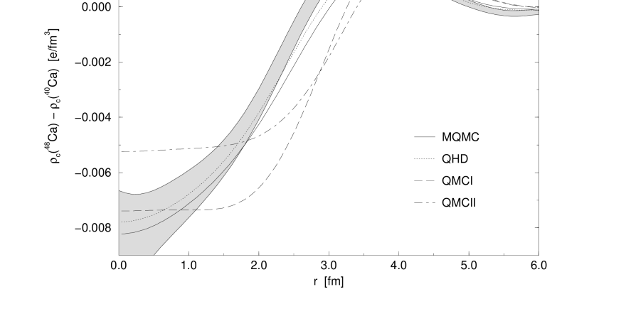
FIG. 7.: Isotope shift in calcium. The difference between the ${}^{48}{\rm Ca}$ and ${}^{40}{\rm Ca}$ charge densities is shown. The experimental (shaded) curve is taken from Ref. [32]. The parameters for the MQMC model are $\eta=4$ and $g_{s}^{q}=3$.

FIG. 8.: Charge density for ${}^{16}{\rm O}$. The parameters for the MQMC model are $\eta=4$ and $g_{s}^{q}=3$.

FIG. 9.: Form factor for ${}^{16}{\rm O}$. The parameters for the MQMC model are $\eta=4$ and $g_{s}^{q}=3$.

FIG. 10.: Single particle spectrum of ${}^{40}{\rm Ca}$. The parameters for the MQMC model are $\eta=4$ and $g_{s}^{q}=3$. The experimental numbers are taken from Ref. [35].

FIG. 11.: Spin-orbit potential for ${}^{40}{\rm Ca}$. The parameters for the MQMC model are $\eta=4$ and $g_{s}^{q}=3$.