On final conditions in high energy heavy ion collisions

Abstract

Motivated by the recent experimental observations, we discuss the freeze-out properties of the fireball created in central heavy ion collisions. We find that the freeze-out conditions, like temperature, velocity gradient near center of the fireball, are similar for different colliding systems and beam energies. This means that the transverse flow is stronger in the collisions of heavy nuclei than that of the light ones.

The system that created in relativistic heavy-ion collision can have both longitudinal and transverse expansion (see, e.g., [1]). In order to study the hadronic experimental data [2, 3], one needs a mathematical description of a final stage of collisions. At the region near mid-rapidity the boundary effect, due to the finite length of the hydrodynamic tube in longitudinal direction, can be neglected [4]. It is possible to use Bjorken’s model for longitudinal expansion: $v_{l}=x_{l}/t$. The same quasi-inertial flow is inherent to Landau model at freeze-out stage [5, 6]. In this approach, the parameter $\tau$ was introduced to describe proper time of the expanding system. For the transverse expansion, we will use a rather general picture proposed in Ref.[7] where, due to the cylindrical symmetry, one has $v_{T}(0)=0$ with the derivative of the transverse velocity near the center of the fireball $v_{T}^{\prime}(0)\neq 0$. The transverse velocity increases monotonously as a function of radius $r$.

The single particle spectra in a pure hydrodynamic picture without resonance decays are expressed by the integral of the Wigner function over the freeze-out surface:

$$p^{0}\frac{d^{3}N}{d^{3}p}=\int d\sigma_{\mu}p^{\mu}f(x,p)$$ (1)

The Wigner function $f(x,p)=f_{th}(x,p)\cdot\rho(x)$, where $f_{th}(x,p)$ is the local thermal distribution function with a temperature parameter $T=1/\beta$, chemical potential $\mu$ and 4-velocity field $u(x)$:

$$f_{th}(x,p)=\frac{(2j+1)}{(2\pi)^{3}}\frac{1}{\exp\left(\beta p^{\mu}u_{\mu}(x)-\beta\mu\right)\mp 1}$$ (2)

The function

$$\rho(x)\propto\exp\left[\frac{\alpha}{2}\left(u(r,y_{L})-u(0,y_{L})\right)^{2}\right]=\exp\left[-\alpha\left(\cosh y_{T}(r)-1\right)\right]$$ (3)

is introduced to describe the finiteness of the relativistically expanding system in transverse direction [7]. Note that the form of the transverse rapidity $y_{T}$ dependent density is similar to one used in Ref. [8]. Here $y_{L}$ and $y_{T}$ are the longitudinal and transverse rapidities respectively and $\alpha$ is the intensity of transverse flows

$$\alpha=(v_{T}^{\prime}(0)\cdot\overline{R}_{T})^{-2}.$$ (4)

For very intensive relativistic transverse flows, $\alpha\rightarrow 0$. On the other hand for $\alpha\gg 1$ we have non-relativistic transverse flows and

$$\rho(x)\propto\exp(-r^{2}/2\overline{R}_{T}^{2})$$ (5)

for $y_{T}(r)\ll 1$.

Using the saddle point approximation , we have obtained from Eq. (1), for $m_{T}\beta\gg 1$, $m_{T}=\sqrt{m^{2}+p_{T}^{2}}$ [7]:

$$\frac{d^{2}N}{m_{T}dm_{T}dy}\propto e^{-(\beta m_{T}+\alpha)(1-\overline{v}_{T}^{2})^{1/2}}$$ (6)

where transverse velocity at the saddle-point $\overline{r}(p)$ is

$$\overline{v}_{T}\equiv\tanh y_{T}(\overline{r}(p))=\frac{\beta p_{T}}{\beta m_{T}+\alpha}$$ (7)

Within the model described in Eqs.(1)-(3), the transverse momentum distribution (6) is not very sensitive to the details of the velocity profile, see Ref. [5]. In the region where

$$m_{T}-m\ll\frac{(\beta m+\alpha)^{2}}{2\beta\alpha}$$ (8)

one has the relationship:

$$(\beta m_{T}+\alpha)(1-\overline{v}_{T}^{2})^{1/2}\cong(\beta m+\alpha)+\frac{\alpha\beta(m_{T}-m)}{(\beta m+\alpha)}$$ (9)

Therefore we have the simplified Eq. (6) as:

$$\frac{d^{2}N}{m_{T}dm_{T}dy}\sim e^{-\beta_{eff}(m_{T}-m)}$$ (10)

with

$$1/\beta_{eff}=T_{eff}=T+\frac{m}{\alpha}.$$ (11)

The latter equation connects the slope of the transverse mass spectra with the intensity of transverse flows

$$\alpha^{1/2}=\frac{\mbox{hydrodynamical length}}{\mbox{transverse radius}}.$$ (12)

The intensity of transverse flows $\alpha$ is defined by the Eq. (4) and does not depend on $m$, it depends only on $A$, where $A$ is the nucleus atomic number.

The system finally decays when the rarefaction wave reaches the center part of the fireball. The analysis of the experimentally measured slope parameters ($T_{eff}$) as a function of particle mass [10] with two parameters, $T$ and $\alpha,$ shows that the freeze-out temperature $T$ is approximately constant for different colliding systems at the beam energy $\geq$ 10A$\cdot$GeV. Hence it is natural to conclude that the physical condition near the center is the same for different colliding systems, i.e. $v_{T}^{\prime}(0)$ is constant. From Eq.(4) we obtain

$$v_{T}^{\prime}(0)=(\alpha\overline{R}_{T}^{2})^{-1/2}$$ (13)

In our approach $\overline{R}_{T}$ is the Gaussian-like radius of a decaying system. We suppose that $\overline{R}_{T}$ depends on $A$ only. It means that in the same collisions a freeze-out “size” is unique for different particle species. The value $\overline{R}_{T}$ is connected with the so called sideward radius $R_{s}$ [11], obtained from the fit of the experimentally measured two-particle correlation functions, in the following way. When $\overline{v}_{T}=\frac{\beta p_{T}}{\beta m_{T}+\alpha}\ll$ 1 (non-relativistic approximation) it can be shown that only $v_{T}^{\prime}(0)$ has an influence on the interferometry radii and any details of the transverse velocity profile $v_{T}(r)=\tanh y_{T}(r)$ are not important [7, 12]. Within this approximation, one has the following expression for the Gaussian transversal sideward radius [7, 12]:

$$\overline{R}_{T}\sqrt{\frac{\alpha}{\beta m_{T}+\alpha}}=R_{S}(p_{T}).$$ (14)

From this equation we evaluate $\overline{R}_{T}$, using experimental data for $R_{S}(p_{T})$, and $\beta$ and $\alpha$ from the fitting procedure [10] based on Eq. (11). To minimize the influence of the resonance decays, the interferometry radius for every analyzed particle species has to be measured at the point where $p_{T}$ is large enough. On the other hand, in order to provide a validity of the non-relativistic approximation and the correctness of the condition Eq. (8), the value of $p_{T}$ should be limited with $\overline{v}_{T}\ll 1$.

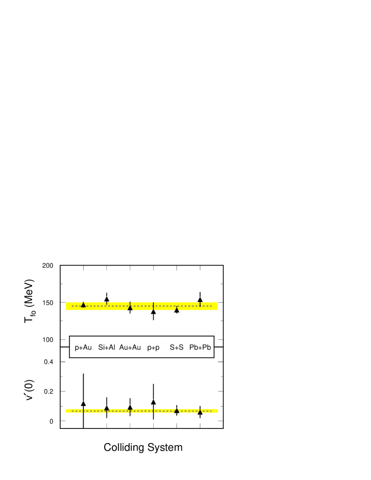
Figure 1: The freeze-out temperature $T$ (top) and flow velocity gradient (bottom) calculated at $r\approx$ 0. The set of data for this calculation is the taken from the references listed in Table I.

Using the experimental data, listed in Table I, we evaluate the freeze-out temperature and velocity gradient at the center of the fireball. The results of the fit are shown in Fig. 1. Note that there are two important features in the plot. First, the values of the intrinsic temperature $T$ seems to be a constant (top plot of Fig. 1). It does not dependent on the size of colliding system. Furthermore, for collisions at the AGS energies (11 - 15 A$\cdot$GeV/c) and SPS energies (158 - 200 A$\cdot$GeV/c), this parameter is approximately the same. Secondly, the value $v_{T}^{{}^{\prime}}(0)$ is also closed to a constant (see bottom plot of Fig. 1).

It has been noted that the temperature is limited for collisions at beam energies larger than 11 A$\cdot$GeV (Fig. 2 of Ref. [10]). One should note that, although we do not observe the difference in $v_{T}^{{}^{\prime}}(0)$ between the collisions at AGS and SPS energies, it is quite possible that at lower beam energies one gets somewhat different values. The saturation of the freeze-out temperature might reflect the limiting temperature hypothesis pointed by Hagedorn some years ago [15, 16]. On the other hand, the constant behavior of the velocity gradient near the center of the fireball is a new result yield by the present study. It clearly shows that at the final stage, the freeze-out conditions are approximately the same for different size and different beam energies of the collisions. Constant transverse velocity gradient actually means that both the averaged transverse velocity and flow intensity grow with the size of the colliding nuclei. Indeed, the average transverse hydrodynamic velocity that can be calculated using the final distribution function (2) is

$$\left\langle v_{T}\right\rangle=\frac{\int\frac{d^{3}p}{p^{0}}\int d\sigma_{\mu}p^{\mu}v_{T}(x)f(x,p)}{\int\frac{d^{3}p}{p^{0}}\int d\sigma_{\mu}p^{\mu}f(x,p)}=\frac{\int d\sigma_{\mu}u^{\mu}(x)\rho(x)v_{T}(x)}{\int d\sigma_{\mu}u^{\mu}(x)\rho(x)}$$ (15)

For $\tau(r)\cong const$ at the freeze-out hypersurface we can get from Eq. (15):

$$\left\langle v_{T}\right\rangle\cong\frac{\int\tanh y_{T}(r)\cosh y_{T}(r)\exp\left[-\alpha\cosh y_{T}(r)\right]rdr}{\int\cosh y_{T}(r)\exp\left[-\alpha\cosh y_{T}(r)\right]rdr}.$$ (16)

Using saddle point approximation, in the limit of $\alpha\gg 1$, one can show that the average transverse hydrodynamic velocity is

$$\left\langle v_{T}\right\rangle \cong v_{T}^{\prime}(0)\frac{\int\exp(-r^{2}/2\overline{R}_{T}^{2})r^{2}dr}{\int\exp(-r^{2}/2\overline{R}_{T}^{2})rdr}\cong$$

$$\cong \sqrt{\frac{\pi}{2}}v_{T}^{\prime}(0)\overline{R}_{T}=\sqrt{\frac{\pi}{2\alpha}}$$

Let us note that $\overline{v}_{T}\neq\left\langle v_{T}\right\rangle$. The physical meaning is that, in the saddle point approximation, $\overline{v}_{T}$ is the transverse velocity of the fluid element which gives the main contribution to transverse momentum spectrum at given $p_{T}$. On the other hand, $\left\langle v_{T}\right\rangle$ is the averaged transverse hydrodynamic velocity that characterizes whole system. From Eqs. (16) and (17), one can see that $\alpha$ is directly connected with $\left\langle v_{T}\right\rangle$. So we find that, in approximation of Eq. (17), the averaged values of the transverse velocity $\langle v_{T}\rangle$ are 0.49$c$ and 0.33$c$ for Pb+Pb and S+S central collisions [10], respectively. Formally the averaged velocity $\langle v_{T}\rangle$ is consistent with zero for p+p collisions although the application of the thermal model for such collisions remains an open question. At the freeze-out surface, the effective slopes of spectra for different colliding systems and different mass particle species can be presented by the non-relativistic average transverse hydrodynamic velocity:

$$T_{eff}\approx T+\frac{2}{\pi}m\left\langle v_{T}\right\rangle^{2}.$$ (18)

The merit of this equation is that by fitting the measured slope parameter as a function of particle mass, one can separate the collective motion from the thermal motion. Therefore, the intrinsic freeze-out temperature $T$ and averaged collective velocity $\langle v_{T}\rangle$ can be readily extracted from the data. The measured slope parameters of pions, kaons, and protons [10] seem to obey the linear mass dependence as given by Eq. (18). One new finding from this study is the linear tie of the averaged transverse velocity $\langle v_{T}\rangle$ with the radius $\overline{R}_{T}$, see Eq. (17). It is worth mentioning that the hydrodynamic arguments for the behavior of the slope parameter as a function of a particle mass is valid as long as the considered particle species remain a part of the fireball and hence are participating in the frequent rescatterings. For those particles with high probability of destruction, such description is not valid anymore. It is possible that those particles freeze-out earlier than the other hadrons which participate in the evolution of the system longer. They do not have enough time to acquire a common collective velocity and hence the corresponding slope parameters could be smaller than the predicted by Eq. (18). Indeed, the recent preliminary results reported by WA97 [17] and NA49 [18] show such deviations for hyperons, particularly for $\Omega$ particle [19]. In order to understand the dynamics involved for those particles, one has to take the collision rate for individual considered particle into account.

In summary, using a thermal model we analyzed the recent experimental data from heavy ion collisions. We found that the freeze-out temperature is a constant for all colliding systems at $E_{beam}>$10 A$\cdot$GeV and a constant velocity gradient at the center of the fireball ($r\rightarrow 0$).

Acknowledgments: One of us (Nu Xu) wishes to thank Professor H. Stöcker for many helpful discussions on the physics of thermalization and hydrodynamic flow in heavy-ion collisions. We thank Dr. S. Panitkin for careful reading of the manuscript. We gratefully acknowledges support by the Ukrainian State Fund of the Fundamental Research under Contract No 2.5.1/057 and by the U.S. Department of Energy under Contract No. DE-AC03-76SF00098.

System	1/$\sqrt{\alpha}$	$R_{S}$
p + p [10]	0.01$\pm$0.11	0.8$\pm$0.2
S + S [10]	0.26$\pm$0.10	2.9$\pm$0.2
Pb + Pb [10]	0.39$\pm$0.12	5.1$\pm$0.4
Si + Al [13]	0.29$\pm$0.12	2.56$\pm$0.17
Si + Au [13]	0.30$\pm$0.12	2.4$\pm$1.1
Au + Au [14]	0.42$\pm$0.11	3.57$\pm$0.52

Table 1: Experimental transverse velocity intensity and sideward radius parameters for different colliding systems. Error bars are statistical only. Note that for the AGS energies, the size parameters $R_{S}$ is taken from 2-dimensional fits assuming that $R_{T}=R_{S}$. All size parameters are obtained with a cut $p_{T}>$ 0.2 GeV/c.

References

- [1] E. Schnedermann, J. Sollfrank, and U. Heinz, Phys. Rev. C48, 2462 (1993).
- [2] S. Pratt and J. Murray, Phys. Rev. C57, 1907(1998).
- [3] J.R. Nix et al., in Advances in Nuclear Dynamics 4, Proc. 14th Winter Workshop on Nuclear Dynamics, Snowbird, Utah, 1998 (Plenum Press, New York, 1998).
- [4] V.A. Averchenkov, A.N. Makhlin, Yu.M. Sinyukov, Sov.J.Nucl.Phys. 46, 905 (1987).
- [5] L.D. Landau, Izv. Akad. Nauk SSSR Ser. Fiz. 17, 51 (1953).
- [6] J.D. Bjorken, Phys. Rev. D27, 140 (1983).
- [7] S.V. Akkelin and Yu.M. Sinyukov, Phys. Lett. B356, 525 (1995); S.V. Akkelin and Yu.M. Sinyukov, Z. Phys. C72, 501 (1996).
- [8] A. Leonidov, M. Nardi and H. Satz, Nucl. Phys. A610, 124c (1996).
- [9] T. Csorgo, B. Lorstad, J. Zimanyi, Phys. Lett. B338, 134 (1994).
- [10] I.G. Bearden et al., (The NA44 Collaboration), Phys. Rev. Lett. 78, 2080 (1996).
- [11] S. Pratt, Phys. Rev. D33, 1314(1986).
- [12] Yu.M. Sinyukov, S.V. Akkelin, A.Yu. Tolstykh, Nucl. Phys. A610, 278c (1996).
- [13] V. Cianciolo, Nucl. Phys. A590, 459c(1995).
- [14] M.D. Baker, Nucl. Phys. A610, 213c(1996).
- [15] R. Hagedorn, Suppl. Nuovo Cim. III.2, 147 (1965).
- [16] H. Stöcker, A.A. Ogloblin, and W. Greiner, Z. Phys. A303, 259 (1981).
- [17] I. Kralik et al., (The WA97 Collaboration), Quark Matter ’97, Tsukuba, Japan, Dec. 1 - 5, 1997.
- [18] G. Roland et al., (The NA49 Collaboration), Quark Matter ’97, Tsukuba, Japan, Dec. 1 - 5, 1997.
- [19] H. van Hecke, H. Sorge, N. Xu, submitted to Phys. Rev. Lett., April 1998.