Pseudovector components of the pion, $\pi^{0}\to\gamma\gamma$, and $F_{\pi}(q^{2})$

Abstract

As a consequence of dynamical chiral symmetry breaking the pion Bethe-Salpeter amplitude necessarily contains terms proportional to $\gamma_{5}\,\gamma\cdot P$ and $\gamma_{5}\,\gamma\cdot k$, where $k$ is the relative and $P$ the total momentum of the constituents. These terms are essential for the preservation of low energy theorems, such as the Gell-Mann–Oakes-Renner relation and those describing anomalous decays of the pion, and to obtaining an electromagnetic pion form factor that falls as $1/q^{2}$ for large $q^{2}$, up to calculable $\ln q^{2}$-corrections. In a simple model, which correlates low- and high-energy pion observables, we find $q^{2}F_{\pi}(q^{2})\sim 0.12$ - $0.19\,$GeV² for $q^{2}\mathrel{\hbox to0.0pt{\lower 4.0pt\hbox{\hskip 0.0pt$\sim$}\hss}\raise 2.0pt\hbox{$>$}}10\,{\rm GeV}^{2}$.

I Pion as a bound state

Understanding the pion is a key problem in strong interaction physics. As the lowest mass excitation in the strong interaction spectrum it must provide the long-range attraction in $N$-$N$ potentials [1]. In QCD, it is a quark-antiquark bound state whose low- and high-energy properties should be understandable in terms of its internal structure, and it is also that nearly-massless, collective excitation which is the realisation of the Goldstone mode associated with dynamical chiral symmetry breaking (DCSB). An explanation of these properties requires a melding of the study of the many body aspects of the QCD vacuum with the analysis of two body bound states. The Dyson-Schwinger equations (DSEs) provide a single, Poincaré invariant framework that is well suited to this problem.

The DSEs are a system of coupled integral equations and truncations are employed to define a tractable problem. In truncating the system it is straightforward to preserve the global symmetries of a gauge field theory [2] and, although preserving the local symmetry is more difficult, progress is being made [3]. The approach has been applied extensively [4] to the study of confinement, and to DCSB where the similarity between the ground state of QCD and that of a superconductor can be exploited, with the QCD gap equation realised as the quark DSE. It has also been employed in studying meson-meson and meson-photon interactions [5], heavy meson decays [6], QCD at finite temperature and density [7], and strong interaction contributions to weak interaction phenomena [8, 9].

Studying the pion as a bound state requires an understanding of its (fully-amputated) Bethe-Salpeter amplitude, which has the general form

$$\Gamma_{\pi}^{j}(k;P) = \tau^{j}\gamma_{5}\left[iE_{\pi}(k;P)+\gamma\cdot PF_{\pi}(k;P)\rule{0.0pt}{14.22636pt}\right.$$ (2)

$$\left.\rule{0.0pt}{14.22636pt}+\gamma\cdot k\,k\cdot P\,G_{\pi}(k;P)+\sigma_{\mu\nu}\,k_{\mu}P_{\nu}\,H_{\pi}(k;P)\right]\,,$$

where $\{\tau^{j}\}_{j=1\ldots 3}$ are the Pauli matrices. $\Gamma_{\pi}^{j}$ satisfies the renormalised, homogeneous Bethe-Salpeter equation

$$\left[\Gamma_{\pi}^{j}(k;P)\right]_{tu} = \int^{\Lambda}_{q}\,[\chi_{\pi}^{j}(q;P)]_{sr}\,K^{rs}_{tu}(q,k;P)\,,$$ (3)

where $k$ is the relative and $P$ the total momentum of the quark-antiquark pair, $\chi_{\pi}^{j}(q;P):=S(q_{+})\Gamma_{\pi}^{j}(q;P)S(q_{-})$, $r$,…,$u$ represent colour, flavour and Dirac indices, $q_{\pm}=q\pm P/2$, and $\int^{\Lambda}_{q}:=\int^{\Lambda}d^{4}q/(2\pi)^{4}$ represents mnemonically a translationally-invariant regularisation of the integral, with $\Lambda$ the regularisation mass-scale: $\Lambda\to\infty$ is the last step in any calculation. In Eq. (3), $K$ is the fully-amputated, renormalised quark-antiquark scattering kernel and $S$ is the renormalised dressed-quark propagator, which is the solution of

$$S(p)^{-1} = Z_{2}(i\gamma\cdot p+m_{\rm bm})+\,Z_{1}\int^{\Lambda}_{q}\,g^{2}D_{\mu\nu}(p-q)\gamma_{\mu}S(q)\Gamma_{\nu}(q,p)\,,$$ (4)

where $D_{\mu\nu}(k)$ is the renormalised dressed-gluon propagator, $\Gamma_{\mu}(q;p)$ is the renormalised dressed-quark-gluon vertex and $m_{\rm bm}(\Lambda)$ is the Lagrangian current-quark bare mass. In Eq. (4), $Z_{1}$ and $Z_{2}$ are the renormalisation constants for the quark-gluon vertex and quark wave function, and the chiral limit is obtained with $m_{\rm bm}(\Lambda)=0$. The solution of Eq. (4) has the general form

$$S(p) = -i\gamma\cdot p\,\sigma_{V}(p^{2})+\sigma_{S}(p^{2})\equiv\frac{1}{i\gamma\cdot p\,A(p^{2})+B(p^{2})}\,.$$ (5)

Also important in the study of the pion is the chiral-limit, axial-vector Ward-Takahashi identity

$$-iP_{\mu}\Gamma_{5\mu}^{j}(q;P)=S^{-1}(q_{+})\,\gamma_{5}\frac{\tau^{j}}{2}+\gamma_{5}\frac{\tau^{j}}{2}\,S^{-1}(q_{-})\,.$$ (6)

This identity relates the renormalised, dressed-quark propagator to the renormalised axial-vector vertex, which satisfies

$$\left[\Gamma_{5\mu}^{j}(k;P)\right]_{tu} = Z_{2}\,\left[\gamma_{5}\gamma_{\mu}\frac{\tau^{j}}{2}\right]_{tu}\,+\int^{\Lambda}_{q}\,[\chi_{5\mu}^{j}(q;P)]_{sr}\,K^{rs}_{tu}(q,k;P)\,,$$ (7)

where $\chi_{5\mu}^{j}(q;P):=S(q_{+})\Gamma_{5\mu}^{j}(q;P)S(q_{-})$. In the chiral limit the general solution of Eq. (7) is [10, 11]

$$\Gamma_{5\mu}^{j}(k;P) = \frac{\tau^{j}}{2}\gamma_{5}\left[\rule{0.0pt}{14.22636pt}\gamma_{\mu}F_{R}(k;P)+\gamma\cdot kk_{\mu}G_{R}(k;P)-\sigma_{\mu\nu}\,k_{\nu}\,H_{R}(k;P)\right]$$ (8)

$$+ \tilde{\Gamma}_{5\mu}^{j}(k;P)+\,f_{\pi}^{0}\,\frac{P_{\mu}}{P^{2}}\,\Gamma_{\pi}(k;P)\,,$$ (9)

where: $F_{R}$, $G_{R}$, $H_{R}$ and $\tilde{\Gamma}_{5\mu}^{j}$ are regular as $P^{2}\to 0$; $P_{\mu}\tilde{\Gamma}_{5\mu}^{j}(k;P)\sim{\rm O}(P^{2})$; $\Gamma_{\pi}(k;P)$ is the amplitude in Eq. (2); and the residue of the pole in the axial-vector vertex is $f_{\pi}^{0}$, the chiral-limit leptonic decay constant, which is obtained from:

$$\delta^{ij}f_{\pi}P_{\mu}=Z_{2}\int^{\Lambda}_{q}\,{\rm tr}\left[\frac{\tau^{i}}{2}\gamma_{5}\gamma_{\mu}S(q_{+})\Gamma_{\pi}^{j}(q;P)S(q_{-})\right]\,.$$ (10)

[This expression is valid for arbitrary values of the quark mass.] Now, independent of assumptions about the the form of $K$, it follows [10] from Eqs. (5), (6) and (8) that

$$f_{\pi}^{0}E_{\pi}(k;0) = B_{0}(k^{2})\,,$$ (11)

$$F_{R}(k;0)+2\,f_{\pi}^{0}F_{\pi}(k;0) = A_{0}(k^{2})\,,$$ (12)

$$G_{R}(k;0)+2\,f_{\pi}^{0}G_{\pi}(k;0) = 2A_{0}^{\prime}(k^{2})\,,$$ (13)

$$H_{R}(k;0)+2\,f_{\pi}^{0}H_{\pi}(k;0) = 0\,,$$ (14)

where $A_{0}$ and $B_{0}$ are the chiral limit solutions of Eq. (4). A necessary consequence of Eqs. (11)-(14) is that the pseudovector components $F_{\pi}$ and $G_{\pi}$, and the pseudotensor component $H_{\pi}$, are nonzero in Eq. (2). This corrects a misapprehension [12] that only $E_{\pi}\neq 0$ and has important phenomenological consequences.

A Normalisation of the pion field

To highlight one such consequence we note that Eq. (3), the homogeneous Bethe-Salpeter equation, does not determine the normalisation of the Bethe-Salpeter amplitude. The canonical normalisation is fixed by requiring that the pion pole in the quark-antiquark scattering amplitude: $M:=K/[1-(SS)K]$, have unit residue. As an alternative, one can normalise the solution of Eq. (3) by requiring that $E(0;0)=B(0)$ in the chiral limit. In terms of the amplitude ${\cal G}_{\pi}(k;P)$ defined in this way, the canonical normalisation condition is

$$2\delta^{ij}N_{\pi}^{2}\,P_{\mu}=\int^{\Lambda}_{q}\left\{\rule{0.0pt}{14.22636pt}{\rm tr}\left[\bar{\cal G}_{\pi}^{i}(q;-P)\frac{\partial S(q_{+})}{\!\!\!\!\!\!\partial P_{\mu}}{\cal G}_{\pi}^{j}(q;P)S(q_{-})\right]\right.$$ (17)

$$\left.\;\;\;\;\;\;\;\;\;\;\;\;\;\;\;\;\;\;\;+{\rm tr}\left[\bar{\cal G}_{\pi}^{i}(q;-P)S(q_{+}){\cal G}_{\pi}^{j}(q;P)\frac{\partial S(q_{-})}{\!\!\!\!\!\!\partial P_{\mu}}\right]\rule{0.0pt}{14.22636pt}\right\}$$

$$\;\;\;\;\;\;\;\;\;\;+\int^{\Lambda}_{q}\int^{\Lambda}_{k}\,[\bar{\chi}_{{\cal G}_{\pi}}^{i}(q;-P)]_{sr}\frac{\partial K^{rs}_{tu}(q,k;P)}{\!\!\!\!\!\!\!\!\!\!\!\!\partial P_{\mu}}\,[\chi_{{\cal G}_{\pi}}^{j}(k;P)]_{ut}\,,$$

where $\bar{\cal G}_{\pi}(q;-P)^{t}:=C^{-1}\,{\cal G}_{\pi}(-q;-P)\,C$ with $C=\gamma_{2}\gamma_{4}$, the charge conjugation matrix, and $X^{t}$ denoting the matrix transpose of $X$. Equation (17) defines the pion normalisation constant, $N_{\pi}$, which has mass-dimension one. Physical observables are expressed in terms of $\Gamma_{\pi}(k;P):=(1/N_{\pi})\,{\cal G}_{\pi}(k;P)$.

In the chiral limit, when all the amplitudes in Eq. (2) are retained, one obtains [10]

$$f_{\pi}^{0}=N_{\pi}^{0}\,.$$ (18)

This result verifies a core assumption in chiral perturbation theory; i.e., that the pion field is normalised by $f_{\pi}^{0}$, which is implicit in the expression of the chiral field as

$$U(x):={\rm e}^{i\vec{\tau}\cdot\vec{\pi}(x)/f_{\pi}^{0}}\,.$$ (19)

However, Eq. (18) is violated in bound state treatments of the pion that neglect the pseudovector components of the Bethe-Salpeter amplitude [11].

II Anomalous Neutral Pion Decay

The pseudovector components of the pion also play a special role in the anomalous $\pi^{0}\to\gamma\gamma$ decay. Consider the renormalised, impulse approximation to the axial-vector–photon-photon (AVV) amplitude:

$${\cal T}_{\rho\mu\nu}(k_{1},k_{2}) := T_{\rho\mu\nu}(k_{1},k_{2})+T_{\rho\nu\mu}(k_{2},k_{1})\,,$$ (20)

$$T_{\rho\mu\nu}(k_{1},k_{2}) := N_{c}\int^{\Lambda}_{q}\left\{{\rm tr}_{DF}\left[\rule{0.0pt}{12.0pt}S(q_{1})\,\Gamma_{5\rho}^{3}(\hat{q};-P)\,S(q_{2})\,i\Gamma^{\gamma}_{\mu}(q_{2},q_{12})S(q_{12})\,i\Gamma^{\gamma}_{\nu}(q_{12},q_{1})\right]\right\}\,,$$ (21)

where $k_{1}$, $k_{2}$ are the photon momenta [$k_{1}^{2}=0=k_{2}^{2}$, $2k_{1}\cdot k_{2}=P^{2}$], $q$ is the loop-momentum, and $q_{1}:=q-k_{1}$, $q_{2}:=q+k_{2}$, $\hat{q}:=\frac{1}{2}(q_{1}+q_{2})$, $q_{12}:=q-k_{1}+k_{2}$.

Here $\Gamma^{\gamma}_{\mu}(p_{1},p_{2})$ is the renormalised, dressed-quark-photon vertex, and it is because this vertex satisfies the vector Ward-Takahashi identity:

$$(p_{1}-p_{2})_{\mu}\,i\Gamma^{\gamma}_{\mu}(p_{1},p_{2})=S^{-1}(p_{1})-S^{-1}(p_{2})\,,$$ (22)

that no renormalisation constants appear explicitly in Eq. (21). $\Gamma^{\gamma}_{\mu}(p_{1},p_{2})$ has been much studied [3] and, although its exact form remains unknown, its robust qualitative features have been elucidated so that a phenomenologically efficacious Ansatz has emerged [13]

$$i\Gamma^{\gamma}_{\mu}(p,q) := i\Sigma_{A}(p^{2},q^{2})\,\gamma_{\mu}+(p+q)_{\mu}\,\left[\frac{1}{2}i\gamma\cdot(p+q)\,\Delta_{A}(p^{2},q^{2})+\Delta_{B}(p^{2},q^{2})\right]\,;$$ (23)

$$\Sigma_{f}(p^{2},q^{2}) := \frac{1}{2}\,[f(p^{2})+f(q^{2})]\,,$$ (24)

$$\Delta_{f}(p^{2},q^{2}) := \frac{f(p^{2})-f(q^{2})}{p^{2}-q^{2}}\,,$$ (25)

where $f=A,B$. A feature of Eq. (23) is that the vertex is completely determined by the renormalised dressed-quark propagator. In Landau gauge the quantitative effect of modifications, such as that canvassed in Ref. [19], is small and can be compensated for by small changes in the parameters that characterise a given model study [20].

In the chiral limit ($P^{2}=0$) using Eqs. (2) and (8), the divergence of the AVV vertex is

$$P_{\rho}\,T_{\rho\mu\nu}(k_{1},k_{2}) = R^{3}_{\mu\nu}(k_{1},k_{2})+f_{\pi}^{0}\,T^{3}_{\mu\nu}(k_{1},k_{2})\,,$$ (26)

where the direct contribution from the axial-vector vertex is

$$R^{3}_{\mu\nu}(k_{1},k_{2}):=-N_{c}\int^{\Lambda}_{q}{\rm tr}_{DF}\left[\rule{0.0pt}{12.0pt}S(q_{1})\,\gamma_{5}\frac{\tau^{3}}{2}\left(\rule{0.0pt}{12.0pt}\gamma\cdot P\,F_{R}(\hat{q};0)\right.\right.$$ (28)

$$\left.\left.+\gamma\cdot\hat{q}\,\hat{q}\cdot P\,G_{R}(\hat{q};0)+\sigma_{\mu\nu}\,\hat{q}_{\mu}P_{\nu}\,H_{R}(\hat{q};0)\rule{0.0pt}{12.0pt}\right)S(q_{2})\,i\Gamma^{\gamma}_{\mu}(q_{2},q_{12})S(q_{12})\,i\Gamma^{\gamma}_{\nu}(q_{12},q_{1})\rule{0.0pt}{12.0pt}\right]\,,$$

and that from the pion bound state is

$$T^{3}_{\mu\nu}(k_{1},k_{2}):=N_{c}\int^{\Lambda}_{q}{\rm tr}_{DF}\left[\rule{0.0pt}{12.0pt}S(q_{1})\,\gamma_{5}\tau^{3}\left(\rule{0.0pt}{12.0pt}iE_{\pi}(\hat{q};0)-\gamma\cdot P\,F_{\pi}(\hat{q};0)\right.\right.$$ (30)

$$\left.\left.-\gamma\cdot\hat{q}\,\hat{q}\cdot P\,G_{\pi}(\hat{q};0)-\sigma_{\mu\nu}\,\hat{q}_{\mu}P_{\nu}\,H_{\pi}(\hat{q};0)\rule{0.0pt}{12.0pt}\right)S(q_{2})\,i\Gamma^{\gamma}_{\mu}(q_{2},q_{12})S(q_{12})\,i\Gamma^{\gamma}_{\nu}(q_{12},q_{1})\rule{0.0pt}{12.0pt}\right]\,.$$

Using Eqs. (12)-(14), Eq. (26) simplifies:

$$P_{\rho}\,T_{\rho\mu\nu}(k_{1},k_{2})=\hat{R}^{3}_{\mu\nu}(k_{1},k_{2})+f_{\pi}^{0}\,\hat{T}^{3}_{\mu\nu}(k_{1},k_{2})\,;$$ (31)

$$\hat{R}^{3}_{\mu\nu}(k_{1},k_{2}):=-N_{c}\int^{\Lambda}_{q}{\rm tr}_{DF}\left[\rule{0.0pt}{12.0pt}S(q_{1})\,\gamma_{5}\frac{\tau^{3}}{2}\left(\rule{0.0pt}{12.0pt}\gamma\cdot P\,A_{0}(\hat{q}^{2})\right.\right.$$ (33)

$$\left.\left.+\gamma\cdot\hat{q}\,\hat{q}\cdot P\,2A_{0}^{\prime}(\hat{q}^{2})\right)S(q_{2})\,i\Gamma^{\gamma}_{\mu}(q_{2},q_{12})S(q_{12})\,i\Gamma^{\gamma}_{\nu}(q_{12},q_{1})\rule{0.0pt}{12.0pt}\right]\,,$$

$$\hat{T}^{3}_{\mu\nu}(k_{1},k_{2}) := N_{c}\int^{\Lambda}_{q}{\rm tr}_{DF}\left[\rule{0.0pt}{12.0pt}S(q_{1})\,\gamma_{5}\tau^{3}\,iE_{\pi}(\hat{q};0)\,S(q_{2})\,i\Gamma^{\gamma}_{\mu}(q_{2},q_{12})S(q_{12})\,i\Gamma^{\gamma}_{\nu}(q_{12},q_{1})\right]\,.$$ (34)

Now using Eqs. (5) and (23) in Eq. (33) yields

$$\hat{R}^{3}_{\mu\nu}(k_{1},k_{2})=\,-\,\frac{\alpha_{\rm em}}{\pi}\,\epsilon_{\mu\nu\rho\sigma}k_{1\rho}k_{2\sigma}\,{\cal R}(P^{2}=0)$$ (35)

where ($s:=q^{2}$, $A_{0}^{\prime}:=\frac{d}{ds}A_{0}(s)$, etc.),

$${\cal R}(0) = \int_{0}^{\infty}\,ds\,s^{2}\,A_{0}^{2}\,\sigma_{V}^{0}\,\left(A_{0}\left[(\sigma_{V}^{0})^{2}+s\,\sigma_{V}^{0}\,\sigma_{V}^{0\,\prime}+\sigma_{S}^{0\,\prime}\,\sigma_{S}^{0}\right]+\sigma_{V}^{0}\left[sA_{0}^{\prime}\,\sigma_{V}^{0}+B_{0}^{\prime}\,\sigma_{S}^{0}\right]\right)$$ (36)

$$\equiv 0\,.$$ (37)

The last line follows because, using Eq. (5) to eliminate $\sigma_{V}^{0}$ and $\sigma_{S}^{0}$ in favour of $A_{0}$ and $B_{0}$, the integrand is identically zero. Hence the pseudovector components of the neutral-pion Bethe-Salpeter amplitude combine with the regular pieces of the axial-vector vertex to generate that part of the AVV vertex which is conserved.

To reveal the anomalous contribution to the divergence, consider Eq. (34), in which using Eqs. (5) and (23) yields

$$\hat{T}^{3}_{\mu\nu}(k_{1},k_{2})=\frac{\alpha_{\rm em}}{\pi}\,\epsilon_{\mu\nu\rho\sigma}k_{1\rho}k_{2\sigma}\,{\cal T}(0)\,,$$ (38)

$${\cal T}(0) = \int_{0}^{\infty}\,ds\,s\,E_{\pi}\,A_{0}\,\sigma_{V}^{0}\,\left(A_{0}\left[\sigma_{V}^{0}\,\sigma_{S}^{0}+s\left(\sigma_{V}^{0\,\prime}\,\sigma_{S}^{0}-\sigma_{V}^{0}\,\sigma_{S}^{0\,\prime}\right)+s\,\sigma_{V}^{0}\,\left(A_{0}^{\prime}\,\sigma_{S}^{0}-B_{0}^{\prime}\,\sigma_{V}^{0}\right)\right]\right)\,.$$ (39)

Now, introducing $C(s):=B_{0}(s)^{2}/[sA_{0}(s)^{2}]$, Eq. (39) simplifies

$${\cal T}(P^{2}=0)=-\int_{0}^{\infty}\,ds\,s\,\frac{E_{\pi}(s;0)}{B_{0}(s)}\,\frac{C^{\prime}(s)}{[1+C(s)]^{3}}\,,$$ (40)

which, using Eq. (11), yields

$$f_{\pi}^{0}\,{\cal T}(P^{2}=0)=\int_{0}^{\infty}\,dC\,\frac{1}{(1+C)^{3}}=\frac{1}{2}\,,$$ (41)

so that, in the chiral limit,

$$P_{\rho}\,{\cal T}_{\rho\mu\nu}(k_{1},k_{2})=\frac{\alpha_{\rm em}}{\pi}\,\epsilon_{\mu\nu\rho\sigma}k_{1\rho}k_{2\sigma}\,.$$ (42)

Hence the pseudoscalar piece of the neutral-pion Bethe-Salpeter amplitude provides the only nonzero contribution to the divergence of the AVV amplitude. This contribution is just that identified with the “triangle anomaly”, and the result is independent of detailed information about $\Gamma_{\pi}$ and $S(p)$. It follows straightforwardly from Eqs. (38) and (41) that

$$\Gamma_{\pi^{0}\to\gamma\gamma}=\frac{m_{\pi}^{3}}{16\pi}\frac{\alpha^{2}_{\rm em}}{\pi^{2}}\,{\cal T}(0)^{2}=\frac{m_{\pi}^{3}}{64\pi}\left(\frac{\alpha_{\rm em}}{\pi\,f_{\pi}^{0}}\right)^{2}\,.$$ (43)

We emphasise that in obtaining the results in this section DCSB was crucial, since it originates and is manifest in a nonzero value of $B_{0}$, in the identity between $B_{0}$ and $E_{\pi}$, and in the other identities: Eqs. (12)-(14).

Our derivation is a generalisation of that in Ref. [14] and, to make it simple, particular care was taken in choosing the momentum routing in Eq. (21). This was necessary because it is impossible to simultaneously preserve the vector and axial vector Ward-Takahashi identities for triangle diagrams in field theories with axial currents that are bilinear in fermion fields. This choice of variables ensures the preservation of the vector Ward-Takahashi identity, which is tied to electromagnetic current conservation. With another choice of variables, surface terms arise that modify the value of ${\cal R}(P^{2}=0)$. However, these are always eliminated by subtraction in any regularisation of the theory that ensures electromagnetic current conservation.[15]

III Electromagnetic pion form factor

As another example of the importance of $\Gamma_{\pi}$’s pseudovector components, we consider the electromagnetic pion form factor, calculated in the renormalised impulse approximation:

$$(p_{1}+p_{2})_{\mu}\,F_{\pi}(q^{2}):=\Lambda_{\mu}(p_{1},p_{2})$$ (45)

$$=\frac{2N_{c}}{N_{\pi}^{2}}\,\int\,\frac{d^{4}k}{(2\pi)^{4}}\,{\rm tr}_{D}\left[\bar{\cal G}_{\pi}(k;-p_{2})S(k_{++})\,i\Gamma^{\gamma}_{\mu}(k_{++},k_{+-})\,S(k_{+-})\,{\cal G}_{\pi}(k-q/2;p_{1})\,S(k_{--})\right],$$

$k_{\alpha\beta}:=k+\alpha p_{1}/2+\beta q/2$ and $p_{2}:=p_{1}+q$. Again, no renormalisation constants appear explicitly in Eq. (45) because the renormalised dressed-quark-photon vertex, $\Gamma^{\gamma}_{\mu}$, satisfies the vector Ward-Takahashi identity, Eq. (22). This also ensures current conservation:

$$(p_{1}-p_{2})_{\mu}\,\Lambda_{\mu}(p_{1},p_{2})=0\,.$$ (46)

We note that from the normalisation condition for ${\cal G}_{\pi}$, Eq. (17), and Eqs. (22) and (45)

$$F(q^{2}=0)=1$$ (47)

if, and only if, one employs a truncation in which $K$ is independent of $P$. One such scheme is the rainbow-ladder truncation of Ref. [11].

A Quark propagator

To calculate $F_{\pi}(q^{2})$ we employ an algebraic parametrisation of the renormalised dressed-quark propagator that efficiently characterises many essential and robust elements of the solutions obtained in studies of the quark DSE. This defines Eq. (45) directly $\forall\,p_{1}^{2},p_{2}^{2}$; in particular at the pion mass shell. We introduce the dimensionless functions: $\bar{\sigma}_{S}(x):=\lambda\,\sigma_{S}(p^{2})$, $\bar{\sigma}_{V}(x):=\lambda^{2}\,\sigma_{V}(p^{2})$, where $p^{2}=\lambda^{2}\,x$, $\lambda$ is a mass-scale, with

$$\bar{\sigma}_{S}(\xi) = 2\bar{m}{\cal F}(2(\xi+\bar{m}^{2}))+{\cal F}(b_{1}\,\xi){\cal F}(b_{3}\,\xi)\left(b_{0}+b_{2}{\cal F}(\varepsilon\,\xi)\right)\,,$$ (48)

$$\bar{\sigma}_{V}(\xi) = \frac{2(\xi+\bar{m}^{2})-1+e^{-2(\xi+\bar{m}^{2})}}{2(\xi+\bar{m}^{2})^{2}}$$ (49)

and ${\cal F}(y):=[1-\exp(-y)]/y$. This five-parameter algebraic form, where $\bar{m}$ is the $u/d$ current-quark mass, combines the effects of confinement and DCSB with free-particle behaviour at large, spacelike $p^{2}$.

The chiral limit vacuum quark condensate in QCD is [10, 11]:

$$-\langle\bar{q}q\rangle^{0}_{\mu} := \lim_{M^{2}\to\infty}\,Z_{4}(\mu^{2},M^{2})\,\frac{3}{4\pi^{2}}\,\int_{0}^{M^{2}}\,ds\,s\,\sigma_{S}^{0}(s)\,,$$ (50)

where at one-loop order $Z_{4}(\mu^{2},M^{2})=[\alpha(M^{2})/\alpha(\mu^{2})]^{\gamma_{m}(1+\xi/3)}$, with $\xi$ the covariant-gauge fixing parameter ($\xi=0$ specifies Landau gauge) and $\gamma_{m}=12/(33-2N_{f})$ the gauge-independent anomalous mass dimension. The $\xi$-dependence of $Z_{4}(\mu^{2},M^{2})$ is just that required to ensure that $\langle\bar{q}q\rangle^{0}_{\mu}$ is gauge independent. The parametrisation of Eq. (48) is a model that corresponds to the replacement $\gamma_{m}\to 1$ in Landau gauge, in which case Eq. (50) yields

$$-\langle\bar{q}q\rangle^{0}_{\mu} = \lambda^{3}\,\ln\frac{\mu^{2}}{\Lambda_{\rm QCD}^{2}}\,\frac{3}{4\pi^{2}}\,\frac{b_{0}}{b_{1}\,b_{3}}\,.$$ (51)

This is the signature of DCSB in the model parametrisation and we calculate the pion mass from

$$m_{\pi}^{2}\,f_{\pi}^{2}=2\,m\,\langle\bar{q}q\rangle^{0}_{1\,{\rm GeV}}\,.$$ (52)

When all the components of $\Gamma_{\pi}$ are retained, Eq. (52) yields an approximation to the pion mass found in a solution of the Bethe-Salpeter equation that is accurate to 2% [11].

The model parameters are fixed by requiring a good description of a range of pion observables. This procedure explores our hypothesis that the bulk of pion observables can be understood as the result of nonperturbative dressing of the quark and gluon propagators.

B Pion Bethe-Salpeter Amplitude

The Chebyshev moments of the scalar functions in $\Gamma_{\pi}(k;P)$ are, for example,

$$E_{\pi}^{i}(k^{2};P^{2}):=\frac{2}{\pi}\,\int_{0}^{\pi}\,d\beta\,\sin^{2}\beta\,U_{i}(\cos\beta)\,E_{\pi}(k;P)$$ (53)

with $k\cdot P:=\sqrt{k^{2}P^{2}}\,\cos\beta$, where $U_{i}(z)$ is a Chebyshev polynomial of the second kind. At large-$k^{2}$, independent of assumptions about the form of $K$, one has [11]

$$E_{\pi}^{0}(k^{2};P^{2})\propto\,-\langle\bar{q}q\rangle^{0}_{k^{2}}\frac{\alpha(k^{2})}{k^{2}}\,.$$ (54)

$F_{\pi}^{0}(k^{2};P^{2})$, $k^{2}\,G_{\pi}^{0}(k^{2};P^{2})$ and $k^{2}\,H_{\pi}^{0}(k^{2};P^{2})$ have precisely the same behaviour; i.e., the asymptotic momentum-dependence of all these functions is identical to that of $B_{0}(k^{2})$. This makes manifest the “hard-gluon” contribution to $F_{\pi}(q^{2})$ in Eq. (45). Further, in an asymptotically free theory, where a well constructed rainbow-ladder truncation yields model-independent results at large-$k^{2}$ [11],

$$k^{2}\,G_{\pi}^{0}(k^{2};P^{2})=2F_{\pi}^{0}(k^{2};P^{2})\,,\;k^{2}\mathrel{\hbox to0.0pt{\lower 4.0pt\hbox{\hskip 0.0pt$\sim$}\hss}\raise 2.0pt\hbox{$>$}}M_{\rm UV}^{2}\,,$$ (55)

with $M_{\rm UV}:=10\,\Lambda_{\rm QCD}$.

In a model exemplar used in Ref. [11] the zeroth Chebyshev moments provided results for $m_{\pi}$ and $f_{\pi}$ that were indistinguishable from those obtained with the full solution. Also $H_{\pi}\simeq 0$ and hence it was quantitatively unimportant in the calculation of $m_{\pi}$ and $f_{\pi}$. We expect that these results are not specific to that particular model. In the latter case because the right-hand-side of Eq. (14) is zero and hence in general there is no “seed” term for $H_{\pi}$.

These observations, combined with Eqs. (11)–(14), motivate a model for $\Gamma_{\pi}$:

$$E_{\pi}(k;P)=\frac{1}{N_{\pi}}B_{0}(k^{2})$$ (56)

with $F_{\pi}(k;P)=E_{\pi}(k;P)/(110\,f_{\pi})$, $G_{\pi}(k;P)=2F_{\pi}(k;p)/[k^{2}+M_{\rm UV}^{2}]$ and $H_{\pi}(k;P)\equiv 0$. The relative magnitude of these functions at large $k^{2}$ is chosen to reproduce the numerical results of Ref. [11].

C Results

We determined the model parameters by optimising a least-squares fit to $f_{\pi}$, $r_{\pi}$ and $\langle\bar{q}q\rangle^{0}_{1\,{\rm GeV}}$, and a selection of pion form factor data on the domain $q^{2}\in[0,4]\,$GeV². The procedure does not yield a unique parameter set with, for example, the two sets:

$$\begin{array}[]{lcccccc}&\lambda({\rm GeV})&\bar{m}&b_{0}&b_{1}&b_{2}&b_{3}\\ {\sf A}&0.473&0.0127&0.329&1.51&0.429&0.430\,,\\ {\sf B}&0.484&0.0125&0.314&1.63&0.445&0.405\,,\end{array}$$ (57)

providing equally good fits, as illustrated in Table I. There is a domain of parameter sets that satisfy our fitting criterion and they are distinguished only by the calculated magnitude of the pion form factor at large-$q^{2}$. The two sets in Eq. (57) delimit reasonable boundaries and illustrate the model dependence in our result. With all parameter sets in the acceptable domain, Eq. (18) is satisfied exactly in the chiral limit, in which case we obtain $f_{\pi}^{0}=0.090\,$GeV, while at the fitted value of $m$, $N_{\pi}/f_{\pi}=0.97$.

In our calculation $f_{\pi}r_{\pi}$ is 20% too small. This discrepancy cannot be reduced in impulse approximation because the nonanalytic contributions to the dressed-quark-photon vertex associated with $\pi$-$\pi$ rescattering and the tail of the $\rho$-meson resonance are ignored [8]. It can only be eliminated if these contributions are included. We have thus identified a constraint on realistic, impulse approximation calculations: they should not reproduce the experimental value of $f_{\pi}r_{\pi}$ to better than $\sim 20$%, otherwise the model employed has unphysical degrees-of-freedom.

Our calculated pion form factor is compared with available data in Figs. 1 and 2. It is also compared with the result obtained in Ref. [14], wherein the calculation is identical except that the pseudovector components of the pion were neglected. Figure 1 shows a small, systematic discrepancy between both calculations and the data at low $q^{2}$, which is due to the underestimate of $r_{\pi}$ in impulse approximation. The results obtained with or without the pseudovector components of the pion Bethe-Salpeter amplitude are quantitatively the same, which indicates that the pseudoscalar component, $E_{\pi}$, is dominant in this domain.

The increasing uncertainty in the experimental data at intermediate $q^{2}$ is apparent in Fig. 2, as is the difference between the results calculated with or without the pseudovector components of the pion Bethe-Salpeter amplitude. These components provide the dominant contribution to $F_{\pi}(q^{2})$ at large pion energy because of the multiplicative factors: $\gamma\cdot P$ and $\gamma\cdot k\,k\cdot P$, which contribute an additional power of $q^{2}$ in the numerator of those terms involving $F^{2}$, $FG$ and $G^{2}$ relative to those proportional to $E$. Using the method of Ref. [14] and the model-independent asymptotic behaviour indicated by Eq. (54) we find

$$F_{\pi}(q^{2})\propto\frac{\alpha(q^{2})}{q^{2}}\,\frac{(-\langle\bar{q}q\rangle^{0}_{q^{2}})^{2}}{f_{\pi}^{4}}\,;$$ (58)

i.e., $q^{2}F_{\pi}(q^{2})\approx{\rm const.}$, up to calculable $\ln q^{2}$-corrections. If the pseudovector components of $\Gamma_{\pi}$ are neglected, the additional numerator factor of $q^{2}$ is missing and one obtains [14] $q^{4}F_{\pi}(q^{2})\approx{\rm const.}$

In our model the behaviour identified in Eq. (58) becomes apparent at $q^{2}\mathrel{\hbox to0.0pt{\lower 4.0pt\hbox{\hskip 0.0pt$\sim$}\hss}\raise 2.0pt\hbox{$>$}}2\,M_{UV}^{2}$. This is the domain on which the asymptotic behaviour indicated by Eq. (54) is manifest. Our calculated results, obtained with the two sets of parameters in Eq. (57), illustrate the model dependent uncertainty:

$$\left.q^{2}F_{\pi}(q^{2})\right|_{q^{2}\sim 10-15\,{\rm GeV}^{2}}\sim 0.12-0.19\,{\rm GeV}^{2}\,.$$ (59)

This uncertainty arises primarily because the model allows for a change in one parameter to be compensated by a change in another. In our example: $b_{2}^{\sf B}>b_{2}^{\sf A}$ but $b_{0}^{\sf B}+b_{2}^{\sf B}=b_{0}^{\sf A}+b_{2}^{\sf A}$; and $b_{1}^{\sf A}\,b_{3}^{\sf A}=b_{1}^{\sf B}\,b_{3}^{\sf B}$. This allows an equally good fit to low-energy properties but alters the intermediate-$q^{2}$ behaviour of $F_{\pi}(q^{2})$. In a solution of Eq. (4) these coefficients of the $1/p^{4}$ and $1/p^{6}$ terms are correlated and such compensations cannot occur.

As a comparison, evaluating the leading-order perturbative-QCD result with the asymptotic quark distribution amplitude: $\phi_{\rm as}(x):=\surd 3\,f_{\pi}\,x(1-x)$, yields $q^{2}F_{\pi}(q^{2})=16\,\pi f_{\pi}^{2}\,\alpha(q^{2})\approx 0.15\,{\rm GeV}^{2}$, assuming a value of $\alpha(q^{2}\sim 10\,{\rm GeV}^{2})\approx 0.3$. However, the perturbative analysis neglects the anomalous dimension accompanying condensate formation.

IV conclusions

Using the Dyson-Schwinger equations it is straightforward to show that, as a consequence of the dynamical chiral symmetry breaking mechanism, the pion is a nearly-massless, pseudoscalar, quark-antiquark bound state [10, 11]. As a corollary, the complete pion Bethe-Salpeter amplitude necessarily contains pseudovector and pseudotensor components, which are always qualitatively important. In model studies, the quantitative effect of these components can be obscured in the calculation of many pion observables; i.e., within a judiciously constructed framework, applied at low- to intermediate-energy, their effect can be absorbed into the values of the model parameters [5, 14]. However, they are crucial to a proper realisation of anomalous current divergences, crucial to obtaining a uniformly accurate connection between the low- and high-energy domains, and they provide the dominant contribution to the electromagnetic pion form factor at $q^{2}>10\,$GeV².

	Calculated	Experiment
$f_{\pi}$	0.092 GeV	0.092
$(-\langle\bar{q}q\rangle^{0}_{1\,{\rm GeV}})^{1/3}$	0.236	0.236 $\pm$ 0.008 [21]
$m_{u/d}$	0.006	0.008 $\pm$ 0.004 [22]
$m_{\pi}$	0.1387	0.1385
$r_{\pi}$	0.55 fm	0.663 $\pm$ 0.006 [23]
$r_{\pi}f_{\pi}$	0.25 (dimensionless)	0.310 $\pm$ 0.003

TABLE I.: A comparison between our calculated values of low-energy pion observables and experiment or, in the case of $(-\langle\bar{q}q\rangle^{0}_{1\,{\rm GeV}})^{1/3}$ and $m_{u/d}$, the values estimated using other theoretical tools. Each of the parameter sets in Eq. (57) yields the same calculated values. For consistency with Ref. [11], we use $\Lambda_{\rm QCD}=0.234\,$GeV throughout.

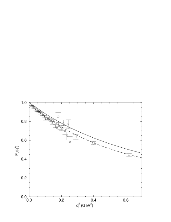
FIG. 1.: Calculated pion form factor compared with data at small $q^{2}$. The data are from Refs. [23] (crosses) and [24] (circles). The solid line is the result obtained when the pseudovector components of the pion Bethe-Salpeter amplitude are included, the dashed-line when they are neglected [14]. On the scale of this figure, both parameter sets in Eq. (57) yield the same calculated result.

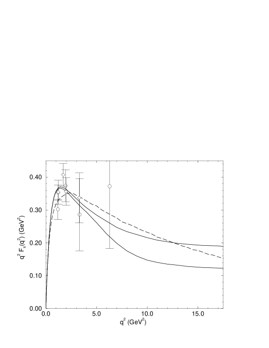
FIG. 2.: Calculated pion form factor compared with the largest $q^{2}$ data available: diamonds - Ref. [24]; and circles - Ref. [25]. The solid lines are the results obtained when the pseudovector components of the pion Bethe-Salpeter amplitude are included (lower line - set A in Eq. (57); upper line - set B), the dashed-line when they are neglected [14].

REFERENCES

• [1] R. B. Wiringa, V. G. J. Stoks and R. Schiavilla, Phys. Rev. C 51, 38 (1995); and references therein.
• [2] A. Bender, C. D. Roberts and L. v. Smekal, Phys. Lett. B 380 (1996) 7; C. D. Roberts, in Quark Confinement and the Hadron Spectrum II, edited by N. Brambilla and G. M. Prosperi (World Scientific, Singapore, 1997), pp. 224-230.
• [3] A. Bashir, A. Kizilersu and M.R. Pennington, Phys. Rev. D 57, 1242 (1998); and references therein.
• [4] C. D. Roberts and A. G. Williams, Prog. Part. Nucl. Phys. 33, 477 (1994).
• [5] P. C. Tandy, Prog. Part. Nucl. Phys. 39, 117 (1997); M. A. Pichowsky and T.-S. H. Lee, Phys. Rev. D 56, 1644 (1997).
• [6] M. A. Ivanov, Yu. L. Kalinovsky, P. Maris and C. D. Roberts, Phys. Rev. C. 57, 1991 (1998); and references therein.
• [7] D. Blaschke, C.D. Roberts and S. Schmidt, β€œThermodynamic properties of a simple, confining model”, nucl-th/9706070, Phys. Lett. B, in press; and references therein.
• [8] Yu. Kalinovsky, K. L. Mitchell and C. D. Roberts, Phys. Lett. B 399, 22 (1997).
• [9] M. B. Hecht, B. H. J. McKellar, β€œDipole moments of the $\rho$-meson”, hep-ph/9704326.
• [10] P. Maris, C. D. Roberts and P. C. Tandy, Phys. Lett. B 420, 267 (1998).
• [11] P. Maris and C. D. Roberts, Phys. Rev. C 56, 3369 (1997).
• [12] R. Delbourgo and M. D. Scadron, J. Phys. G 5, 1621 (1979).
• [13] J. S. Ball and T.-W. Chiu, Phys. Rev. D 22, 2542 (1980).
• [14] C. D. Roberts, Nucl. Phys. A 605, 475 (1996).
• [15] R. Jackiw, β€œField Theoretic Investigations in Current Algebra”, in Current Algebra and Anomalies (World Scientific, Singapore, 1985) pp. 108-141.
• [16] M. Burkardt, M. R. Frank and K. L. Mitchell, Phys. Rev. Lett. 78, 3059 (1997).
• [17] H. Munczek, Phys. Lett. B 175, 215 (1986); C. J. Burden, C. D. Roberts and A. G. Williams, ibid 285, 347 (1992).
• [18] C. D. Roberts, A. G. Williams and G. Krein, Int. J. Mod. Phys. A 4, 1681 (1992).
• [19] D. C. Curtis and M. R. Pennington, Phys. Rev. D 46, 2663 (1992).
• [20] F. T. Hawes, C. D. Roberts and A. G. Williams, Phys. Rev. D 49, 4683 (1994).
• [21] D. B. Leinweber, Ann. Phys. 254, 328 (1997).
• [22] Particle Data Group (R. M. Barnett et al.), Phys. Rev. D 54, 1 (1996).
• [23] S. R. Amendolia, et al., Nucl. Phys. B 277, 168 (1986).
• [24] C. J. Bebek, et al., Phys. Rev. D 13, 25 (1976).
• [25] C. J. Bebek, et al., Phys. Rev. D 17, 1693 (1978).
• [26] G. R. Farrar and D. R. Jackson, Phys. Rev. Lett. 43, 246 (1979).