Power Counting and the Renormalization Group for an Effective Description of $NN$ Scattering

Abstract

I outline the power counting scheme recently introduced by M. Savage, M. Wise and myself for the effective field theory treatment of $NN$ scattering. It is particularly useful for describing systems with a large scattering length, and differs from Weinberg’s power counting. A renormalization group analysis plays a big role in determining the order of a given operator. Pions are ignored in this discussion; how to incorporate them is discussed in M. Savage’s talk [1].

1 Introduction

The purpose of this talk is to outline an effective field theory expansion for $NN$ scattering recently developed in Ref. [2] with my collaborators . When pions are included (Martin Savage’s talk in this volume), this expansion differs from the original approach advocated by Weinberg [3] and implemented or discussed since Refs. [5, 6, 7, 8, 9, 10, 11, 12, 13, 14]. The advantage we claim for our scheme is that it allows analytic calculations of two-nucleon processes in a controlled expansion. As a result, the calculations of low energy $NN$ processes are on the same footing as meson interactions in chiral perturbation theory ($\chi PT$), or meson-baryon interactions in heavy-baryon chiral perturbation theory ($HB\chi PT$). An obvious advantage of this approach is that it is much easier to extract physics from an analytical formula than from a computer simulation; for example, when one computes a Green function in terms of external momenta from Feynman diagrams, on has the whole analytic structure over a wide kinematic range and can analyze inelastic processes by examining the cuts, etc. Furthermore, one can better dissect the result and understand the relative importance from the various contributions. Finally, as we demonstrate explicitly in Ref. [4], by being able to perform analytic calculations one can retire the old spectra of “off-shell ambiguity”, showing it to be hardly worth the fear and loathing that it usually inspires. No $S$-matrix element depends on off-shell quantities!

One might think that in choosing to do an effective field theory calculation of $NN$ interactions analytically rather than numerically, one is sacrificing accuracy for elegance. In fact the power counting suggests this is not the case…Weinberg’s proposal to expand the potential, and then resum its effects to all orders via the Lippmann-Schwinger equation to get the $S$-matrix is not more accurate than simply expanding the $S$-matrix directly. Furthermore, it does not even constitute an expansion unless one chooses the cutoff in the theory with some care. Therefore I see no virtue and some disadvantages with performing an effective field theory expansion of the potential, and then solving the Lippmann-Schwinger equation numerically. I believe that nuclear physics could well profit from abandoning such traditional tools as potentials and wave functions.

Much emphasis has been placed on regulating and renormalizing the effective theory of $NN$ interactions. In fact, I view this workshop as the opportunity to put this issue behind us. The only reason to focus on these issues is to develop a consistent power counting scheme; once such a scheme is developed and followed consistently, results will not be scheme dependent, or else one is working with a model of $NN$ interactions, as opposed to an effective field theory. So, while I emphasize in this talk the renormalization scheme used, the purpose is to develop the tools so that we can do physics, and not out of a love for formalism.

2 Effective field theory for nonrelativistic scattering: a toy example

Consider a toy model of heavy spinless “nucleons” $\tilde{N}$ interacting via a Yukawa interaction characterized by a scale $\Lambda$. For low energy scattering we can construct the effective field theory describing scattering at momenta $p\ll\Lambda$, consisting entirely of contact interactions in a derivative expansion. Since these local operators are singular, the formulation of the low energy theory necessarily introduces divergences that can be dealt with by conventional regularization and renormalization procedures, so that the final result is independent of a momentum cutoff. I will show how to organize the Feynman graphs in the effective theory in a consistent power counting scheme so that the scattering amplitude can be expanded in powers of $p/\Lambda$. Since the sizes of all the coupling constants in the effective theory depend on the subtraction scheme used to render diagrams finite, the development of the power counting scheme is intimately related to the renormalization procedure used. I will explain why the PDS subtraction scheme introduced in Ref. [2] is particularly well suited for this problem.

It should be no surprise that the effective field theory expansion for the toy system is simply related to the conventional effective range expansion, and so the machinery of quantum field theory may appear to be heavy handed and superfluous. Nevertheless, the field theoretic language that I develop in this section is readily extended to the realistic problem of interest: nucleons interacting via both short range interactions and long range pion exchange (see M. Savage’s talk, Ref.[1]). In the realistic problem, effective field theory is not equivalent to an effective range expansion, and is the only framework that can consistently incorporate chiral symmetry and relativistic effects without resorting to phenomenological models.

Assume that the spinless bosons $\tilde{N}$ are nonrelativistic with mass $M$, carry a conserved charge (“baryon number”), and interact via the exchange of a meson $\phi$ with mass $\Lambda$ and coupling $g$. At tree level, meson exchange gives rise to the Yukawa interaction

$$V(r)=-{g^{2}\over 4\pi}{e^{-\Lambda r}\over r},$$ (1)

and the Schrödinger equation for this system may be written as

$$\left[-\nabla_{x}^{2}+\eta{e^{-x}\over x}-{p^{2}\over\Lambda^{2}}\right]\Psi=0\ ,$$ (2)

$$\vec{x}\equiv\Lambda\vec{r},\qquad\eta\equiv{g^{2}M\over 4\pi\Lambda},\qquad p^{2}\equiv ME\ .$$ (3)

Note that $p$ is the magnitude of the 3-momentum carried by each $\tilde{N}$ particle in the center of mass frame. Evidently there are two options for a perturbative solution for the $S$-matrix for this system. The first is an expansion in powers of $\eta$, the familiar Born expansion. An alternative is to expand in powers of $p/\Lambda$, which is the expansion parameter used in effective field theory. An important feature of the low energy expansion is that it can provide accurate results in terms of a few phenomenological parameters even for nonperturbative $\eta$. I will assume throughout that $\eta\sim 1$, since this is the regime we are interested in (a strongly coupled system without a plethora of bound states).

The quantity that is natural to calculate in a field theory is the sum of Feynman graphs, which gives the amplitude $i{\cal A}$, related to the $S$-matrix by

$$S=1+i{Mp\over 2\pi}{\cal A}\ .$$ (4)

For $S$-wave scattering, ${\cal A}$ is related to the phase shift $\delta$ by

$${\cal A}={4\pi\over M}{1\over p\cot\delta-ip}\ .$$ (5)

From quantum mechanics it is well known that it is not ${\cal A}$, but rather the quantity $p\cot\delta$, which has a nice momentum expansion for $p\ll\Lambda$ (the effective range expansion):

$$p\cot\delta=-{1\over a}+{1\over 2}\Lambda^{2}\sum_{n=0}^{\infty}{r}_{n}\left({p^{2}\over\Lambda^{2}}\right)^{n+1}\ ,$$ (6)

where $a$ is the scattering length, and $r_{0}$ is the effective range. So long as $\eta\sim 1$ the coefficients $r_{n}$ are generally $O(1/\Lambda)$ for all $n$. However, $a$ can take on any value, diverging as $\eta$ approaches one of the critical couplings $\eta_{k}$ for which there is a boundstate at threshold. (The lowest critical coupling is found numerically to be $\eta_{1}=1.7$.) Therefore the radius of convergence of a momentum expansion of ${\cal A}$ depends on the size of the scattering length $a$. First I consider the situation where the scattering length is of natural size $|a|\sim 1/\Lambda$, and then I discuss the case $|a|\gg 1/\Lambda$, which is relevant for realistic $NN$ scattering.

2.1 The momentum expansion for a scattering length of natural size

In the regime $|a|\sim 1/\Lambda$ and $|r_{n}|\sim 1/\Lambda$, the amplitude ${\cal A}$ has a simple momentum expansion in terms of the low energy scattering data,

$${\cal A}=-{4\pi a\over M}\left[1-iap+(ar_{0}/2-a^{2})p^{2}+O(p^{3}/\Lambda^{3})\right]\ ,$$ (7)

which converges up to momenta $p\sim\Lambda$. It is this expansion that we wish to reproduce in an effective field theory.

The effective field theory of $\tilde{N}$ particles interacting through contact interactions has the following Lagrangian:

$${\cal L}_{eff} = {{\tilde{N}}^{\dagger}}\left(i\partial_{t}+\nabla^{2}/2M\right)\tilde{N}$$ (8)

$$+(\mu/2)^{4-D}\left[C_{0}({{\tilde{N}}^{\dagger}}\tilde{N})^{2}+{C_{2}\over 8}\left[(\tilde{N}\tilde{N})^{\dagger}(N{\mathop{\nabla}^{\leftrightarrow}}{}^{2}\tilde{N})+h.c\right]+...\right]\ ,$$

where

$${\mathop{\nabla}^{\leftrightarrow}}^{2}\equiv{\mathop{\nabla}^{\leftarrow}}^{2}-2{\mathop{\nabla}^{\leftarrow}\cdot\mathop{\nabla}^{\rightarrow}}+{\mathop{\nabla}^{\rightarrow}}^{2}\ .$$ (9)

The sum of Feynman diagrams computed in this theory gives us the amplitude ${\cal A}$. As I will be using dimensional regularization for the loop integrals in this theory, the spacetime dimension is given by $D$ . The ellipsis indicates higher derivative operators, and $(\mu/2)$ is an arbitrary mass scale introduced to allow the couplings $C_{2n}$ multiplying operators containing $\nabla^{2n}$ to have the same dimension for any $D$. I focus on the $s$-wave channel (generalization to higher partial waves is straightforward), and assume that $M$ is very large so that relativistic effects can be ignored. The form of the $C_{2}$ operator is fixed by Galilean invariance, which implies that when all particle momenta are boosted ${\bf p}\to{\bf p}+M{\bf v}$, the Lagrangian must remain invariant. There exists another two derivative operator for $p$-wave scattering which I will not be discussing.

In general, the tree level $s$ partial wave amplitude in the center of mass frame arising from ${\cal L}_{eff}$ is

$$i{\cal A}_{\rm tree}^{(cm)}=-i(\mu/2)^{4-D}\sum_{n=0}^{\infty}C_{2n}(\mu)p^{2n}\ ,$$ (10)

where the coefficients $C_{2n}(\mu)$ are the couplings in the Lagrangian of operators with $2n$ gradients contributing to $s$-wave scattering. One may always trade time derivatives for spatial gradients, using the equations of motion when computing $S$-matrix elements, and so we ignore such operators (see appendix B in Ref.[4] for an explicit example)..

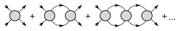
Figure 1: The bubble chain arising from local operators. The vertex is given by the tree level amplitude, eq. (10).

The loop integrals one encounters in diagrams shown in Fig. 1 are of the form

$$\openup 9.0ptI_{n} \equiv i(\mu/2)^{4-D}\int{{\rm d}^{D}q\over(2\pi)^{D}}\,{{\bf q}^{2n}\over\left(E/2+q_{0}-{{\bf q}^{2}\over 2M}+i\epsilon\right)\left(E/2-q_{0}-{{\bf q}^{2}\over 2M}+i\epsilon\right)}$$ (11)

$$= (\mu/2)^{4-D}\int{{{\rm d}}^{(D-1)}{\bf q}\over(2\pi)^{(D-1)}}\,{\bf q}^{2n}\left({1\over E-{\bf q}^{2}/M+i\epsilon}\right)$$

$$= -M(ME)^{n}(-ME-i\epsilon)^{(D-3)/2}\Gamma\left({3-D\over 2}\right){(\mu/2)^{4-D}\over(4\pi)^{(D-1)/2}}\ .$$

In order to define the theory, one must specify a subtraction scheme; different subtraction schemes amount to a reshuffling between contributions from the vertices and contributions from the the UV part of the loop integration. How does one choose a subtraction scheme that is useful? I am considering the case $|a|,|r_{n}|\sim 1/\Lambda$, and wish to reproduce the expansion of the amplitude eq. (7). In order to do this via Feynman diagrams, it is convenient if any Feynman graph with a particular set of operators at the vertices only contributes to the expansion of the amplitude at a particular order. Since the the expansion eq. (7) is a strict Taylor expansion in $p$, it is it is therefore very convenient if each Feynman graph gives one a simple monomial in $p$. Obviously, this won’t be true in a random subtraction scheme. A subtraction scheme that fulfills this criterion is the minimal subtraction scheme ($MS$) which amounts to subtracting any $1/(D-4)$ pole before taking the $D\to 4$ limit. As the integral eq. (11) doesn’t exhibit any such poles, the result in $MS$ is simply

$$I_{n}^{MS}=(ME)^{n}\left({M\over 4\pi}\right)\sqrt{-ME-i\epsilon}=-i\left({M\over 4\pi}\right)p^{2n+1}\ .$$ (12)

Note the nice feature of this scheme that the factors of $q$ inside the loop get converted to factors of $p$, the external momentum. Similarly, a factor of the equations of motion, $i\partial_{t}+\nabla^{2}/2M$, acting on one of the internal legs at the vertex, causes the loop integral to vanish. Therefore one can use the on-shell, tree level amplitude eq. (10) as the internal vertices in loop diagrams; summing the bubble diagrams in the center of mass frame gives

$${\cal A} = -{\sum C_{2n}p^{2n}\over 1+i(Mp/4\pi)\sum C_{2n}p^{2n}}\ .$$ (13)

Since there are no poles at $D=4$ in the $MS$ scheme, the coefficients $C_{2n}$ are independent of the subtraction point $\mu$. The power counting in the $MS$ scheme is particularly simple, as promised:

1. Each propagator counts as $1/p^{2}$;

2. Each loop integration $\int{\rm d}^{4}q$ counts as $p^{5}$ (since $q_{0}\sim{\bf q}^{2}/2M$);

3. Each vertex $C_{2n}\nabla^{2n}$ contributes $p^{2n}$.

The amplitude may be expanded in powers of $p$ as

$${\cal A}=\sum_{n=0}^{\infty}{\cal A}_{n}\ ,\qquad{\cal A}_{n}\sim O(p^{n})$$ (14)

where the ${\cal A}_{n}$ each arise from graphs with $L\leq n$ loops and can be equated to the low energy scattering data eq. (7) in order to fit the $C_{2n}$ couplings. In particular, ${\cal A}_{0}$ arises from the tree graph with $C_{0}$ at the vertex; ${\cal A}_{1}$ is given by the 1-loop diagram with two $C_{0}$ vertices; ${\cal A}_{2}$ is gets contributions from both the 2-loop diagram with three $C_{0}$ vertices, as well as the tree diagram with one $C_{2}$ vertex, and so forth. Thus the first three terms are

$${\cal A}_{0}=-C_{0}\ ,\qquad{\cal A}_{1}=iC_{0}^{2}{Mp\over 4\pi}\ ,\qquad{\cal A}_{2}=C_{0}^{3}\left({Mp\over 4\pi}\right)^{2}-C_{2}p^{2}\ .$$ (15)

Comparing eqs. (7, 15) I find for the first two couplings of the effective theory

$$C_{0}={4\pi a\over M}\ ,\qquad C_{2}=C_{0}{ar_{0}\over 2}\ .$$ (16)

In general, when the scattering length has natural size,

$$C_{2n}\sim{4\pi\over M\Lambda}{1\over\Lambda^{2n}}\ .$$ (17)

Note that the effective field theory calculation in this scheme is completely perturbative even though $\eta\sim 1$ and there may be a boundstate well below threshold. The point is, that when there are no poles in ${\cal A}$ in the region $|p|\ \raise 1.29167pt\hbox{$<$\kern-7.5pt\lower 4.30554pt\hbox{$\sim$}}\ \Lambda$, the amplitude is amenable to a Taylor expansion in $p/\Lambda$ in that region; with a suitable subtraction scheme ($MS$), this Taylor expansion can correspond to a perturbative sum of Feynman graphs.

2.2 The momentum expansion for large scattering length

Now consider the case $|a|\gg 1/\Lambda$, $|r_{n}|\sim 1/\Lambda$, which is of relevance to realistic $NN$ scattering. For a nonperturbative interaction ($\eta\sim 1$) with a boundstate near threshold, the expansion of ${\cal A}$ in powers of $p$ is of little practical value, as it breaks down for momenta $p\ \raise 1.29167pt\hbox{$>$\kern-7.5pt\lower 4.30554pt\hbox{$\sim$}}\ 1/|a|$, far below $\Lambda$. In the above effective theory, this occurs because the couplings $C_{2n}$ are anomalously large, $C_{2n}\sim 4\pi a^{n+1}/M\Lambda^{n}$. However, the problem is not with the effective field theory method, but rather with the subtraction scheme chosen.

Instead of reproducing the expansion of the amplitude shown in eq. (7), one needs to expand in powers of $p/\Lambda$ while retaining $ap$ to all orders:

$${\cal A}=-{4\pi\over M}{1\over(1/a+ip)}\left[1+{r_{0}/2\over(1/a+ip)}p^{2}+{(r_{0}/2)^{2}\over(1/a+ip)^{2}}p^{4}+{(r_{1}/2\Lambda^{2})\over(1/a+ip)}p^{4}+\ldots\right]$$ (18)

Note that for $p>1/|a|$ the terms in this expansion scale as $\{p^{-1},p^{0},p^{1},\ldots\}$. Therefore, the expansion in the effective theory should take the form

$${\cal A}=\sum_{n=-1}^{\infty}{\cal A}_{n}\ ,\qquad{\cal A}_{n}\sim O(p^{n})$$ (19)

beginning at $n=-1$ instead of $n=0$, as in the expansion eq. (14). Comparing with eq. (18), we see that

$${\cal A}_{-1} = -{4\pi\over M}{1\over(1/a+ip)}\ ,$$

$${\cal A}_{0} = -{4\pi\over M}{r_{0}p^{2}/2\over(1/a+ip)^{2}}\ ,$$ (20)

and so forth. Again, the task is to compute the ${\cal A}_{n}$ in the effective theory, and equate to the appropriate expression above, thereby fixing the $C_{2n}$ coefficients. As before, the goal is actually more ambitious: each particular graph contributing to ${\cal A}_{n}$ should be $O(p^{n})$, so that the power counting is transparent.

As any single diagram in the effective theory is proportional to positive powers of $p$, computing the leading term ${\cal A}_{-1}$ must involve summing an infinite set of diagrams. It is easy to see that the leading term ${\cal A}_{-1}$ can be reproduced by the sum of bubble diagrams with $C_{0}$ vertices [3], which yields in the $MS$ scheme

$${\cal A}_{-1}={-C_{0}\over\left[1+{C_{0}M\over 4\pi}ip\right]}\ .$$ (21)

Comparing this with eq. (20) gives $C_{0}=4\pi a/M$, as in the previous section. However, there is no expansion parameter that justifies this summation: each individual graph in the bubble sum goes as $C_{0}(C_{0}Mp)^{L}\sim(4\pi a/M)(iap)^{L}$, where $L$ is the number of loops. Therefore each graph in the bubble sum is bigger than the preceding one, for $|ap|>1$, while they sum up to something small.

This is an unpleasant situation for an effective field theory; it is important to have an expansion parameter so that one can identify the order of any particular graph, and sum the graphs consistently. Without such an expansion parameter, one cannot determine the size of omitted contributions, and one can end up retaining certain graphs while dropping operators needed to renormalize those graphs. This results in a model-dependent description of the short distance physics, as opposed to a proper effective field theory calculation.

Since the sizes of the contact interactions depend on the renormalization scheme one uses, the task becomes one of identifying the appropriate subtraction scheme that makes the power counting simple and manifest. The $MS$ scheme fails on this point; however this is not a problem with dimensional regularization, but rather a problem with the minimal subtraction scheme itself. The momentum space subtraction at threshold used in Ref. [3] behaves similarly.

Next, consider an alternative regularization and renormalization scheme, namely to using a momentum cutoff equal to $\Lambda$. Then for large $a$ one finds $C_{0}\sim(4\pi/M\Lambda)$, and each additional loop contributes a factor of $C_{0}(\Lambda+ip)M/4\pi\sim(1+ip/\Lambda)$. The problem with this scheme is that for $\Lambda\gg p$ the term $ip/\Lambda$ from the loop is small relative to the $1$, and ought to be ignorable; however, neglecting it would fail to reproduce the desired result eq. (20). This scheme suffers from significant cancellations between terms, and so once again the power counting is not manifest.

Evidently, since ${\cal A}_{-1}$ scales as $1/p$, the desired expansion would have each individual graph contributing to ${\cal A}_{-1}$ scale as $1/p$. As the tree level contribution is $C_{0}$, I must therefore have $C_{0}$ be of size $\propto 1/p$, and each additional loop must be $O(1)$. This can be achieved by using dimensional regularization and the PDS (power divergence subtraction) scheme introduced in Ref. [2]. The PDS scheme involves subtracting from the dimensionally regulated loop integrals not only the $1/(D-4)$ poles corresponding to log divergences, as in $MS$, but also poles in lower dimension which correspond to power law divergences at $D=4$. The integral $I_{n}$ in eq. (11) has a pole in $D=3$ dimensions which can be removed by adding to $I_{n}$ the counterterm

$$\delta I_{n}=-{M(ME)^{n}\mu\over 4\pi(D-3)},$$ (22)

so that the subtracted integral in $D=4$ dimensions is

$$I_{n}^{PDS}=I_{n}+\delta I_{n}=-(ME)^{n}\left({M\over 4\pi}\right)(\mu+ip).$$ (23)

In this subtraction scheme

$${\cal A} = -{M\over 4\pi}\left[{4\pi\over M\sum C_{2n}p^{2n}}+\mu+ip\right]^{-1}\ .$$ (24)

By performing a Taylor expansion of the denominator of the above expression, and comparing with eq. (18), one finds that for $\mu\gg 1/|a|$, the couplings $C_{2n}(\mu)$ scale as

$$C_{2n}(\mu)\sim{4\pi\over M\Lambda^{n}\mu^{n+1}}\ .$$ (25)

Eq. 25 implies that $\mu\sim p$, $C_{2n}(\mu)\sim 1/p^{n+1}$. A factor of $\nabla^{2n}$ at a vertex scales as $p^{2n}$, while each loop contributes a factor of $p$. The power counting rules for the case of large scattering length are therefore:

1. Each propagator counts as $1/p^{2}$;

2. Each loop integration $\int{\rm d}^{4}q$ counts as $p^{5}$;

3. Each vertex $C_{2n}\nabla^{2n}$ contributes $p^{n-1}$.

We see that this scheme avoids the problems encountered with the choices of the $MS$ ($\mu=0$) or momentum cuttoff ($\mu\sim\Lambda$) schemes. First of all, a tree level diagram with a $C_{0}$ vertex is $O(p^{-1})$, while each loop with a $C_{0}$ vertex contributes $C_{0}(\mu)M(\mu+ip)/4\pi\sim 1$. Therefore each term in the bubble sum contributing to ${\cal A}_{-1}$ is of order $p^{-1}$, unlike the case for $\mu=0$. Secondly, since $\mu\sim p$, it makes sense keeping both the $\mu$ and the $ip$ in eq. (23) as they are of similar size, unlike what we found in the $\mu=\Lambda$ case. The PDS scheme retains the nice feature of $MS$ that powers of $q$ inside the loop integration are effectively replaced by powers of the external momentum $p$ .

Starting from the above counting rules one finds that the leading order contribution to the scattering amplitude ${\cal A}_{-1}$ scales as $p^{-1}$ and consists of the sum of bubble diagrams with $C_{0}$ vertices; contributions to the amplitude scaling as higher powers of $p$ come from perturbative insertions of derivative interactions, dressed to all orders by $C_{0}$. The first three terms in the expansion are

$${\cal A}_{-1} = {-C_{0}\over\left[1+{C_{0}M\over 4\pi}(\mu+ip)\right]}\ ,$$

$${\cal A}_{0} = {-C_{2}p^{2}\over\left[1+{C_{0}M\over 4\pi}(\mu+ip)\right]^{2}}\ ,$$

$${\cal A}_{1} = \left({(C_{2}p^{2})^{2}M(\mu+ip)/4\pi\over\left[1+{C_{0}M\over 4\pi}(\mu+ip)\right]^{3}}-{C_{4}p^{4}\over\left[1+{C_{0}M\over 4\pi}(\mu+ip)\right]^{2}}\right)\ ,$$ (26)

where the first two correspond to the Feynman diagrams in Fig. 2. The third term, ${\cal A}_{1}$, comes from graphs with either one insertion of $C_{4}\nabla^{4}$ or two insertions of $C_{2}\nabla^{2}$, dressed to all orders by the $C_{0}$ interaction.

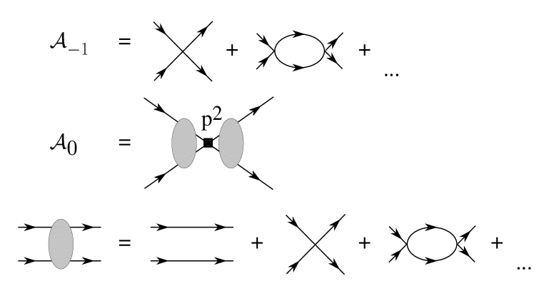
Figure 2: Leading and subleading contributions arising from local operators.

Comparing eq. (26) with the expansion of the amplitude eq. (18), the couplings $C_{2n}$ are related to the low energy scattering data $a$, $r_{n}$:

$$C_{0}(\mu) = {4\pi\over M}\left({1\over-\mu+1/a}\right)\ ,$$

$$C_{2}(\mu) = {4\pi\over M}\left({1\over-\mu+1/a}\right)^{2}{{r}_{0}\over 2}\ ,$$

$$C_{4}(\mu) = {4\pi\over M}\left({1\over-\mu+1/a}\right)^{3}\left[{1\over 4}{r}_{0}^{2}+{1\over 2}{{r}_{1}\over\Lambda^{2}}\left({-\mu+1/a}\right)\right]\ .$$ (27)

Note that assuming $r_{n}\sim 1/\Lambda$, these expressions are consistent with the scaling law in eq. (25).

2.3 The renormalization group

This power counting described in the previous section relies entirely on the running of $C_{2n}(\mu)$ as a function of $\mu$ given in eq. (25). This was derived by summing up all of the diagrams in Fig. 1 explicitly, and then comparing with the form of a general amplitude, eq. (5). When pions are included in real $NN$ interactions, the diagrams in Fig. 1 cannot be explicitly summed. However, the power counting can be established perturbatively by examining the $\beta$-functions and the renormalization group running of the $C_{2n}(\mu)$ couplings. The dependence of $C_{2n}(\mu)$ on $\mu$ is determined by the requirement that the amplitude be independent of the arbitrary parameter $\mu$. The physical parameters $a$, $r_{n}$ enter as boundary conditions on the RG equations.

The $\beta$-function $\beta_{2n}$ for the coupling $C_{2n}$ is defined by

$$\beta_{2n}\equiv\mu{{\rm d}C_{2n}\over{\rm d}\mu}\ ,$$ (28)

and all of the $\beta$-functions can be computed by requiring that any physical quantity (e.g. the scattering amplitude) be independent of $\mu$. In the PDS scheme, the $\mu$ dependence of the $C_{2n}$ coefficients enters either logarithmically or linearly, associated with simple $1/(D-4)$ or $1/(D-3)$ poles respectively. The functions $\beta_{2n}$ follow straightforwardly from $\mu{d\over d\mu}(1/{\cal A})=0$, using the expression for ${\cal A}$ in eq. (24). This gives

$$\beta_{2n}={M\mu\over 4\pi}\sum_{m=0}^{n}C_{2m}C_{2(n-m)}\ .$$ (29)

Figure 3: Graphs contributing to the $\beta$-functions for $C_{2n}$

However, I did not need the full, explicit amplitude ${\cal A}$ to compute $\beta_{2n}$, as the exact $\beta$-functions can be computed from the one-loop diagrams shown in Fig. 3. That is because only the one-loop diagrams contribute to simple poles. Without pions, the only poles one encounters are all of the form $1/(D-3)$.

We examine the RG equations for the first two couplings, $C_{0}$ and $C_{2}$, in order to explicitly show how one recovers the results in eq. (27) from solving the renormalization group equations. From eq. (29)—or equivalently, the diagrams in Fig. 3— it follows that

$$\beta_{0} = {M\mu\over 4\pi}C_{0}^{2}\ ,$$

$$\beta_{2} = 2{M\mu\over 4\pi}C_{0}C_{2}\ .$$ (30)

Integrating these equations relates the $C_{2n}$ coefficients at two different renormalization scales $\mu$ and $\mu_{0}$. Comparing the theory with ${\cal A}$ and its derivatives at $\mu=p=0$ determines the initial values $C_{2n}(0)$ as in eq. (16). The solutions to eq. (30) are

$$C_{0}(\mu) = {C_{0}(\mu_{0})\over 1+C_{0}(\mu_{0})M(\mu_{0}-\mu)/4\pi}\ ,$$

$$C_{2}(\mu) = C_{2}(\mu_{0})\left({C_{0}(\mu)\over C_{0}(\mu_{0})}\right)^{2}\ .$$ (31)

The boundary conditions are supplied by equating the computed ${\cal A}$ to scattering data at $\mu=p=0$ , which yields

$$C_{0}(0) = 4\pi a/M\ ,\qquad C_{2}(0)=C_{0}(0)ar_{0}/2\ ,$$ (32)

and so forth. With these boundary conditions and the solutions eq. (31) we arrive at the result derived previously for $C_{0}(\mu)$ and $C_{2}(\mu)$ in eq. (27):

$$C_{0}(\mu)={4\pi\over M}\left({1\over-\mu+1/a}\right)\ ,$$

$$C_{2}(\mu)={4\pi\over M}\left({1\over-\mu+1/a}\right)^{2}{{r}_{0}\over 2}\ .$$ (33)

It is instructive to solve the complete, coupled RG equation

$$\mu{{\rm d}\ \over{\rm d}\mu}C_{2n}={M\mu\over 4\pi}\sum_{m=0}^{n}C_{2m}C_{2(n-m)}$$ (34)

for the leading small $\mu$ behavior of each of the coefficients $C_{2n}$ . The solution, for $n>0$ is

$$C_{2n}(\mu)={4\pi\over M(-\mu+1/a)}\left({r_{0}/2\over-\mu+1/a}\right)^{n}+O(\mu^{-n})\ .$$ (35)

First note that the scaling property in eq. (25) is realized: $C_{2n}(\mu)\propto\mu^{-(n+1)}$ for $|1/a|\ll\mu\ll\Lambda$. What is curious is that this leading behavior does not entail a new integration constant for each $n$, but only depends on the two parameters $a$ and $r_{0}$ encountered when solving for $C_{0}(\mu)$ and $C_{2}(\mu)$; this is due to a quasi-fixed point behavior of the RG equations — the $C_{2n}$ couplings are being driven primarily by lower dimensional interactions. One can see this explicitly in our formula eq. (27) for $C_{4}$, where the leading $O(\mu^{-3})$ part of $C_{4}$ depends only on $r_{0}$, while the subleading $O(\mu^{-2})$ part is proportional to $r_{1}$.

This behavior allows us to establish a connection between the present work, and the method of introducing an $s$-channel dibaryon discussed in Ref. [16]. The leading $\mu$ behavior of all of the $C_{2n}$ coefficients is determined by the effective range $r_{0}$. If one resums this leading behavior at the $\tilde{N}\tilde{N}$ vertex one finds (for $\mu\sim p\gg 1/|a|$)

$$\sum_{n=0}^{\infty}C_{2n}(\mu)p^{2n} = {4\pi\over M}{1\over-\mu+1/a-{r_{0}p^{2}\over 2}}+O(p^{2})$$ (36)

$$= -{(8\pi/M^{2}r_{0})\over E-(-\mu+1/a)/Mr_{0}}\ .$$

This looks like an $s$-channel propagator for a particle at rest of mass $[2M+(-\mu+1/a)/Mr_{0}]$, and in fact, for $\mu=0$, corresponds exactly to the dibaryon proposed in Ref. [16] to reproduce the scattering due to a short range potential. We see that using the dibaryon is as good as (but no better than) carrying out the effective field theory calculation to $O(p^{1})$. The subleading corrections can be accounted for by including the subleading part of the $C_{4}(\mu)p^{4}$ vertex proportional to $r_{1}$, and which occurs at $O(p^{2})$. This dibaryon was recently used with great success in the three-body problem [17].

3 Expanding the potential or the scattering amplitude?

Throughout this talk I have discussed an expansion of the scattering amplitude, while most previous work in the subject of effective field theory for $NN$ scattering has emphasized expansion of the potential[3, 5, 6, 7, 8, 9, 10, 11, 12, 13, 14], followed by a solution of the Lippmann-Schwinger equation with this approximate potential. Since every observable is an $S$-matrix element, it would seem that the two methods, if carried out to the same order, ought to give answers that disagree only by higher order effects. For example, if working to $O(p^{0})$, the direct expansion of ${\cal A}\simeq{\cal A}_{-1}+{\cal A}_{0}$ is linear in the $C_{2}\nabla^{2}$ operator. Alternatively, if the potential is expanded to linear order in $C_{2}\nabla^{2}$, the Lippmann-Schwinger equation yields an amplitude which reproduces the term linear in $C_{2}$, but also includes terms higher order in $C_{2}$. These terms nonlinear in $C_{2}$ would appear to be higher order effects and negligible.

This is not in general true, however. Unlike the ${\cal A}$ expansion I have outlined which is explicitly scheme independent, the Lippmann-Schwinger approach is not. That is because the time ordered product of several insertions of the potential induces new divergences that require counterterms not included in the expansion. For example, when the potential is taken to include only the $C_{0}$ and $C_{2}\nabla^{2}$ operators, the one-loop contribution to the Lippmann-Schwinger equation has a divergence that requires the $C_{4}\nabla^{4}$ operator to absorb the divergence—an operator not included in the expansion! As a result, the Lippmann-Schwinger approach is necessarily scheme-dependent.

Is this bad? Not fatal, but undesirable. It means that the size of neglected effects depends on the renormalization scheme and cutoff or renormalization scale. That is why in calculations of this sort, the renormalization scale or cutoff becomes an extra parameter that has to be chosen to minimize the errors.

Understanding the scheme dependence of the Lippmann-Schwinger result helps explain an apparent paradox: the amplitude ${\cal A}$ calculated in this talk in the ${\it PDS}\$ scheme is $\mu$ independent at each order in the expansion. In particular, each term ${\cal A}_{n}$ is unchanged if I take $\mu\to 0$, which is the $MS$ scheme. However, there have been numerous discussions about how $MS$ is sick. In fact, $MS$ is not sick except for the fact that at any given order there tend to be large cancellations among the graphs included at that order. However, in the Lippmann-Schwinger approach, parts of higher order terms are kept, which destroys the cancellations; the result is $\mu$ dependent, and the expansion becomes very bad for $\mu\ll p$. For example, at $O(p^{1})$, ${\cal A}_{1}$ given in eq. (26) involves both a $C_{2}^{2}$ term and a $C_{4}$ term; for $\mu\ll p$ these two terms are both large and cancel against each other. However the $O(p^{0})$ Lippmann-Schwinger calculation, in which the potential includes the $C_{2}$ interaction, but not the $C_{4}$ term, gives a scattering amplitude that includes the $C_{2}^{2}$ piece of ${\cal A}_{1}$ but not the $C_{4}$ piece which is needed to largely cancel the $C_{2}^{2}$ contribution and render its effects small. If one solves the Lippmann-Schwinger equation and chooses the ${\it PDS}\$ value $\mu\sim p$, then the $C_{2}^{2}$ and $C_{4}$ terms in ${\cal A}_{1}$ are of the same size and (by construction) and small, and the error in the Lippmann-Schwinger amplitude really is higher order. This has been independently discussed in Ref. [13].

The correct statement about the $MS$ subtraction scheme is that it can be misleading, in that one cannot look at an individual Feynman graph at contributing to ${\cal A}_{n}$ and expect it to contribute at $O(p^{n})$. The problems with the $MS$ scheme reported in the literature [7, 9, 10, 14] are the result of combining the $MS$ scheme with the scheme dependent Lippmann-Schwinger approach. I favor avoiding the Lippmann-Schwinger approach altogether—why would one want a calculational scheme where the size of the errors at a given order in the expansion depend on the renormalization scheme? In effective field theory, with its necessarily singular interactions that require renormalization, the concept of a classical potential does not seem very useful.

4 Conclusions and a challenge

I hope I have convinced you that there exists a rather simple and well defined approach to calculating low energy processes involving two nucleons. There are quite a few interactions of interest to calculate, such as $NN\to NN\gamma$, $NN\to d\gamma$, $pp\to de^{+}\nu$, $\pi d\to\pi d$, as well as isospin violation and parity violation in $NN$ scattering. And for every calculation, there is always one higher order that can be computed!

However, it would be disappointing if the applicability of these techniques were limited to two nucleon processes. Evidence to date [2, 4] suggests that the expansion works reasonably well up to momenta comparable to the Fermi momentum in nuclear matter. What are the prospects of using effective field theory to discuss the structure of nuclei, or the equation of state of nuclear matter?

At present the road block is the three-body interaction. It is tempting to dismiss the three-body interaction as negligible, as often claimed. However, the two-body interactions renormalize the three-body force, which means that in fact the strength of the three-body interaction is scheme dependent, and saying it is small in general is nonsensical. In fact, because of the Efimov [18] and Thomas [19] effects, we know that we cannot keep zero-range two-body interactions while neglecting three-body interactions. It is clear, due to Pauli statistics, that at most there can be four-body contact interactions (without derivatives). However, until the properties of the three- and four- body interactions are understood properly, it is unclear how to proceed to a discussion of nuclear matter. I view understanding this issue of few-body interactions to be the fundamental challenge in this field.

References

References

- [1] M. J. Savage, Including Pions, nucl-th/9804034.
- [2] D.B. Kaplan, M.J. Savage and M.B. Wise, nucl-th/9801034, to appear in Phys. Lett. B; nucl-th/9802075, submitted to Nucl. Phys. B.
- [3] S. Weinberg, Phys. Lett. B251 (1990) 288; Nucl. Phys. B363 (1991) 3; Phys. Lett. B295 (1992) 114.
- [4] D. B. Kaplan, M. J. Savage, M. B. Wise, nucl-th/9804032, submitted to Nucl. Phys. B
- [5] C. Ordonez and U. van Kolck, Phys. Lett. B291 (1992) 459; C. Ordonez, L. Ray and U. van Kolck, Phys. Rev. Lett. 72 (1994) 1982; Phys. Rev. C53 (1996) 2086.; U. van Kolck, Phys. Rev. C49 (1994) 2932.
- [6] T.-S. Park, D-.P. Min and M. Rho, Phys. Rev. Lett. 74 (1995) 4153; Nucl. Phys. A596 (1996) 515; T.-S. Park, K. Kubodera, D.-P. Min, M. Rho, hep-ph/9711463.
- [7] D.B. Kaplan, M.J. Savage and M.B. Wise, Nucl. Phys. B 478, 629 (1996), nucl-th/9605002.
- [8] T. Cohen, J.L. Friar, G.A. Miller and U. van Kolck, Phys. Rev. C 53, 2661 (1996).
- [9] T.D. Cohen, Phys. Rev. C 55, 67 (1997). D.R. Phillips and T.D. Cohen, Phys. Lett. B 390, 7 (1997). K.A. Scaldeferri, D.R. Phillips, C.W. Kao and T.D. Cohen, Phys. Rev. C 56, 679 (1997). S.R. Beane, T.D. Cohen and D.R. Phillips, nucl-th/9709062.
- [10] G. P. Lepage, How to renormalize the Schrödinger Equation, Lectures given at 9th Jorge Andre Swieca Summer School: Particles and Fields, Sao Paulo, Brazil, 16-28 Feb 1997. nucl-th/9706029.
- [11] S.K. Adhikari and A. Ghosh, J. Phys. A30, 6553 (1997).
- [12] K.G. Richardson, M.C. Birse and J.A. McGovern, hep-ph/9708435.
- [13] J. Gegelia, nucl-th/9802038.
- [14] J.V. Steele and R.J. Furnstahl, nucl-th/9802069.
- [15] A.V. Manohar, Lectures given at 35th Internationale Universitatswochen für Kern- und Teilchenphysik, Perturbative and Nonperturbative Aspects of Quantum Field Theory, Schladming, Austria, 2-9 Mar 1996. hep-ph/9606222 .
- [16] D. B. Kaplan, Nucl. Phys. B 494 (1997) 471, nucl-th/9610052.
- [17] P.F. Bedaque and U. van Kolck, nucl-th/9710073; P.F. Bedaque, H.-W. Hammer and U. van Kolck, nucl-th/9802057.
- [18] V. N. Efimov, Sov. Jour. of Nucl. Phys. 12 (1971) 589.
- [19] L. H. Thomas, Phys. Rev. 47 (1935) 903.