Relativistic and Non-Relativistic Mean Field Investigation of the Superdeformed Bands in ⁶²Zn

Abstract

Following the discovery of the superdeformed(SD) band in ⁶²Zn, we calculate several low-lying SD bands in ⁶²Zn using Relativistic Mean Field and Skyrme-Hartree-Fock models. Both models predict similar results, but still we can see some qualitative differences in the results of these two models, which are coming from the difference of the detail of single-particle levels.

and

Recent development of the experimental techniques enables us to study the nuclei at very high angular momentum. The study of the superdeformed(SD) bands is one of the most interesting topics in such studies. The first experimental discovery was done for ¹⁵²Dy in 1986[1]. Since then, a large number of the SD bands have been observed in the $A\sim$150, 130, 190 and 80 mass regions. These SD states are generated on the second minima in the potential energy surface which are connected with the deformed shell gaps such as $N,Z\sim$44, 64, 86 and 116. Based on the theoretical calculation indicating that there exist the $N,Z\sim$30 shell gaps, the SD bands in the $A\sim$60 mass region were also predicted[2]. In spite of much experimental effort, however, such SD states had not been observed due to some experimental difficulties. In 1997, a cascade of six $\gamma$ rays forming a new band was observed in ⁶²Zn[3], which was the first experimental discovery of the SD bands in this mass region. The extracted $\beta_{2}$ value is 0.45${}^{+0.10}_{-0.07}$, and the SD states seem to become yrast at $I\mathrel{\mathchoice{\lower 2.58334pt\vbox{\halign{$\m@th\displaystyle\hfil#\hfil$\cr>\crcr\sim\crcr}}}{\lower 2.58334pt\vbox{\halign{$\m@th\textstyle\hfil#\hfil$\cr>\crcr\sim\crcr}}}{\lower 2.58334pt\vbox{\halign{$\m@th\scriptstyle\hfil#\hfil$\cr>\crcr\sim\crcr}}}{\lower 2.58334pt\vbox{\halign{$\m@th\scriptscriptstyle\hfil#\hfil$\cr>\crcr\sim\crcr}}}}$24 in comparison with a theoretical calculation[3]. This spin value corresponds to the rotational frequency $\Omega\mathrel{\mathchoice{\lower 2.58334pt\vbox{\halign{$\m@th\displaystyle\hfil#\hfil$\cr>\crcr\sim\crcr}}}{\lower 2.58334pt\vbox{\halign{$\m@th\textstyle\hfil#\hfil$\cr>\crcr\sim\crcr}}}{\lower 2.58334pt\vbox{\halign{$\m@th\scriptstyle\hfil#\hfil$\cr>\crcr\sim\crcr}}}{\lower 2.58334pt\vbox{\halign{$\m@th\scriptscriptstyle\hfil#\hfil$\cr>\crcr\sim\crcr}}}}$1.3 MeV which is the highest frequency among those observed so far. Besides, there are several interesting features in this mass region, for example, that the valence neutrons and protons occupy the same orbits in contrast with those in other mass regions and the residual neutron-proton pairing at high spin may be observed. Another example is the decay of these SD shapes via proton emission due to a very low Coulomb barrier. Such decay of the well-deformed high spin states has been already observed in ⁵⁸Cu[4]. For this $A\sim$60 mass region, more and more new experimental data will become available in near future and so many theoretical investigations will be done from now on, using both the semi-phenomenological models such as cranked Nilsson (or Woods-Saxon)-Strutinski model and fully microscopic ones, for example, cranked Hartree-Fock model with density dependent effective interactions and Relativistic Mean Field(RMF) model.

RMF model is now considered as a reliable method likely to the non-relativistic Hartree-Fock model to describe various properties of finite nuclei, not only $\beta$-stable but also $\beta$-unstable ones. Since the work of Walecka and his collaborators[5, 6, 7], RMF model has been applied to nuclear matter and the ground states of finite nuclei as well as the scattering data with great successes. Some groups also tried to apply this model to the excited states in finite nuclei. In 1989, Munich group made a first attempt to describe the properties of rotating nuclei[8, 9]. They applied this model mainly to the SD bands in the $A\sim$150, 80 and 190 mass regions [10, 11, 12, 13]. The RMF calculations of rotating nuclei are, however, limited to the nuclei in these mass regions up to now. Because RMF model is on its way of refinement, it is surely important to apply this model to various nuclear phenomena as wide as possible, and to check its applicability further. Therefore, in this letter, we apply RMF model to the description of the SD bands in ⁶²Zn including the newly discovered one, and examine how well this model can describe the very high spin states in neutron-deficient unstable nuclei. This is the first RMF calculation of the SD bands in this mass region. For comparison, we also calculate the SD bands in ⁶²Zn using Skyrme-Hartree-Fock(SHF) model.

The starting point of RMF model is the following Lagrangian which contains the nucleon and several kinds of meson fields such as $\sigma$-, $\omega$- and $\rho$-mesons, together with the photon fields(denoted by $A$) mediating the Coulomb interaction,

$${\cal L}={\cal L}_{N}+{\cal L}_{\sigma}+{\cal L}_{\omega}+{\cal L}_{\rho}+{\cal L}_{A}+{\cal L}_{\rm int}+{\cal L}_{\rm NL},$$

$${\cal L}_{N} = \overline{\psi}(i\gamma^{\alpha}\partial_{\alpha}-M)\psi,$$

$${\cal L}_{\sigma} = \frac{1}{2}(\partial_{\alpha}\sigma)(\partial^{\alpha}\sigma)-\frac{1}{2}m_{\sigma}^{2}\sigma^{2},$$

$${\cal L}_{\omega} = -\frac{1}{4}\Omega_{\alpha\beta}\Omega^{\alpha\beta}+\frac{1}{2}m_{\omega}^{2}\omega_{\alpha}\omega^{\alpha},$$

$${\cal L}_{\rho} = -\frac{1}{4}\mbox{\boldmath$R$}_{\alpha\beta}\cdot\mbox{\boldmath$R$}^{\alpha\beta}+\frac{1}{2}m_{\rho}^{2}\mbox{\boldmath$\rho$}_{\alpha}\cdot\mbox{\boldmath$\rho$}^{\alpha},$$

$${\cal L}_{A} = -\frac{1}{4}F_{\alpha\beta}F^{\alpha\beta},$$

where

$$\Omega_{\alpha\beta} = \partial_{\alpha}\omega_{\beta}-\partial_{\beta}\omega_{\alpha},$$

$$\mbox{\boldmath$R$}_{\alpha\beta} = \partial_{\alpha}\mbox{\boldmath$\rho$}_{\beta}-\partial_{\beta}\mbox{\boldmath$\rho$}_{\alpha}-g_{\rho}\mbox{\boldmath$\rho$}_{\alpha}\times\mbox{\boldmath$\rho$}_{\beta},$$

$$F_{\alpha\beta} = \partial_{\alpha}A_{\beta}-\partial_{\beta}A_{\alpha},$$

are the field strength tensors. ${\cal L}_{\rm int}$ is the interaction part between nucleons and mesons,

$$\begin{array}[]{ccl}{\cal L}_{\rm int}&=&g_{\sigma}\overline{\psi}\psi\sigma-g_{\omega}\overline{\psi}\gamma^{\alpha}\psi\omega_{\alpha}\\ &&-g_{\rho}\overline{\psi}\gamma^{\alpha}\mbox{\boldmath$\tau$}\psi\cdot\mbox{\boldmath$\rho$}_{\alpha}-e\overline{\psi}\gamma^{\alpha}\frac{\displaystyle 1-\tau_{3}}{\displaystyle 2}\psi A_{\alpha}.\end{array}$$

In the standard applications, the non-linear self interactions among the $\sigma$-mesons,

$${\cal L}_{\rm NL}=\frac{1}{3}g_{2}\sigma^{3}-\frac{1}{4}g_{3}\sigma^{4},$$

are also included, which are crucial for the realistic description of deformed nuclei. Applying the variational principle to the Lagrangian gives the equations of motion. Within the mean field approximation, these are the Dirac equation for single nucleon fields $\psi_{i}$ and the Klein-Gordon equations for the classical meson and photon fields. After solving these equations, we can calculate various properties of finite nuclei.

For the application to rotating nuclei within the cranking assumption, it is necessary at first to write the Lagrangian in the uniformly rotating frame which rotates around the $x$-axis with a constant angular velocity $\Omega$, from which the equations of motion in this rotating frame can be obtained. Because the rotating frame is not an inertial one, a fully covariant formulation is desirable and we accomplished this using the technique of general relativity known as tetrad formalism[14, 15]. The procedure is as follows: First, according to tetrad formalism, we can write the Lagrangian in the non-inertial frame represented by the metric tensor $g_{\mu\nu}(x)$. Then the variational principle gives the equations of motion in this non-inertial frame. Finally, substituting the metric tensor of the uniformly rotating frame,

$$g_{\mu\nu}(x)=\left(\begin{array}[]{cccc}1-\Omega^{2}(y^{2}+z^{2})&0&\Omega z&-\Omega y\\ 0&-1&0&0\\ \Omega z&0&-1&0\\ -\Omega y&0&0&-1\end{array}\right),$$

leads to the desired equations of motion. The resulting equations are

$$\left\{\mbox{\boldmath$\alpha$}\cdot(\frac{1}{i}\mbox{\boldmath$\nabla$}-g_{\omega}\mbox{\boldmath$\omega$}(x))+\beta(M-g_{\sigma}\sigma(x))\right.$$

$$\left.+g_{\omega}\omega^{0}(x)-\Omega(L_{x}+\Sigma_{x})\right\}\psi_{i}(x) = \epsilon_{i}\psi_{i}(x),$$

$$\left\{-\mbox{\boldmath$\nabla$}^{2}+m_{\sigma}^{2}-\Omega^{2}L_{x}^{2}\right\}\sigma(x) = g_{\sigma}\rho_{s}(x),$$

$$\left\{-\mbox{\boldmath$\nabla$}^{2}+m_{\omega}^{2}-\Omega^{2}L_{x}^{2}\right\}\omega^{0}(x) = g_{\omega}\rho_{v}(x),$$

$$\left\{-\mbox{\boldmath$\nabla$}^{2}+m_{\omega}^{2}-\Omega^{2}(L_{x}+S_{x})^{2}\right\}\mbox{\boldmath$\omega$}(x) = g_{\omega}\mbox{\boldmath$j$}_{v}(x),$$

where the $\rho$-meson and photon fields are omitted for simplicity although they are included in the numerical calculation. These equations are the same as those of Munich group. For detail, see ref.[16].

These equations are solved by the standard iterative diagonalization method using the three-dimensional harmonic oscillator eigenfunctions. Because our method of numerical calculation is essentially the same as that of Munich group[17] and its details are shown in ref.[18], we here give only the model parameters used. The cutoff parameters for the nucleon and the meson fields are taken to be $N_{\rm F}$=8 and $N_{\rm B}$=10, respectively. The parameter set called NL-SH is adopted which is expected to give a better description of $\beta$-unstable nuclei[19] than others. Of course the dependence on the parameter set used should be examined in detail, which will be discussed in a near future work.

In the ground state of ⁶²Zn, all valence nucleons are in the $N_{\rm osc}$=3($pf$) orbits. The SD states can then be generated by putting some nucleons into the $N_{\rm osc}$=4 intruder orbits, and these configurations are symbolically denoted as $\pi(3)^{-N_{\rm p}}(4)^{N_{\rm p}}\nu(3)^{-N_{\rm n}}(4)^{N_{\rm n}}$. According to ref.[3], the proton configurations are fixed to $N_{\rm p}$=2. Different SD bands are then formed depending on the number of neutrons lifted into the $N_{\rm osc}$=4 orbits, which is taken as $N_{\rm n}$=2–4 in this work. We consider the following SD configurations; A:$\pi(3)^{-2}(4)^{2}\nu(3)^{-2}(4)^{2}$, D:$\pi(3)^{-2}(4)^{2}\nu(3)^{-3}(4)^{3}$ and C:$\pi(3)^{-2}(4)^{2}\nu(3)^{-4}(4)^{4}$. Here different configurations are possible for D according to the parity-signature quantum number ($\pi=\pm,r=\pm i$) of the last nucleon. The occupation numbers of each parity-signature block for these configurations are explicitly written as
A :$\pi[8++;8+-;7-+;7--]\nu[8++;8+-;8-+;8--](\pi_{\rm tot}=+,r_{\rm tot}=+1)$,
D1:$\pi[8++;8+-;7-+;7--]\nu[8++;9+-;8-+;7--](\pi_{\rm tot}=-,r_{\rm tot}=+1)$,
D2:$\pi[8++;8+-;7-+;7--]\nu[8++;9+-;7-+;8--](\pi_{\rm tot}=-,r_{\rm tot}=-1)$,
D3:$\pi[8++;8+-;7-+;7--]\nu[9++;8+-;8-+;7--](\pi_{\rm tot}=-,r_{\rm tot}=-1)$,
D4:$\pi[8++;8+-;7-+;7--]\nu[9++;8+-;7-+;8--](\pi_{\rm tot}=-,r_{\rm tot}=+1)$,
C :$\pi[8++;8+-;7-+;7--]\nu[9++;9+-;7-+;7--](\pi_{\rm tot}=+,r_{\rm tot}=+1)$,
where the total parity and signature are also shown. The calculated dynamical moments of inertia of several SD bands in ⁶²Zn are shown in the top part of Fig.1. The experimental data are also shown in the figure. The sudden jumps in the bands A, D1 and D3 are caused by the crossing in the single neutron levels between the [303 7/2]($r=+i$) orbit and the [312 3/2]($r=+i$) one(see the upper part of Fig.3). Apart from these crossings whose frequencies depend on the choice of the parameter set, the bands D3, D4 and C look to reproduce the experimental values well. The deformation parameters $\beta_{2}$ are also calculated which are shown in the middle part of Fig.1. The experimentally extracted value corresponding to $I\sim$24 is shown with an error bar. The bands D reproduce the experimental value very well, while those of the bands A and C are somewhat too large or too small. From these results, we can consider that the experimentally observed one corresponds to the bands D3 or D4 in our calculation. The excitation energies of the bands mentioned above are shown in the bottom part of Fig.1 relative to a rigid rotor reference. For $I\mathrel{\mathchoice{\lower 2.58334pt\vbox{\halign{$\m@th\displaystyle\hfil#\hfil$\cr<\crcr\sim\crcr}}}{\lower 2.58334pt\vbox{\halign{$\m@th\textstyle\hfil#\hfil$\cr<\crcr\sim\crcr}}}{\lower 2.58334pt\vbox{\halign{$\m@th\scriptstyle\hfil#\hfil$\cr<\crcr\sim\crcr}}}{\lower 2.58334pt\vbox{\halign{$\m@th\scriptscriptstyle\hfil#\hfil$\cr<\crcr\sim\crcr}}}}$25 the band A is the lowest one while the band D1 comes down for $I\mathrel{\mathchoice{\lower 2.58334pt\vbox{\halign{$\m@th\displaystyle\hfil#\hfil$\cr>\crcr\sim\crcr}}}{\lower 2.58334pt\vbox{\halign{$\m@th\textstyle\hfil#\hfil$\cr>\crcr\sim\crcr}}}{\lower 2.58334pt\vbox{\halign{$\m@th\scriptstyle\hfil#\hfil$\cr>\crcr\sim\crcr}}}{\lower 2.58334pt\vbox{\halign{$\m@th\scriptscriptstyle\hfil#\hfil$\cr>\crcr\sim\crcr}}}}$25. The bands D3 and D4 which give the best result are located more than 1 MeV higher than the lowest one. This result is consistent with the calculation of the configuration-dependent shell correction approach shown in refs.[3, 20], but why only the band which is not the lowest one is observed experimentally is not clear.

For comparison, we also perform SHF calculation of the SD bands in ⁶²Zn, using the code HFODD which was developed by Dobaczewski and Dudek[21, 22, 23]. The parameter set SLy4 [24] is adopted since this set is more suitable for $\beta$-unstable nuclei than other sets. Besides, other sets we examined such as SkM* and SkP seem not to give the SD minima for ⁶²Zn. Figure 2 shows the calculated moments of inertia, the deformation parameters $\beta_{2}$ and the excitation energies of the same SD bands as the RMF calculation in ⁶²Zn. For the band C, the moments of inertia was already shown in Fig.3 of ref.[25]. Here we can see similar trends to those of RMF shown in Fig.1, that is, the bands D3, D4 and C give the best results(although D1 is not so bad). As for $\beta_{2}$, the bands D as well as the band A can reproduce the experimental value. The SHF calculation with SLy4 parameter set thus also shows that the bands D3 and D4 are the best candidates for the experimentally observed one. Similarly to the RMF calculation, these bands are again located more than 1 MeV higher than the lowest one, which can be seen in the bottom part of Fig.2. So far, no parity and signature assignment for these SD bands has been done. If such assignment is completed and the experimentally observed band has negative parity, we can determine which configuration corresponds to the experimental one, because the band D4 has positive signature ($I^{\pi}$=0^-,2^-,4^-…) while the band D3 has negative signature($I^{\pi}$=1^-,3^-, 5^-…). On the other hand, if the experimentally observed band has positive parity, both models could not reproduce the experimental data, which would imply that there are some other effects which are neglected in the present calculation, such as residual (neutron-proton) pairing correlations or the reflection asymmetric shapes in connection with the cluster-like structure.

Looking at the results of the calculations closely, there exist some qualitative differences between RMF and SHF, for example, the difference of the deformation parameters, the occurrence of the crossing, and so on. These differences are arising from those in the occupied single-particle orbits. Figure 3 shows the single neutron Routhians of the lowest SD band A as functions of the rotational frequency. All the orbits below the $N$=32 gap are occupied. We notice that the position of the [310 1/2] orbit in the SHF calculation is quite different from that in the RMF calculation. It is located lower than the [303 7/2] orbit, and therefore, the last two neutrons occupy the [310 1/2] orbit in the SHF calculation rather than the [303 7/2] orbit in RMF, which leads to the qualitative differences between RMF and SHF. This difference in the single-particle levels can be directly related to that in the deformation parameters $\beta_{2}$ which can be seen in the middle parts of Fig. 1 and Fig. 2. The RMF calculation gives $\beta_{2}\sim$0.37(band A),0.49(band D3) and 0.46(band D4) at $\Omega\sim$1.3 MeV, while in the SHF calculation we obtain $\beta_{2}\sim$0.43(band A), 0.50(band D3) and 0.48(band D4), respectively (both calculations give rather small values of $\gamma$ deformation in all of these SD bands). These values are consistent with the calculations shown in ref.[3], $\beta_{2}=0.41-0.49$, except for the band A in the RMF calculation. The reason why the deformations differ in these two models, especially for the band A, is as follows: The [303 7/2] orbit is strongly upsloping with respect to $\beta_{2}$, i.e., anti-deformation-driving, whereas the [310 1/2] orbit is almost flat (Fig.1 of ref.[26]). Because of this, the RMF calculation of the band A where the [303 7/2] orbits are occupied gives smaller deformation than the SHF calculation in which the [303 7/2] orbits are empty. Both RMF and SHF calculations of the SD bands in ⁶⁰Zn, where the [303 7/2] orbits in the single neutron routhian are not occupied, give very similar deformations for the band A($\beta_{2}$=0.46 in both RMF and SHF at $\Omega$=1.3 MeV) to those of ref.[2], $\beta_{2}$=0.47 ($\epsilon_{2}$=0.41), which strongly supports these discussions given above.

The relative position of the [310 1/2] orbit and the [303 7/2] one at zero spin is determined by the spherical shell structure of both models. To look into this, we calculate the single neutron levels in the spherical core nucleus, ⁵⁶Ni. They are shown in Fig.4. Although the magnitudes of the $L$-$S$ splittings are very similar in these two models, there are surely some differences, especially the ordering in the $pf$ shells. In the SHF calculation, the 2$p_{1/2}$ and 2$p_{3/2}$ orbits are located below the 1$f_{5/2}$ orbit. Because of this, the $N=$28 shell gap reduces and accordingly the [310 1/2] orbit is relatively lowered in SHF in comparison with the RMF calculation, which induces the different deformations and configurations in these two models for the SD bands in ⁶²Zn.

In summary, we studied the SD bands in ⁶²Zn using RMF model, including the recently discovered one. For comparison, we also performed SHF calculation of the SD bands in this nucleus. In both the RMF calculation with NL-SH parameter set and the SHF calculation with SLy4 parameter set, the bands D3 and D4 give the best result. There exist some qualitative differences between the results of these two models. They seem to be arising directly from the difference in the equilibrium deformation, and it can be understood qualitatively in terms of the difference in the order of single-particle levels of the spherical core. Because there is only little experimental information up to now, it is too early to draw a definite conclusion as for whether the present models can describe the very high spin states in this mass region. At the present stage, more systematic investigation of many nuclei in this mass region using various parameter sets of both RMF and SHF will be necessary, and which is under progress.

Fig.1: Moments of inertia, deformation parameters and excitation energies of several SD bands in ⁶²Zn calculated by adopting the parameter set NL-SH. Experimental values [3] are also shown in the top and middle figures.

Fig.2: Moments of inertia, deformation parameters and excitation energies of several SD bands in ⁶²Zn calculated by adopting the parameter set SLy4. Experimental values [3] are also shown in the top and middle figures.

Fig.3: Single neutron Routhians of the SD shape in ⁶²Zn calculated by adopting the parameter sets NL-SH and SLy4. The discontinuity in the upper figure is due to the crossing between the [303 7/2]($r=+i$) orbit and the [312 3/2]($r=+i$) one.

Fig.4: Single neutron levels in the ground state of the doubly magic ⁵⁶Ni calculated by adopting the parameter sets NL-SH and SLy4.

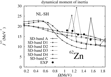
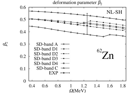
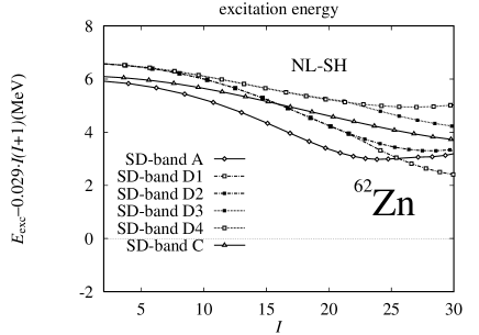
Figure 1:

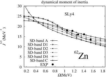
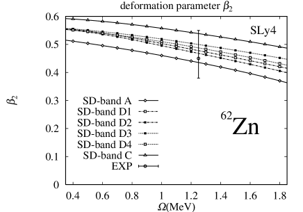
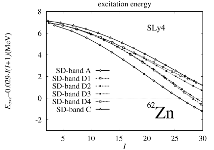
Figure 2:

Figure 3:

Figure 4:

References

- [1] P.J.Twin et al., Phys. Rev. Lett. 57 (1986) 811.
- [2] I.Ragnarsson, in: Proceedings of the Workshop on the Science of Intense Radioactive Ion Beams, Los Alamos, April 10-12 (1990) p.199.
- [3] C.E.Svensson et al., Phys. Rev. Lett. 79 (1997) 1233.
- [4] D.Rudolph et al., Phys. Rev. Lett. 80 (1998) 3018.
- [5] S.A.Chin and J.D.Walecka, Phys. Lett. B 52 (1974) 24.
- [6] J.D.Walecka, Ann. Phys. 83 (1974) 491.
- [7] S.A.Chin, Ann. Phys. 108 (1977) 301.
- [8] W.Koepf and P.Ring, Nucl. Phys. A 493 (1989) 61.
- [9] W.Koepf and P.Ring, Nucl. Phys. A 511 (1990) 279.
- [10] J.König and P.Ring, Phys. Rev. Lett. 71 (1993) 3079.
- [11] A.V.Afanasjev, J.König and P.Ring, Phys. Lett. B 367 (1996) 11.
- [12] A.V.Afanasjev, J.König and P.Ring, Nucl. Phys. A 608 (1996) 107.
- [13] J.König, Ph.D.thesis (1996) ,unpublished.
- [14] S.Weinberg, Gravitation and Cosmology: Principles and Applications of The General Theory of Relativity (John Willy and Sons, New York, 1972) p.365.
- [15] N.D.Birrell and P.C.W.Davies, Quantum Fields in Curved Space (Cambridge Univ. Press, London, 1982) p.81.
- [16] H.Madokoro and M.Matsuzaki, Phys. Rev. C 56 (1997) R2934.
- [17] J.König, private communication (1996).
- [18] Y.K.Gambhir, P.Ring and A.Thimet, Ann. Phys. 198 (1990) 132.
- [19] M.M.Sharma, M.A.Nagarajan and P.Ring, Phys. Lett. B 312 (1993) 377.
- [20] C.E.Svensson et al., Phys. Rev. Lett. 80 (1998) 2558.
- [21] J. Dobaczewski and J. Dudek, Comp. Phys. Commun. 102 (1997) 166.
- [22] J. Dobaczewski and J. Dudek, Comp. Phys. Commun. 102 (1997) 183.
- [23] J. Dobaczewski, e-print nucl-th/9801056 (1998).
- [24] E.Chabanat et al., Physica Scripta T 56 (1995) 231.
- [25] D.Rudolph et al., Nucl. Phys. A 630 (1998) 417c.
- [26] W.Nazarewicz et al., Nucl. Phys. A 435 (1985) 397.