Abstract

Starting from an unitary effective Lagrangian model for the meson-nucleon scattering developed in [1], we come to a unified description of both meson scattering and photon-induced reactions on the nucleon. To this end the photon is added perturbatively, yielding both Compton scattering and meson photoproduction amplitudes. In a simultaneous fit to all available data the parameters of the nucleon resonances are extracted. We find that a global fit to the data of the various channels involving the final states $\gamma N$, $\pi N$, $\pi\pi N$, $\eta N$ and $K\Lambda$ is possible. Especially in the eta photoproduction a readjustment of the masses and widths found in the fits to hadronic reactions alone [1] is necessary to describe the data. Only for the $D_{13}(1520)$ we find a possible disagreement for the helicity couplings extracted using the combined dataset and pion photoproduction multipoles alone. The model-dependence introduced by the restoration of gauge invariance is discussed and found to be significant mainly for resonances with small helicity couplings.

PACS: 14.20.Gk, 11.80Gw, 13.30.Eg, 13.75.Gx, 13.60.Le, 25.20.Lj
Keywords: baryon resonances; unitarity; partial wave analysis; meson photoproduction; Compton scattering; coupled channels

I Introduction

Photon- and meson-induced reactions on the nucleon are the main source of information about the nucleon resonance spectrum. From the knowledge of the possible excitations of the nucleon and their properties one hopes to extract information about the structure of the nucleon. To this end one needs models that allow to determine the masses and partial decay widths of the resonances. Because of the constraint of unitarity the different reaction channels can in principle not be treated separately, but have to be taken into account simultaneously.

For the purely hadronic reactions models based on unitarity and analyticity have been widely used [2, 3, 4, 5, 6, 7]. Using an ansatz developed by the Carnegie-Mellon Berkeley or CMB group, Dytman et al. for example have recently extracted resonance parameters from a fit to the $\pi N\to\pi N,\pi\pi N,\eta N$ data [8].

On the other hand, in calculations of meson photoproduction, effective Lagrangian models are the main tool for investigations [9, 10, 11, 12]. In these models the important constraint of gauge invariance can be easily implemented on the operator level. However, unitarity has only been fulfilled in a few calculations of pion photoproduction in the $\Delta$-region [9, 10, 13, 14] and eta photoproduction [12]. Lately, also a description of Compton scattering in this framework has been put forward [15].

With the availability of high-precision data from various accelerator facilities like MAMI, ELSA, GRAAL and TJNAF, there is also an urgent need to improve the models for meson photoproduction. The most important ingredient for these improved models is the dynamical treatment of the meson rescattering in the same framework as the initial photoproduction reaction. To this end a description of the purely hadronic reactions within the effective Lagrangian approach is necessary.

As a first step, we formulated a model for these hadronic reactions employing the $K$-matrix approximation [1]. The interaction potential is described solely in terms of $s$-, $u$- and $t$-channel Feynman diagrams. We have shown that a reliable extraction of the resonance parameters is possible in this model and that the effective Lagrangian approach reduces the number of free parameters considerably, since the non-resonant background is generated by a few couplings only.

Analyticity is not guaranteed in this approach, but there are estimates about the quality of the $K$-matrix calculation as compared to other approximations [4, 6]. These indicate that the final resonance parameters extracted in different approximations are very similar.

The aim of this paper is now, to extend this model to include also photon-induced reactions. This would allow to benefit from the very accurate data for such reactions that already are or will be available in the near future. To this end we will at first shortly discuss the model used and the results of the fits to hadronic data. The extension to photon-induced reactions and the database available for the various reactions will then be addressed. After that, the results of the fits to the combined data are presented and discussed.

An important new feature of this analysis is the extraction of electromagnetic coupling constants from a combined fit to meson photoproduction and Compton scattering data. Apart from the $t$-channel contributions, the latter is determined only by the electromagnetic couplings and not by a product of strong and electromagnetic couplings as in meson photoproduction. Compton scattering data should thus provide an important constraint on the extraction of electromagnetic coupling constants. We will also use a comparison with a dispersion theoretical analysis of these data to obtain information about the quality of the $K$-matrix approximation.

II Description of the model and its application to the purely hadronic reactions

For easier reference we review in this section briefly the treatment of the hadronic channels in [1]. This then forms the basis of our inclusion of photon-induced reaction channels.

A The $K$-matrix approximation

The Bethe-Salpeter equations encountered in meson-nucleon scattering

$$T=V+VG_{BS}T$$ (1)

can always be decomposed into two coupled equations [4, 16]:

$$K = V+V{\rm Re}(G_{BS})K$$ (2)

$$T = K-{\rm i}K{\rm Im}(G_{BS})T.$$ (3)

Here $G_{BS}$ is the Bethe-Salpeter propagator that describes the intermediate propagation of the meson and the nucleon.

In (3) the second equation can easily be solved, since the imaginary part of $G_{BS}$ is always proportional to $\delta$-functions that place the meson and nucleon on its mass-shell. The real part of $G_{BS}$ in the first equation in (3) amounts to a principle-value integral and is, therefore, much harder to treat.

The $K$-matrix approximation now consists of neglecting this principle-value integral in the first equation and thus using $K=V$ in the second one. This leads to

$$\left[T_{K}\right]=\left[V+{\rm i}VT_{K}\right]=\left[\frac{V}{1-{\rm i}V}\right],$$ (4)

where the brackets $[\cdots]$ indicate that $V$ and $T_{K}$ are $n\times n$-matrices ($n$ being the number of asymptotic channels taken into account) and that (4) is a matrix equation.

Obviously, $T_{K}$ as calculated from (4) does not necessarily fulfill a dispersion relation, as does the full $T$ from (3). Therefore, the $K$-matrix approximation does not guarantee analyticity by construction. However, Pearce and Jennings [4] have shown that in $\pi N$-scattering the contributions from ${\rm Re}(G_{BS})$ are of minor importance, since the corresponding principle-value integral is reduced by a very soft cutoff needed to regularize (3). Furthermore, Surya and Gross [6] estimated that in this process the error made by putting the pion onshell is of the order of $(E_{\pi}-m_{\pi})E_{\pi}^{3}/m_{N}^{4}$ and can therefore be neglected for small pion energies. Based on these studies, it seems that the main contributions in the Bethe-Salpeter equation (1) come from the rescattering with both intermediate particles onshell. This part is correctly taken into account in the $K$-matrix approximation.

B Contributions to the potential $V$

As asymptotic states $\pi N$, $\pi\pi N$, $\eta N$ and $K\Lambda$ have been taken into account. A detailed description of the database used in the fits is given in [1]. Neglected so far are final states such as $K\Sigma$ and $\omega N$. This has been done because either the coupling of resonances to this channel is known to be small ($K\Sigma$, [17]), or because only one resonance is known that might have a significant decay into this channel ($\omega N$, [5]).

Also the $\rho N$-channel is not contained in our analysis. To make at least partly up for this deficiency, we parameterize the $\pi\pi N$-decay by the coupling to a scalar, isovector $\zeta$-meson [1, 12, 13, 18] with mass $m_{\zeta}=2m_{\pi}$. This ensures that the important $\pi\pi N$-decay is taken into account, but at the same time the model is kept as simple as possible. A description of the $\pi\pi N$ final state in terms of two particle intermediate states like $\pi\Delta$, $\pi P_{11}(1440)$ and $\rho N$ is currently under way.

The potential $V$ is now calculated from the interaction Lagrangians collected in App. A. Taken into account are contributions from the nucleon Born terms, $t$-channel exchanges of $\rho$, $a_{0}$ and $K^{*}$ and resonance contributions in the $s$- and $u$-channels.

In this work we limit ourselves to partial waves with spin $\frac{1}{2}$ and $\frac{3}{2}$. This is because only for these the Lagrangians can be given in an unambiguous way [19, 20]. Furthermore, we restrict the energy range to $\sqrt{s}\leq$ 1.9 GeV because for higher energies additional decay channels might be important.

C Form factors

In order to investigate the dependence of the resonance parameters on the specific choice of the hadronic form factors, in [1] fits using combinations of the three basic forms

$$F_{p}(q^{2}) = \frac{\Lambda^{4}}{\Lambda^{4}+(q^{2}-m^{2})^{2}}$$ (5)

$$F_{e}(q^{2}) = \exp(-\frac{(q^{2}-m^{2})^{2}}{\Lambda^{4}})$$ (6)

$$F_{t}(q^{2}) = \frac{\Lambda^{4}+(q_{t}^{2}-m^{2}/2)^{2}}{\Lambda^{4}+(q^{2}-(q_{t}^{2}+m^{2}/2))^{2}}$$ (7)

have been carried out ($m$ denotes the mass of the propagating particle, $q$ its four-momentum and $q_{t}^{2}$ is the value of $q^{2}$ at the kinematical threshold in the $t$-channel). The following restrictions were imposed to limit the number of free cutoff parameters:

• the same functional form $F$ and cutoff $\Lambda_{N}$ is used in all vertices $\pi NN$, $\eta NN$ and $KN\Lambda$,

• for all resonances we take the same $F$ as for the nucleon, but different values $\Lambda_{1/2}$ and $\Lambda_{3/2}$ for the cutoffs for spin-$\frac{1}{2}$ and spin-$\frac{3}{2}$ resonances,

• in all $t$-channel diagrams the same $F$ and $\Lambda_{t}$ are used.

D Results for the hadronic reaction channels

In this section we briefly recapitulate the main results of the fits to the hadronic reactions $\pi N\to\pi N$, $\pi N\to\pi\pi N$, $\pi N\to\eta N$ and $\pi N\to K\Lambda$. The reader is referred to [1] for a more detailed discussion.

• A qualitative and quantitative description of all hadronic data is achieved.

• The resonance parameters we find are in good agreement with the values obtained by other groups [2, 3, 5, 7, 18] and with the PDG-values [17].

• The $\pi^{-}p\to\eta n$ data are not good enough to determine the $\eta N$-branching fractions of the nucleon resonances very accurately. Nevertheless, we find non-vanishing couplings for a few resonances ($S_{11}(1535)$, $P_{11}(1710)$, $P_{13}(1720)$ and $D_{13}(1520)$).

• Only two resonances ($S_{11}(1650)$ and $P_{11}(1710)$) exhibit sizeable couplings to the $K\Lambda$-channel. For higher energies the $\pi^{-}p\to K^{0}\Lambda$-reaction is dominated by the $t$-channel $K^{*}$-exchange.

• There are deviations from the $\pi N$ data for the $P_{I3}$- and $D_{I3}$-partial waves. Below the resonance positions we underestimate the amplitudes, whereas for energies above the resonance the fits give too large amplitudes. This indicates that a fit with form factors that are asymmetric around the resonance position $m_{R}$ (instead of our choices $F_{p,e}$) might lead to a better description of the data.

• Already for energies above 1.6 GeV we find that the $t$-channel contributions are not adequately described by the corresponding Feynman diagrams anymore. It seems that stronger modifications than those from any of the form factors $F_{p,e,t}$ are needed. A smooth transition to a Regge-like behavior in this energy range would probably improve the quality of the fits for the highest energies.

  Because of this, in the fits the $\pi NN$- and $\rho NN$-coupling constants are driven below their usual values. This in turn also leads to a smaller $P_{33}(1232)$ mass (1.229 GeV) and width (110 - 113 MeV).

A comparison with the resonance parameters obtained from other unitary and analytic analyses, as for example those listed in [17], shows that the hadronic reactions can be described rather well in this effective Lagrangian approach employing the $K$-matrix approximation.

III Extension to photon-induced reactions

With the inclusion of the $\gamma N$ final state a model can now be constructed that combines the advantages of describing the electromagnetic interactions using effective Lagrangians with a dynamical treatment of the rescattering. In principle this extension is straightforward, it mainly consists of enlarging the matrices $[V]$ and $[T]$ to take into account the new final state. Eq. (4) then gives the unitarized amplitudes for meson photoproduction and Compton scattering. However, there are four important points that make the combined treatment of all possible reaction channels technically more involved:

1. The photon can induce electric and magnetic transitions. Therefore, in the case of spin-$\frac{3}{2}$ resonances two amplitudes (called multipoles in photoproduction, instead of partial waves as in the hadronic reactions) have to be taken into account [16].

2. Furthermore, the interaction of the photon with the nucleon can be split up into an isoscalar and an isovector part. For e.g. pion photoproduction this leads to three different isospin amplitudes ($T^{0}$, $T^{1/2}$ and $T^{3/2}$), instead of two ($T^{1/2}$ and $T^{3/2}$) as in $\pi N$-scattering [16].

3. In the multipole-decompositions of photoproduction data any influence of Compton scattering is usually neglected [21].

4. The Compton amplitudes cannot be fully isospin-decomposed using experimental data alone. Since only two physical processes ($\gamma p$ and $\gamma n$) exist, only two of the four amplitudes can be extracted. Therefore, the rescattering contributions are normally calculated in a basis using physical states (e.g. $\pi^{-}p$, $\pi^{0}p$, $\pi^{+}n$, $\pi^{0}n$) and not pure isospin states [21].

The first point can easily be taken into account by introducing two new final states $(\gamma N)_{E}$ and $(\gamma N)_{M}$, where the index denotes the type of electromagnetic transition. The isoscalar/isovector nature of the photon can be treated in a similar way. The usual isospin decomposition of pion photoproduction, for example, is given by [12, 16]:

$$\langle\pi_{j}|T_{\pi\gamma}|\gamma\rangle=\tau_{j}T_{\pi\gamma}^{0}+\frac{1}{3}\tau_{j}\tau_{3}T_{\pi\gamma}^{1/2}+(\delta_{j3}-\frac{1}{3}\tau_{j}\tau_{3})T_{\pi\gamma}^{3/2}.$$ (8)

Here $T_{\pi\gamma}^{0}$ contains the amplitude for isoscalar photons, whereas $T_{\pi\gamma}^{1/2,3/2}$ are the amplitudes for total isospin $I\!=\!\frac{1}{2},\frac{3}{2}$ induced by isovector photons. The important point to note is, that rescattering of $T_{\pi\gamma}^{0}$ and $T_{\pi\gamma}^{1/2}$ takes place via the $I\!=\!\frac{1}{2}$ part of the hadronic reaction channels (e.g. $T_{\pi\pi}^{1/2}$), whereas for $T_{\pi\gamma}^{3/2}$ only $T_{\pi\pi}^{3/2}$ contributes. The $I\!=\!\frac{3}{2}$ amplitudes can, therefore, be treated in the usual way. For the $I\!=\!\frac{1}{2}$ sector a further splitting of the final states into $(\gamma N)_{E}^{0}$, $(\gamma N)_{E}^{1/2}$, $(\gamma N)_{M}^{0}$ and $(\gamma N)_{M}^{1/2}$ needs to be introduced.

The third and the fourth point amount to neglecting photon-rescattering contributions when extracting the photoproduction amplitudes from the data. Only a direct term $\sim V_{\gamma\gamma}$ is then present in Eq. (4). In our analysis of those amplitudes this can only be taken into account by using the form $T=V+{\rm i}TV$ and not $T=V/(1-{\rm i}V)$, since in the latter case direct and rescattering terms cannot be disentangled. For the photoproduction of a scalar meson $\varphi$ this schematically leads to

$$T_{\varphi\gamma}^{I_{\gamma}}=V_{\varphi\gamma}^{I_{\gamma}}+{\rm i}\sum\limits_{\varphi^{\prime}}T_{\varphi\varphi^{\prime}}^{I_{\varphi}}V_{\varphi^{\prime}\gamma}^{I_{\gamma}},\qquad I_{\gamma}=0,\frac{1}{2},\frac{3}{2},I_{\varphi}=\frac{1}{2},\frac{3}{2}.$$ (9)

For Compton scattering we end up with:

$$T_{\gamma\gamma}^{p,n}=V_{\gamma\gamma}^{p,n}+{\rm i}\sum\limits_{c}T_{\gamma c}V_{c\gamma}.$$ (10)

Here the sum runs over all physical intermediate states $c$ (e.g. $\pi^{0}p$, $\pi^{+}n$, … for $\gamma p\to\gamma p$). Neglected are in both cases contributions from the photon rescattering, since they are suppressed by an additional factor $e^{2}$. Because of the same suppression we also do not take electromagnetic corrections to the hadronic channel into account. We have checked this approximation by also calculating the photon-rescattering contributions in the $\Delta$-region and found them to be negligible.

A Background contributions and resonance couplings

The contributions to the potential $V$ in the case of photon-induced reactions come from Bremsstrahlung of asymptotic particles ($N$, $\pi$, $K$) and electromagnetic decays (e.g. nucleon resonances and vector mesons). The Bremsstrahlung leads to Born diagrams in the $s$-, $u$- and $t$-channels; decays of nucleon resonances give contributions in the $s$- and $u$-channels, whereas meson decays enter as $t$-channel diagrams.

To calculate the different contributions, we first of all need to specify the couplings to the photon. Since the Lagrangians have already been discussed many times [10, 9, 11, 12, 22], we limit ourselves to a short summary.

For the nucleon (N, $\Lambda$ and $\Sigma$) and the scalar mesons (denoted by $\varphi$) we have:

$${\cal L}_{\gamma NN} = -e\bar{N}\left[\frac{(1+\tau_{3})}{2}\gamma_{\mu}A^{\mu}-(\kappa^{s}+\kappa^{v}\tau_{3})\frac{\sigma_{\mu\nu}}{4m_{N}}F^{\mu\nu}\right]N$$ (11)

$${\cal L}_{\gamma N\Lambda,\Sigma} = e\bar{N}\kappa_{\Lambda,\Sigma}\frac{\sigma_{\mu\nu}}{4m_{N}}F^{\mu\nu}N$$ (12)

$${\cal L}_{\gamma\varphi\varphi} = -e\left[\mbox{\boldmath$\displaystyle\varphi$}\times(\partial_{\mu}\mbox{\boldmath$\displaystyle\varphi$})\right]_{3}A^{\mu}$$ (13)

$${\cal L}_{\gamma\varphi NN} = -e\frac{g_{\varphi NN}}{2m_{N}}\bar{N}\gamma_{5}\gamma_{\mu}\left[\mbox{\boldmath$\displaystyle\tau$}\times\mbox{\boldmath$\displaystyle\varphi$}\right]_{3}A^{\mu}.$$ (14)

The magnetic transitions moments are given by $\kappa_{\Lambda}=-0.613$ and $\kappa_{\Sigma}=1.610$ [17, 23]. In the case of pseudovector $\varphi NN$-coupling, ${\cal L}_{\gamma\varphi NN}$ gives rise to the so-called seagull- or 4-point-diagram.

For the decay of scalar ($\varphi$) and vector ($v$) mesons we use ($F^{\mu\nu}=\partial^{\nu}A^{\mu}-\partial^{\mu}A^{\nu}$, $v^{\lambda\sigma}=\partial^{\sigma}v^{\lambda}-\partial^{\lambda}v^{\sigma}$):

$${\cal L}_{\gamma\gamma\varphi} = e^{2}\frac{g_{\gamma\gamma\varphi}}{2m_{\varphi}}\varepsilon_{\mu\nu\lambda\sigma}F^{\mu\nu}(\partial^{\lambda}\varphi)A^{\sigma}$$ (15)

$${\cal L}_{\gamma\varphi v} = e\frac{g_{\gamma\varphi v}}{4m_{\varphi}}\varepsilon_{\mu\nu\lambda\sigma}F^{\mu\nu}v^{\lambda\sigma}\varphi,$$ (16)

with the couplings extracted from the corresponding decay widths [17]:

$$g_{\gamma\gamma\pi^{0}} = -0.044,\qquad g_{\gamma\gamma\eta}=0.167$$ (17)

$$g_{\gamma\pi^{0}\rho^{0}} = 0.131,\qquad g_{\gamma\pi^{\pm}\rho^{\pm}}=0.103,\qquad g_{\gamma\eta\rho^{0}}=1.020$$ (18)

$$g_{\gamma\pi^{0}\omega} = 0.313,\qquad g_{\gamma\eta\omega}=0.329$$ (19)

$$g_{\gamma\pi^{0}K^{*,0}} = 0.631,\qquad g_{\gamma\pi^{\pm}K^{*,\pm}}=0.415.$$ (20)

For the spin-$\frac{1}{2}$ resonances only a magnetic transition is possible:

$${\cal L}_{\gamma NR_{1/2}}=e\bar{R}g_{1}\frac{\Gamma_{\mu\nu}}{4m_{N}}NF^{\mu\nu}+h.c.,$$ (21)

where $R$ is the resonance spinor. The operator $\Gamma_{\mu\nu}$ is given by $\gamma_{5}\sigma_{\mu\nu}$ for odd-parity resonances and by $\sigma_{\mu\nu}$ otherwise. In the spin-$\frac{3}{2}$ case two couplings can contribute:

$${\cal L}_{\gamma NR_{3/2}} = -\frac{{\rm i}eg_{1}}{2m_{N}}\bar{R}^{\alpha}\Theta_{\alpha\mu}(z_{1})\gamma_{\nu}\Gamma NF^{\nu\mu}+$$ (23)

$$-\frac{eg_{2}}{4m_{N}^{2}}\bar{R}^{\alpha}\Theta_{\alpha\mu}(z_{2})\Gamma(\partial_{\nu}N)F^{\nu\mu}+h.c.,$$

$$\Theta_{\alpha\mu}(z) = g_{\alpha\mu}-\frac{1}{2}(1+2z)\gamma_{\alpha}\gamma_{\mu}.$$ (24)

Here, the operator $\Gamma$ is either $1$ or $\gamma_{5}$ for odd and even parity resonances, respectively.

The initial values for the electromagnetic couplings of the resonances are calculated from the helicity couplings given by the Particle-Data-Group [17]. The connections between the $g_{1,2}$ used here and the $A_{1/2,3/2}$ are as follows [24, 25]:

Spin-$$\frac{1}{2} A_{1/2}=\mp\frac{e\xi_{R}}{2m_{N}}\sqrt{\frac{m_{R}^{2}-m_{N}^{2}}{2m_{N}}}g_{1}$$ : (25)

Spin-$$\frac{3}{2} A_{1/2}=-\frac{e\xi_{R}}{4m_{R}}\sqrt{\frac{m_{R}^{2}-m_{N}^{2}}{3m_{N}}}(\pm g_{1}+\frac{m_{R}}{4m_{N}^{2}}(m_{R}\mp m_{N})g_{2})$$ : (27)

$$A_{3/2}=\mp\frac{e\xi_{R}}{4m_{N}}\sqrt{\frac{m_{R}^{2}-m_{N}^{2}}{m_{N}}}(g_{1}-\frac{1}{4m_{N}}(m_{R}\mp m_{N})g_{2}).$$

Here $\xi_{R}$ denotes the phase at the $\pi NR$-vertex. These relations can easily be inverted to extract the $g_{1,2}$.

In all these couplings we have to account for the isoscalar/isovector nature of the photon. This is done in the case of $I\!=\!\frac{1}{2}$ resonances by using $g_{1,2}=g^{s}_{1,2}+\tau_{3}g^{v}_{1,2}$ in (21) and (23). Note that $I\!=\!\frac{3}{2}$ resonances only couple to isovector photons and therefore have the same coupling $g_{1,2}T_{3}$ to $\gamma p$ and $\gamma n$.

The formulae needed for the multipole decomposition of photoproduction and Compton scattering are somewhat lengthy and have been collected in App. B. There we also list the connections of the amplitudes to the various observables.

B Form factors and gauge invariance

As we have already stated in the introduction, an effective Lagrangian model allows to address the question of gauge invariance on a fundamental level. Unfortunately, there is no unique way to restore gauge invariance once hadronic form factors have been introduced. This ambiguity affects only the Born terms, since all transition vertices fulfill gauge invariance by construction [9]. That is, having a vertex function $\Gamma^{\mu}_{RN\gamma}$ constructed from the corresponding Lagrangian, we always have

$$\Gamma^{\mu}_{RN\gamma}k_{\mu}=0,$$ (28)

where $k_{\mu}$ is the photon-momentum. The main reason for this is that a $R\to N\gamma$ transition cannot be derived from the hadronic Lagrangians by minimal substitution, but has to be constructed by hand. Therefore, all corresponding vertex functions have to fulfill (28) separately, in order to preserve gauge invariance. Because of this, we have also introduced independent form factors at the electromagnetic vertices of the nucleon resonances. These form factors are taken to have the same analytic form as the hadronic ones (cf. Eq. (7)), only the cutoffs $\Lambda$ are chosen independently.

For vertices derived through minimal substitution, only the sum of all contributing ($s$-, $u$- and $t$-channel and 4-point) diagrams needs to fulfill a constraint similar to (28):

$$\sum\limits_{i=s,u,t,4}{\cal M}_{\gamma\varphi,i}^{\mu}k_{\mu}=0.$$ (29)

Here ${\cal M}_{\gamma\varphi,i}^{\mu}$ denotes the contribution of the $i$’th Born diagram to the photoproduction amplitude.

In the case of pion photoproduction the vertex functions are $\Gamma^{\mu}_{\gamma NN}$, $\Gamma^{\mu}_{\gamma\pi\pi}$ and $\Gamma^{\mu}_{\gamma\pi NN}$ and lead to four possible diagrams: $s$-, $u$- and $t$-channel and 4-point. Now the momenta at the hadronic vertices are different in all diagrams. Since, correspondingly, the form factors have different values for each diagram, all terms in (29) are weighted differently once hadronic form factors are introduced. Hence, the inclusion of any of the factors $F_{p,e,t}$ will results in a violation of gauge invariance.

The first model that tries to solve this problem was proposed by Ohta [26]. In his ansatz it is assumed that the form factor $F$ can be separately Taylor-expanded with respect to the momenta $p$ $p^{\prime}$ and $q$. After minimal substitution in all three momenta, the resulting expressions can then be resummed in closed form.

To illustrate this in some detail, we focus on the $s$-channel Born diagram. For our choice of hadronic form factors the amplitude ${\cal M}_{\gamma\pi,s}^{\mu}$ is given by (suppressing factors of ${\rm i}$):

$${\cal M}_{\gamma\pi,s}^{\mu}={\bar{u}}(p^{\prime})g_{\pi NN}F(s)\gamma_{5}q\!\!\!/\frac{(p\!\!\!/+k\!\!\!/)+m_{N}}{(p+k)^{2}-m_{N}^{2}}e\left[\gamma^{\mu}+\frac{{\rm i}\sigma^{\mu\nu}}{2m_{N}}\kappa_{N}k_{\nu}\right]u(p).$$ (30)

Using now Ohta’s prescription we obtain an additional counter term $\left.{\widetilde{\cal M}}_{\gamma\pi,s}^{\mu}\right|_{Ohta}$. After some rearrangements the sum of both can be expressed as:

$$\left.{\cal M}_{\gamma\pi,s}^{\mu}\right|_{Ohta} = {\cal M}_{\gamma\pi,s}^{\mu}+\left.{\widetilde{\cal M}}_{\gamma\pi,s}^{\mu}\right|_{Ohta}=$$ (32)

$${\bar{u}}(p^{\prime})g_{\pi NN}\gamma_{5}q\!\!\!/\frac{(p\!\!\!/+k\!\!\!/)+m_{N}}{(p+k)^{2}-m_{N}^{2}}e\gamma^{\mu}u(p)+\mbox{Terms }\sim\sigma^{\mu\nu}k_{\nu}.$$

From this it is clear that the influence of the form factor $F$ on the coupling to the charge of the nucleon has been fully removed by the Ohta-prescription. Only the coupling to the magnetic moment (which is gauge invariant by itself) is affected by the introduction of $F$ at the hadronic vertex. The same also holds for the $u$- and $t$-channel diagrams.

Haberzettl [27] has argued against this procedure because four-momentum conservation connects $p$, $p^{\prime}$ and $q$ and the form factor $F$ is needed at an unphysical point $F(m_{N}^{2},m_{N}^{2},m_{\varphi}^{2})$. To incorporate both points, he has developed an alternative method that leads to different expressions for the final amplitude.

If we choose, for example, $p$ and $p^{\prime}$ as the independent variables, we can remove the $q$-dependence by using $q=p^{\prime}-p$. After this, we get one counter-term less than in Ohta’s method. The net result for the electric $s$-channel contribution is in this case given by:

$$\left.{\cal M}_{\gamma\pi,s}^{\mu}\right|_{Haberzettl}=\left.{\cal M}_{\gamma\pi,s}^{\mu}\right|_{Ohta}\cdot F(t).$$ (33)

Instead of removing the influence of $F$ altogether, we now have replaced the form factor used in the bare Born diagram with the one from the $t$-channel exchange. Since the same happens for the other diagrams as well, we have an overall factor $F(t)$ multiplying the charge contributions from all four Born diagrams. Of course, the choice of independent variables is arbitrary, so that in its most general form the amplitude (33) contains, instead of $F(t)$, a common form factor ${\widetilde{F}}={\widetilde{F}}(s,u,t)$. This degree of freedom has for example been used in the calculation of Nozawa et al. [9], where a form factor ${\widetilde{F}}=F(s)$ was taken into account. Following Haberzettl [27], we use here an ansatz of the form

$${\widetilde{F}}(s,u,t)=a_{1}F(s)+a_{2}F(u)+a_{3}F(t),$$ (34)

with the additonal constraint $a_{1}+a_{2}+a_{3}=1$; in [27] the coefficients $a_{i}$ were fitted in kaon photoproduction.

To investigate the dependence of the electromagnetic couplings of the resonances on the gauge procedure, we have performed fits using both Ohta’s method and the prescription of Haberzettl. Since this is mainly an exploratory study we have in the latter case adopted the ‘democratic’ choice and taken the $a_{i}$’s to be equal. For pion photoproduction this leads to the ansatz ${\widetilde{F}}(s,u,t)=1/3(F(s)+F(u)+F(t))$ (34). In the case of eta and kaon photoproduction, however, we use a slightly different form factor ${\widetilde{F}}$ because in both cases the Born terms consist of a smaller number of diagrams. For the eta case we don’t have a $t$-channel contribution, whereas for the kaon photoproduction there is no $u$-channel diagram involving a coupling to the charge of the particles. Therefore, in our calculation the ansatz

$$\begin{array}[]{lclclcl}{\widetilde{F}}_{\pi}(s,u,t)&=&\frac{1}{3}F(s)&+&\frac{1}{3}F(u)&+&\frac{1}{3}F(t)\\ {\widetilde{F}}_{\eta}(s,u)&=&\frac{1}{2}F(s)&+&\frac{1}{2}F(u)\\ {\widetilde{F}}_{K}(s,t)&=&\frac{1}{2}F(s)&+&&&\frac{1}{2}F(t),\end{array}$$ (35)

was used for the different form factors. This prescription has been chosen to avoid additional free parameters. But we want to stress again that (34) and (35) can only be motivated by the structure of the hadronic vertices present in the photoproduction diagrams. Only in a microscopic model for the electromagnetic vertex the form factor could be determined unambiguously.

Finally, one could think about introducing form factors at the electromagnetic vertices of the nucleon and the pion and kaon as well. For the $\gamma NN$ case this would lead to the following vertex:

$$\Gamma_{\gamma NN}^{\mu}={\bar{u}}(p^{\prime})e\left[F_{1}(p^{2},p^{\prime\,2},k^{2})\gamma^{\mu}+F_{2}(p^{2},p^{\prime\,2},k^{2})\frac{{\rm i}\sigma^{\mu\nu}}{2m_{N}}k_{\nu}\right]u(p)$$ (36)

For real photons gauge invariance demands $F_{1}(p^{2},p^{\prime\,2},0)=1$. In addition, for $F_{2}$ we have $F_{2}(m_{N}^{2},m_{N}^{2},0)=\kappa_{N}$. Besides this, we have no further constraint on $F_{2}$ for the case of meson photoproduction. In the case of Compton scattering it can be shown [28], however, that additional contributions are needed to restore gauge invariance, once a form factor $F_{2}$ has been introduced. Unfortunately, also these contributions cannot be determined in an unambiguous way. To avoid this additional uncertainty, we have chosen not to include electromagnetic form factors for the nucleon and scalar mesons in our calculation.

C Calculation of photon-induced reactions

The calculation of photon-induced reactions is now carried out as follows: i) calculate the potential $[V]$ from all contributing Feynman diagrams; ii) invert the hadronic submatrix to give the $T$-matrix $[T_{hadr}]=[V_{hadr}/(1-{\rm i}V_{hadr})]$; iii) unitarize the meson photoproduction with the help of (9); iv) finally, calculate the $T$-matrix for Compton scattering using (10).

The potential $[V_{hadr}]$ is calculated using the results of [1], with only one exception: at the $\eta NN$-vertex we now use pseudoscalar (PS) instead of pseudovector (PV) coupling. From eta photoproduction [29] it is known that PS coupling leads to a much better description of the data. In purely hadronic reactions this PS $\leftrightarrow$ PV difference is hardly visible because of the suppresion of the Born terms due to the hadronic form factor. But since, at least for the Ohta-prescription, the influence of the form factor is removed by restoring gauge invariance, in photoproduction the contribution of the Born terms is enhanced as compared to others. For kaon photoproduction the situation is not so clear [30], so we will use both PS and PV coupling at the $KN\Lambda,\Sigma$-vertices in the fits.

D Summary of the model

Our model thus consists of a $K$-matrix treatment of the following asymptotic channels: $\pi N$, $\pi\pi N$, $\eta N$, $K\Lambda$, and $\gamma N$. The $K$-matrix elements are calculated from a Lagrangian given in [1] for the hadronic couplings and in the present paper for the electromagnetic couplings. Possible intermediate states are the nucleon and all three-star nucleon resonances with spins 1/2 and 3/2 up to an invariant mass of $\sqrt{1.9}$ GeV; thus no nucleon resonances appear in the final states of a Feynman diagram. As a consequence of the $K$-matrix approximation all intermediate particles propagate only on-shell.

With these ingredients all Feynman-amplitudes are calculated taking into account the $s$-, $u$- and $t$-channel diagrams. The latter are used to consistently generate the background amplitudes thus eliminating the need to introduce separate ad-hoc background parametrizations. The iteration of the amplitude $V$ contained in Eq. (4) then leads to a consistent description both of resonance decay widths and rescattering in a hadronic reaction. For example, in a reaction with asymptotic channels $\gamma N\rightarrow\eta N$ a whole chain of rescatterings, like e.g., $\gamma N\rightarrow N^{*}\rightarrow\pi N\rightarrow N^{**}\rightarrow\eta N$, where $N^{*}$ and $N^{*}*$ are different nucleon resonances, is automatically generated. While the resonances in this way all acquire width, and are thus ‘dressed’, higher order contributions to the vertices are not taken into account and the extracted couplings therefore are ‘bare’ ones.

IV Results of the fits

The parameters of the model can be grouped into resonant and non-resonant ones. The first group is given by the masses and the hadronic and electromagnetic couplings of the resonances. Furthermore, it also contains the $z$-parameters of the spin-$\frac{3}{2}$ resonances and the cutoffs $\Lambda$ of the form factors at all vertices. In the case of the non-resonant background we have the couplings of the scalar and vector mesons to the nucleon and the cutoffs at those vertices. The vector meson decays are calculated with the couplings fixed to (20). Only $g_{\gamma\eta\rho^{0}}$ and $g_{\gamma\eta\omega}$ have been allowed to vary in the fits because the corresponding decay widths are only known to about 25%.

As has been explained in Sec. II B, only resonances with spin $\frac{1}{2}$ and $\frac{3}{2}$ have been taken into account. These are: $S_{11}(1535)$, $S_{11}(1650)$, $P_{11}(1440)$, $P_{11}(1710)$, $D_{13}(1520)$, $D_{13}(1700)$, $S_{31}(1620)$, $P_{33}(1232)$, $P_{33}(1600)$ and $D_{33}(1700)$. Furthermore, the potential contains $t$-channel contributions from the hadronic and electromagnetic decays of the vector mesons $\rho$, $\omega$, $a_{0}$ and $K^{*}$. For the coupling of the $\omega$ to the nucleon, the values

$$g_{\omega NN}=7.98,\qquad\kappa_{\omega NN}=-0.12$$ (37)

have been used [9, 22]. The dependence of the electromagnetic couplings of the $P_{33}(1232)$ on the $\omega NN$-couplings have been investigated in [10, 13, 14]. Mainly due to the $\omega$-exchange contributions to the $M_{1+}^{3/2}$-multipole both couplings $g_{1}$ and $g_{2}$ of the $P_{33}(1232)$ are influenced by variations in $g_{\omega NN}$ and $\kappa_{\omega NN}$. Therefore, also the extracted $E/M$-ratio is somewhat sensitive to the values of those couplings. In principle one could go ahead and also determine $g_{\omega NN}$ and $\kappa_{\omega NN}$ through fits to the data. However, we have not chosen to do so, because we feel that the pion photoproduction data alone do not offer enough sensitivity to reliably determine the $\omega NN$-couplings. In view of the aim of this study to find a simultaneous description of all included channels the so induced error in the $P_{33}(1232)$-couplings is acceptable.

A Reaction channels and database

The hadronic database has been described in [1] and consists of PWA results for both $\pi N\to\pi N,\pi\pi N$ [3, 5, 7] and cross section and polarization data for $\pi^{-}p\to\eta n,K^{0}\Lambda$. Because of the much larger database used in the SM95-PWA as compared to the KA84-solution, we only use the SM95 data and the corresponding parameter set of [1] in this calculation.

• $\displaystyle\gamma p\to\gamma p$: Differential cross section data from various measurements [31] have been used in the fits. Furthermore, we include the LEGS data on photon polarizations [32], the old data on the recoil polarization from Wada et al. [31] have not been used here. Since, from the helicity couplings given in [17], we expect sizable contributions from spin-$\frac{5}{2}$ resonances ($D_{15}(1675)$ and $F_{15}(1680)$) not taken into account here, we fit the Compton data only for energies $<$ 1.6 GeV. Only in this energy range we can be sure that all resonance contributions are taken into account.

• $\displaystyle\gamma N\to\pi N$: In this channel we use the single-energy data of the multipole analysis SP97 [7]. In principle, also another analysis (MA97 [33]) is available, based mainly on the latest MAMI and ELSA data. This analysis, however, only covers the energy region $<$ 1.35 GeV. Because of this restriction, we do not use it in our fits. Nevertheless, differences between the two solutions SP97 and MA97 and our fits are shown in some of the plots. In a later stage of the investigation it would be very interesting to perform restricted fits using the MA97 data. This could allow to investigate the dependence of the $P_{33}(1232)$ couplings on the multipole analysis used.

  Unfortunately, the spreading of the single-energy data SP97 is much larger than for the $\pi N$-analysis SM95. In order to further restrict the parameters, we also use the speeds calculated from the energy-dependent solution SP97 in our fits. However, some precautions are necessary when incorporating these data, in particular near the resonance positions of the $P_{11}(1710)$ and the $D_{13}(1700)$. Even though a resonant structure cannot be ruled out from the SP97 single-energy solution, the SP97 speed data are smooth in the vicinity of both resonances. In our calculation, however, we always find resonant structures, even for resonances coupling only weakly to $\gamma N$. For energies near these resonances, therefore, no fit to the SP97 speeds is possible. For this reason the speed data for the resonant multipoles were not used near the $P_{11}(1710)$ and the $D_{13}(1700)$ in our fit.

• $\displaystyle\gamma N\to\eta N$: In the energy range below 1.54 GeV we only use the very precise data of Krusche et al. [34] for the differential and total cross section. For energies above that only sparse data from different groups are available [35]. For the total cross section there are also data from ELSA [36] for eta electroproduction at very small $k^{2}$ (= $-$0.056 GeV²), but no differential cross sections. From measurements on deuterium targets also neutron to proton ratios have been extracted [37]. Furthermore, a few target asymmetry data are available [38]. The latest measurements at GRAAL on photon asymmetries, however, are not yet published.

• $\displaystyle\gamma p\to K^{+}\Lambda$: Here, the best data come from the SAPHIR experiment [39]. The older measurements of differential cross sections and $\Lambda$-polarizations [40] have been carefully investigated by Adelseck and Saghai [23]. Because of systematic deviations of certain datasets, the errorbars of these data have been enlarged. In our fits we also use these newly assigned errors.

The fits are labeled (as in [1]) by the $\pi N$-PWA used to determine the hadronic parameters and the type of form factors for the $s$- and $t$-channel resonances. An additional number indicates the method used to gauge the Born contributions: 1 - Ohta’s method [26] with fixed hadronic parameters, 2 - Ohta’s method with all parameters fitted and 3 - Haberzettl’s method [27] with fixed $a_{i}$’s (cf. Eq. (35)). Furthermore, from the fits performed for the hadronic channels, it is obvious that the exponential form $F_{e}$ leads to larger values of $\chi^{2}$ as compared to the other form factors $F_{p}$ and $F_{t}$. Therefore, we do not use the parameterization $F_{e}$ for the case of photon-induced reactions. Finally, since the fits performed in [1] using $F_{p}$ and $F_{t}$ lead to very similar descriptions of the data, we limit ourselves to fits starting from the parameter set SM95-pt (given in [1] and also in the Tables III - V). Here one must keep in mind that the use of different parameterizations for the form factors introduces a source of systematic error that can be of comparable size to the statistical uncertainty induced by the error of the data.

In summary, the fit results are then labeled by SM95-pt-1, SM95-pt-2 and SM95-pt-3, standing for the SM95 partial wave analysis of $\pi N$ scattering of the Virginia group [7], all using the form factor $F_{p}$ from Eq. (7) for all vertices with propagating hadrons and $F_{t}$ from the same equation for the $t$-channel diagrams. They employ Ohta’s gauge fixing method with hadronic parameters determined from a fit to hadronic channels alone, Ohta’s gauge fixing method with all parameters refitted to all channels, including the photonuclear ones, and Haberzettl’s gauge fixing method, respectively.

B Fit with fixed hadronic parameters

In a first fit, we allowed only the electromagnetic couplings to vary. All other values of masses and decay widths were taken from the parameter set SM95-pt of [1]. Using the procedure of Ohta to restore gauge invariance, the parameters have been determined by a simultaneous fit to the full database as described above.

In Figs. 1 - 9 we show the results of this fit as dotted lines, together with the other fits described below. From the plots it is clear that the experimental data in all channels can be reproduced rather well. The improvement over our old non-unitary calculation [22] using the $T$-matrix approximation (also shown in Figs. 1 - 3) is obvious.

a Comparison to a $T$-matrix calculation

One of the most noticeable differences between the calculations performed here and those in Ref. [22] is the improvement in the description of the $E_{1+}^{3/2}$- and $M_{2-}^{n}$-multipoles. In the case of $E_{1+}^{3/2}$, it is well known that only a correct treatment of the rescattering allows a quantitative description of this channel. The reason for this can best be seen in Fig. 10, where a calculation with both $P_{33}(1232)N\gamma$-couplings set to zero is shown. Even with no direct coupling to the resonance, the structure of the data in the $E_{1+}^{3/2}$-multipole can already be reproduced quite well. This shows that the rescattering is responsible for the shape of this multipole and not the direct excitation of the $\Delta$. From this it is obvious, why our old model [22] failed in describing this multipole.

In [22] we have speculated that the same might be true for the $M_{2-}^{n}$-multipole, but Fig. 10 shows that this is not the case. The direct coupling of the resonance is essential to describe the data for both $E_{2-}^{n}$- and $M_{2-}^{n}$-multipoles. Therefore, the poor fit in the old calculation was obviously driven by the contributions of the $D_{13}(1520)$ to some other multipole. These were most likely the offshell contributions that are not treated correctly in the $T$-matrix approximation. One important deficiency in this approximation is the appearance of spurious resonance-like structures (e.g. $E_{1+}^{p,n}$, $M_{1+}^{p,n}$, $E_{0+}^{3/2}$ and $M_{1-}^{3/2}$). These are induced by the offshell contributions of the spin-$\frac{3}{2}$ resonances. As has been demonstrated in [1], these structures are an artifact of the $T$-matrix approximation and do not appear in a unitary calculation. Therefore, the investigation of offshell contributions of spin-$\frac{3}{2}$ resonances and the corresponding $z$-parameters, as has been done recently by Mizutani et al. [41], is not very meaningful in a $T$-matrix calculation. Without dynamical rescattering, the $z$-parameters are mainly adjusted to minimize the induced offshell-structures and reveal only little about the nature of the spin-$\frac{3}{2}$ resonances. From what we have said about the $M_{2-}^{n}$-multipole, it furthermore seems that also some resonance couplings are influenced by this effect.

Also, the dynamical generation of the imaginary parts of the amplitudes leads to an improved fit. Especially in cases where the Born terms dominate the amplitude, the old calculation did not generate the correct imaginary part ($E_{0+}$, $E_{1+}^{p,n}$ and $M_{1+}^{p,n}$). This is also easily understood, since in the $T$-matrix approach the Born terms are purely real.

b Compton scattering

This is the one of the first attempts to calculate Compton scattering in a dynamical model beyond the $\Delta$ resonance. Therefore, we are for the first time able to check if the data on Compton scattering and meson photoproduction can be described using the same helicity couplings for the various resonances. As can be seen from Fig. 9, we are able to fit the available data on Compton scattering very well. Both the differential cross section and the photon asymmetry $\Sigma$ are reproduced over the whole energy range. From this we conclude that the Compton data are indeed compatible to the experimental results for the photoproduction channels.

The main contributions to the cross section come from the Born $s$- and $u$-channel diagrams and the resonances $P_{33}(1232)$ and $D_{13}(1520)$. This can be seen from Fig. 11, where a decomposition of the differential cross section into the individual contributions is shown. It is also obvious that the $\pi^{0}$ and $\eta$ $t$-channel diagrams have a small influence under backward angles only. For energies below 1.6 GeV all other resonance contributions could be safely neglected, none of them exceeds 5 nb/sr.

Furthermore, in our calculation there is no need for an additional attenuation factor for the Born terms, as introduced by Ishii et al. [31] ($x=\cos\theta$):

$${\widetilde{A}}_{Born}=A_{Born}{\rm e}^{-C(1-x)},$$ (38)

with a free parameter C fitted to the Compton data. The strong backward peaking of the Born contributions is an artifact of the $T$-matrix approximation employed by Ishii et al. and does not persist once the amplitudes are properly unitarized. To illustrate the difference between the $K$- and $T$-matrix calculation, we show in Fig. 12 the Born $s$- and $u$-channel contribution to the differential cross section employing both $K$- and $T$-matrix approximation. The inclusion of mainly $\pi N$ rescattering leads to an enhancement of the cross section under forward angles and to the abovementioned reduction under backward angles. Therefore, we are able to fit the Compton data without an additional factor ${\rm e}^{-C(1-x)}$.

For the photon asymmetry $\Sigma$ we also show the results of the isobar model of Wada et al. [31] in the lower part of Fig. 9. Obviously, this ansatz is not able to describe the data. Both magnitude and shape are in disagreement with the experimental results. The dispersion relation calculations of L’vov [42], on the other hand, can reproduce the polarization data very well. In this region they practically coincide with our results, whereas for energies $\sqrt{s}\approx$ 1.08 GeV both approaches differ by a factor of two.

This observation allows us to investigate the validity of the $K$-matrix approximation in some detail. The main difference to the dispersion relation calculation performed in [42] is the onshell-approximation for $G_{BS}$ in Eq. (3). Therefore, in our calculation the $\pi N$ intermediate state does not contribute below $m_{N}+m_{\pi}\approx$ 1.08 GeV. Taking also the offshell-propagation into account (as the dispersion relation implicitly does), the Compton scattering ‘sees’ the $\pi N$-channel already for lower energies. This is the main reason for the different results in $\Sigma$ within about 50 MeV around the $\pi N$-threshold. We thus conclude that the offshell ‘tails’ of the propagator $G_{BS}$ do not extend much further than $\approx$ 50 MeV. This observation is in agreement with the results of Pearce and Jennings [4], who found that a rather soft offshell-cutoff in $G_{BS}$ is needed ($\Lambda\approx$ 300 MeV) to describe the $\pi N$-phasehifts. Thus, it seems that the $K$-matrix approximation yields reliable results for energies not too close to a meson-production threshold.

c Eta photoproduction

Looking at the overall result from our fit, we find that all major structures of the data are also visible in the calculation. Only for a few channels significant deviations from the data can be seen. The most prominent of these can be found in eta photoproduction below 1.6 GeV (cf. Figs. 4 and 5). As we have pointed out earlier, especially in this region high precision measurements are already available [34]. Since the forthcoming experiments should yield data with comparable quality, the eta photoproduction can be seen as a ‘testing ground’ for all models that try to describe photon-induced reactions. Only the full description of this data in all details might allow the unambiguous extraction of the $S_{11}(1535)$ resonance parameters.

From the differential cross section it is clear that mainly the absolute magnitude is too small for energies below 1.5 GeV, whereas the isotropy is well reproduced. Therefore, an increase of the $S_{11}(1535)p\gamma$-coupling alone would not improve the overall fit, since it would lead to a drastic over-prediction of the data for energies above 1.5 GeV. From this we conclude that a change in the energy dependence of the resonance contribution is needed for a better fit in this channel. Such a change can only result from a variation of the hadronic masses and couplings; the coupling to the photon mainly influence the magnitude and not the shape of the $S_{11}(1535)$ contribution.

This observation coincides with the fact that the poor $\pi^{-}p\to\eta n$ data were responsible for the spread of the $S_{11}(1535)$ parameters between the different fits carried out in [1]. Also the smaller $\eta N$-couplings of the other resonances could not be extracted reliably. In the moment, it seems that the eta photoproduction imposes much stricter constraints on the resonance parameters, as the purely hadronic data does. This clearly shows that new precise photoproduction measurements need to be accompanied by improved hadronic data as well. Otherwise, extractions of resonance parameters will always be handicapped by the quality of the hadronic database.

d Kaon photoproduction

In the other reaction channels this problem does not show up, mainly because of the lack of high precision data. Only in the case of kaon photoproduction for energies around 1.75 GeV we have indications of systematic deviations in backward directions. Here the cross section is dominated by the Born contributions, since $g_{K\Lambda N}$ is rather large ($\approx$ $-$6, e.g. compared to $g_{\eta NN}\approx$ 1-2). In the hadronic channels only the product of coupling constant and hadronic form factor enters, which is much smaller ($\approx$ $-$2.5 in the case of $g_{K\Lambda N}$). Additionally, $\pi^{-}p\to K^{0}\Lambda$ is for higher energies dominated by the $K^{*}$-exchange in the $t$-channel. So the Born contribution, and thus $g_{K\Lambda N}$, is not well determined by the hadronic data.

In the kaon photoproduction, however, $g_{K\Lambda N}$ plays a dominant role, since in the Ohta prescription the influence of the hadronic form factor is completely removed. Furthermore, the contribution from the charge of the proton is not cancelled by a similar $u$-channel contribution, as it is the case in $\pi^{0}$ production. Because of the hidden strangeness in the $K\Lambda$ final state, we have a $\Lambda$ (or $\Sigma$) propagating in the crossed diagram that only exhibits magnetic coupling (as in $\pi^{+}$ production). Since all major contributions are therefore fixed from the outset, the fit could only be improved by reducing the photon coupling of the $S_{11}(1650)$. The resulting value ($A_{1/2}^{p}=31\!\times\!10^{-3}$ GeV^-1/2) is significantly smaller than the number deduced from pion photoproduction ($A_{1/2}^{p}=69\!\times\!10^{-3}$ GeV^-1/2, [7]). In our fit to the combined data of both channels the $E_{0+}^{p}$ data on pion photoproduction obviously do not play such an important role as the kaon photoproduction data because of the large uncertainty of the former in the region of the $S_{11}(1650)$.

Already with fixed hadronic parameters we obtain a good overall fit. From the observed deviations it is clear that a further improvement can only be achieved by simultaneously varying some of the hadronic parameters as well. Before we show the results for such combined fits, we want to stress again that already with fixed hadronic parameters a reasonable description of all data is possible. Especially due to the dynamical rescattering, the main shortcomings of a $T$-matrix calculation have been resolved.

C Global fit using Ohta’s prescription

In this section we now discuss the results of a global fit to all hadronic and photon-induced channels in which also the hadronic parameters are allowed to vary. Ohta’s prescription was used to gauge the hadronic form factors. The results are also shown in Figs. 1 - 9.

a Compton scattering

Looking at the plots for the different reaction channels, we in general find only a slight improvement using SM95-pt-2. In the case of Compton scattering, the fit with fixed hadronic parameters already describes the data rather well, so that the new fit leads only to a relatively small decrease in $\chi^{2}_{\gamma\gamma}$ (7.15 $\to$ 5.20). Since the main contributions here come from the Born terms and the $P_{33}(1232)$ and $D_{13}(1520)$ resonance, the changes in the differential cross sections can easily be explained by the slightly different helicity couplings found in both fits. For the $P_{33}(1232)$ both $A_{1/2}$ and $A_{3/2}$ are reduced and lead to the observed reduction for energies up to 1.3 GeV. In contrast to this, the increase in the $D_{13}(1520)$ helicities increases the interference with the other contributions to Compton scattering. Therefore, the cross section is reduced slightly in this case as well.

b Pion photoproduction

For the pion photoproduction the reduction of $\chi^{2}_{\gamma\pi}/DF$ is due to a the better fit of the $M_{1+}^{3/2}$-multipole. The increase in $\chi^{2}_{\pi\pi}/DF$ comes mainly from the $S_{11}$-channel, since the $S_{11}(1535)$-parameters exhibit the largest changes as compared to the SM95-pt-1 values. Except from this we note only minor changes, mainly for channels where the background is dominated by the Born contribution (e.g. $M_{1-}$, and $E_{1+}^{p,n}$). Accordingly, the values for the helicity couplings we extract are very similar for both fits SM95-pt-1 and SM95-pt-2. In general, the agreement to the PDG-values is quite good. Serious discrepancies we find for the $S_{11}(1650)$ (for the reasons discussed in the last section) and for both the $P_{13}(1720)$ and $D_{33}(1700)$. That we find no agreement in the case of the $D_{13}(1700)$ comes as no surprise, keeping in mind that this state is not well established and is found at rather different energies in the different analyses. Furthermore, the helicity couplings are known to be small and have very large errorbars.

For both the $P_{13}(1720)$ and $D_{33}(1700)$ the background is mainly due to the Born terms. As can be seen from ${\rm Im}(E_{1+}^{p})$, ${\rm Im}(M_{1+}^{n})$ and ${\rm Re}(E_{2-}^{3/2})$, this background is too large for higher energies. Accordingly, the helicity couplings of both resonances are adjusted to compensate this contribution. Especially for the $D_{33}(1700)$ it is obvious that no good fit to the multipole data is possible with this large background.

c Eta photoproduction

The drastic reduction of $\chi^{2}_{\gamma\eta}/DF$ (6.09 $\to$ 3.00) is accompanied by only a small increase of $\chi^{2}_{\pi\eta}/DF$ (1.73 $\to$ 1.95), so that we have an overall decrease for both channels (4.25 $\to$ 2.56). Furthermore, the dramatic increase of the $D_{13}(1520)N\eta$-decay width again shows the importance of a global fit to the full dataset. Fits to the hadronic data alone always yield very small values for this decay ($\approx$ 10 keV), whereas the combined fits are much closer ($\approx$ 50 keV) to the values found elsewhere (e.g. $\approx$ 130 keV in [18]), if one takes into account the lower mass of the $D_{13}(1520)$ found here. In addition also the $\eta N$-decay width of the $S_{11}(1535)$ significantly increases. As can be seen from Figs. 4 and 5, this increase is driven by the better fit to the cross sections close to threshold.

Since we now have a reasonable agreement with the precise data of Krusche et al. [34], we can turn to the extracted polarization observables. The results for the polarized photon asymmetry $\Sigma$, the recoil nucleon polarization ${\cal P}$ and the polarized target asymmetry ${\cal T}$ are shown in Fig. 6, together with the few datapoints available and the calculations of Knöchlein et al. [43] for the photon asymmetries. The agreement with their calculation up to 1.6 GeV is obvious. Since $\Sigma$ is dominated by the $D_{13}(1520)$ contribution it seems that the $\eta N$-coupling of this resonance is already well determined by the differential cross section. In contrast to this, we are not able to reproduce the target asymmetries for the low energies. At threshold none of our fits shows the measured forward-backward asymmetry. This is in agreement with the results of [43] that practically coincide with ours in this energy region. In a recent analysis Tiator and Knöchlein [44] have investigated the target asymmetry in a more phenomenological approach and have shown that a reasonable description of all data is only possible if one assumes a rather large, energy-dependent phase between the $S_{11}$- and $D_{13}$-contributions; such a phase is obviously not present in our results. For the higher energies we find no consistent results for all three polarization observables. Above the $S_{11}(1535)$-resonance the small contributions of the various resonances coupling to $\eta N$ interfere strongly with each other and with the background contributions. Further detailed investigations have to show, if the sensitivity of $\Sigma$, ${\cal P}$ and ${\cal T}$ to small contributions can be used to uniquely disentangle the different resonances. In the moment we can only observe that the polarization observables are not well determined from the fit to the differential cross section alone.

In addition to $\Sigma$, ${\cal P}$ and ${\cal T}$ we also show our results for the neutron/proton ratios of the differential cross sections. From Fig. 7 it can be seen that the few data points do not put strong constraints on the fits because of their large error bars. Nevertheless, it seems as if the helicity coupling of the neutral $S_{11}(1535)$ deduced from the $E_{0+}^{n}$-multipole from pion photoproduction is too small to yield the measured neutron/proton ratios.

We find large variations of $d\sigma_{n}/d\sigma_{p}$ for the higher energies. From the differential cross section it can be seen that $d\sigma_{p}/d\Omega$ is rather small for forward and backward angles. Therefore, we are extremely sensitive to the exact numbers obtained in the calculation in this regions. This indicates that $d\sigma_{n}/d\sigma_{p}$ is not a good quantity to investigate if one of the cross sections is close to zero. For example, even if there would be data for both channels under $\theta=180^{o}$ with an accuracy comparable to the results of Krusche et al. ($\approx$ 0.01 $\mu b/sr$), we could still vary $d\sigma_{n}/d\sigma_{p}$ by an order of magnitude without loosing the fit to the differential cross sections. Therefore, we define an isospin asymmetry ${\cal I}$ similar to the polarizations:

$${\cal I}=\frac{d\sigma_{p}-d\sigma_{n}}{d\sigma_{p}+d\sigma_{n}},$$ (39)

which is limited to $-1\leq{\cal I}\leq 1$. Besides this more technical advantage it also has a simple interpretation in terms of isoscalar/isovector couplings, provided one contribution to the amplitudes is dominant:

$${\cal I}=\frac{(g_{s}+g_{v})^{2}-(g_{s}-g_{v})^{2}}{(g_{s}+g_{v})^{2}+(g_{s}-g_{v})^{2}}.$$ (40)

Obviously, ${\cal I}$ vanishes only if either $g_{s}$ or $g_{v}$ vanish. If the coupling to the proton $(g_{s}+g_{v})$ or to the neutron $(g_{s}-g_{v})$ vanish, ${\cal I}$ takes on its maximum values $\mp 1$. Furthermore, in the case of one dominant amplitude ${\cal I}$ should be rather isotropic.

The results for ${\cal I}$ are shown in Fig. 7. It can be clearly seen that two different production mechanisms for forward and backward angles develop above 1.6 GeV. Below this energy the amplitude is dominated by the $S_{11}(1535)$-contribution. The positive value for the higher energies in forward directions can be understood from the then dominant $\rho$- and $\omega$-contributions to eta photoproduction. Since both add up for the proton case and have opposite sign for the production on the neutron, we would clearly expect ${\cal I}>0$. Even the magnitude can be explained in this simple picture: taking $g_{\gamma\eta\rho^{0}}=1$ and $g_{\gamma\eta\omega}=0.3$ we readily obtain ${\cal I}=0.55$ from Eq. (40). Under backward angles the situation is more complicated, since we there do not have one dominant contribution to the cross section. Here the Born terms, which are determined by $e_{N}$ and $\kappa_{N}$, play an important role. Already these two couplings alone have different decompositions into isoscalar and isovector couplings. The same is true for the small contributions of the nucleon resonances. Therefore, one would not expect a simple explanation for the extracted values of ${\cal I}$ in this region.

In summary, we find that the quality of the fits naturally improves, once we allow the hadronic parameters to readjust. The improvement is most significant in the eta photoproduction. Mainly the resonances $S_{11}(1535)$ and $D_{13}(1520)$ are affected by such a readjustment. For the other hadronic parameters, the masses of the resonances and the branching fractions do not change in a global fit using Ohta’s method (except for $S_{11}(1535)$ and $D_{13}(1520)$, as explained above). The partial decay widths vary, but only in some cases ($P_{33}(1600)$, $\Gamma_{\zeta N}$ 346 MeV $\to$ 494 MeV and $D_{33}(1700)$, $\Gamma_{\zeta N}$ 477 MeV $\to$ 337 MeV) the changes are significant. Furthermore, we have found that the fits cannot be improved in channels that are dominated by Born contributions. Since we have used Ohta’s prescription to restore gauge invariance for both fits, the contributions of the Born terms are nearly unchanged. From this we conclude that a further improvement is only possible, if the couplings to the charge of the nucleon, the pion and kaon are also changed by the inclusion of a form factor.

D Global fit using Haberzettl’s prescription

From the $\chi^{2}$-values (Table II) it is obvious that already a fit with fixed $a_{i}$’s leads to a further improvement. We find that mainly the better fit to the Compton scattering and the pion production data are responsible for this, whereas the $\chi^{2}$-values for the other channels remain fairly constant.

a Compton scattering

The main improvement can be found in the fits to the differential cross sections at higher energies (cf. Fig. 9). Looking at the photon asymmetry $\Sigma$, one is tempted to conclude that the fit SM95-pt-3 is worse than SM95-pt-1,2. The solution to this puzzle is that, in the $\chi^{2}$-analysis, the $\Sigma$ data around 1.2 GeV are more important than the other points, since their errorbars are much smaller. Since these three points are reproduced better in SM95-pt-3, the $\chi^{2}_{\gamma\gamma}$ does not increase, even though the slope of the data seems to be described better using the other two fits.

b Pion photoproduction

In the pion photoproduction the most significant changes can be seen in the $E_{1+}$,$M_{1+}$- and $E_{2-}$,$M_{2-}$-mutipoles. This can be understood from the ansatz ${\widetilde{F}}_{\pi}=1/3(F(s)+F(u)+F(t))$ (35). The Born contributions to the s-wave multipoles $E_{0+}$ for example are mainly affected by $F(s)$, since $F(u)$ and $F(t)$ induce angular-dependent modifications. Therefore, the changes in the s-wave contributions are not very large for energies $<$ 1.5 GeV. Also the larger changes in the helicity amplitudes of the $P_{I3}$- and $D_{I3}$ resonances (cf. Table VI) show that the $S_{I1}$- and $P_{I1}$-channels are affected only for higher energies (e.g. for the $P_{11}(1710)$).

An interesting effect can be see for the changes in the $E_{2-}^{3/2}$- and $M_{2-}^{3/2}$-multipoles as compared to $M_{2-}^{n}$. For the first two we have already concluded in Sec. IV C that an improved description might only be found by changing the Born contributions. This can now be confirmed using Haberzettl’s method. Also, the helicity couplings of the $D_{33}(1700)$ are now in somewhat better agreement with the PDG-values, as can be seen in Table VII. Obviously, ${\widetilde{F}}_{\pi}$ led to a significant reduction of the non-resonant background (cf. Fig. 3). Since ${\widetilde{F}}_{\pi}$ does not depend on isospin, we expect to have a similar reduction for $E_{2-}^{p,n}$ and $M_{2-}^{p,n}$. That this is indeed the case can be seen in Figs. 1 and 2. In all four multipoles the agreement to the data for energies $<$ 1.5 GeV is reduced due to the smaller background. The readjustment of the $D_{13}(1520)$-parameters in fit SM95-pt-3 then results in some deviations, mainly in the $M_{2-}^{n}$-multipole, since there the errorbars are largest. From this we conclude that SM95-pt-3 represents a compromise between the improvement in the $D_{33}(1700)$-case and the larger deviations for the multipoles containing the $D_{13}(1520)$.

Additionally, in all three fits we find that we overestimate the $E_{0+}^{p,n}$-multipoles for energies around 1.3 GeV (Figs. 1 and 2). Only part of this is due to the $S_{11}(1535)$, as can be seen from Fig. 13, where the results for ${\rm Re}(E_{0+}^{p})$ are shown with and without this resonance. From this it seems that the background is too large in this energy region. It is interesting to note that a similar discrepancy was also found in the $K$-matrix calculation of Deutsch-Sauermann et al. [12], where an even larger non-resonant contribution was found (cf. Fig. 13). Since the background for this energies is dominated by the Born terms, it might be possible to find a better description of the data if the parameters $a_{i}$ in (35) were also allowed to vary.

c Eta photoproduction

Since $g_{\eta NN}$ is small compared to $g_{\pi NN}$, we find only minor changes in the case of eta photoproduction. The differential cross section in backward directions is larger for energies $<$ 1.7 GeV; above this energy we have a reduction as compared to SM95-pt-1,2. This is due to the changes in the interference of the Born terms with the $\rho$- and $\omega$-contributions. Since we have no dominant resonance in this energy range, these changes can be easily observed.

d Kaon photoproduction

For the kaon channels, both $\chi^{2}_{\gamma K}$ (3.91 $\to$ 4.09) and $\chi^{2}_{\pi K}$ (3.77 $\to$ 4.21) increase slightly as compared to SM95-pt-2. Obviously, in the case of kaon photoproduction the effect of ${\widetilde{F}}_{K}$ is largely compensated by the increase of $g_{KN\Lambda}$ ($-$6.25 $\to$ $-$8.65, cf. Table III). Since ${\widetilde{F}}_{K}=1/2(F(s)+F(t))$, this compensation cannot be complete. Because of the $t$-dependence of ${\widetilde{F}}_{K}$ a small reduction under backward angles and a similar increase in forward directions is expected. The calculated differential cross sections indeed show this behavior (Fig. 8). It can be seen that the use of ${\widetilde{F}}_{K}$ does not lead to an improved description of the cross sections.

In contrast to this, the $\Lambda$-polarizations can clearly be reproduced better using SM95-pt-3. Especially close to threshold we find the polarization to have the right sign and magnitude, in contrast to the other fits SM95-pt-1,2. Responsible for this improvement are not the changes in either Born or $S_{11}(1650)$-parameters, but mainly the $P_{11}(1710)p\gamma$-coupling that increased by a factor of two in SM95-pt-3 (cf. Table VI).

In summary, we find that Haberzettl’s method, aside from its theoretical appeal in that it incorporates the physical constraints on all momenta, also leads to a better fit, mainly in the Compton scattering and photo-pion channels. In a calculation, in which also the parameters $a_{i}$ in eq. 34 are allowed to vary, even more significant improvements can be obtained [27].

V Parameters and couplings

After the more phenomenological discussion in the last section we now want to focus on the extracted parameters. To this end we first investigate the non-resonant couplings and after that the resonance parameters as found in the different fits.

A Background parameters

In Table III we list the final values for the couplings of the mesons to the $N$ and $\Lambda$ and also those for $g_{\gamma\eta\rho^{0}}$ and $g_{\gamma\eta\omega}$. The other photon-decay couplings of the mesons have been kept at the values given in (20). For these the errors deduced from the uncertainties in the decay width are of the order $\sim$ 5%, whereas for $g_{\gamma\eta\rho^{0},\omega}$ we have $\sim$ 25%. Furthermore, only in the eta photoproduction we have some sensitivity on the background couplings also at higher energies because there is no dominant resonance contribution. From previous studies [29, 11, 12] it is also know that in this channel we have a large cancellation between the Born contributions and the $\rho$ and $\omega$ $t$-channel exchanges. This also enhances the sensitivity of the fits onto the parameters $g_{\gamma\eta\rho^{0},\omega}$.

For $g_{\pi NN}$ and $g_{\eta NN}$ obviously all fits yield very similar results, comparable to the SM95-pt-1 values, which have been deduced in [1] from the hadronic data alone. For $g_{\pi NN}$ this comes as no surprise, since this value has already been extracted many times consistently from hadronic and photon-induced reactions.

In the case of $g_{\eta NN}$ other groups find somewhat larger values than the ones deduced here: 2.24 from eta photoproduction [29], 6-9 from NN potentials [45]. In our analysis the main sensitivity comes from the data under backward angles for both $\pi^{-}p\to\eta n$ and $\gamma p\to\eta p$. Interestingly, the values we find are even smaller than those from other fits to eta photoproduction: Benmerrouche et al. find $g_{\eta NN}\sim$ 5 in a $T$-matrix calculation using effective Lagrangians [11]. In contrast to that Tiator et al. [29] deduce 2.24 from a model that tries to incorporate unitarity by the use of energy dependent phases at the $RN\gamma$-vertices. Since we also find somewhat smaller cross sections ($\sim$ 10 %) using the $T$-matrix approximation, our even smaller values $g_{\eta NN}\sim$ 1.0 might be due to rescattering effects. Especially, since we have the above mentioned cancellations between different non-resonant contributions, the extracted values for the background couplings are rather sensitive to the approximation used.

For the $g_{KN\Lambda}$ we have a totally different situation. Here, the fits using Haberzettl’s prescription find a much larger value than those using no form factor at the charge contributions. However, as we have already pointed out in Sec. IV D, the effective coupling $g\cdot\widetilde{F}$ is of the same order for all fits, e.g. $g\cdot\widetilde{F}$ = $-$3.79 for SM95-pt-3. This coupling is therefore a very good example that it does not make sense to compare the bare couplings deduced from different ansatzes/reactions/models once form factors have been taken into account.

Since we are now able to describe both the meson- and photon-induced production of $K\Lambda$ using rather small values $g_{KN\Lambda}$ ($\sim$ $-$6), it seems that the discrepancy to the SU(3) predictions ($\sim$ $-$(10.3 - 16.7)) cannot be removed easily. But as can be seen from SM95-pt-3, only the effective coupling is determined by the fits. Therefore, the SU(3)-values can of course be used, as long as one introduces a suitable form factor $\widetilde{F}$. This is clearly not very satisfactory, since it renders the whole procedure of determining $g_{KN\Lambda}$ using SU(3) questionable. Only from a microscopic model for the form factor one could judge, if a bare coupling $g_{KN\Lambda}$ compatible with SU(3) would lead to reasonable fits to the data.

One other solution to this problem was sought in the use of PS- instead of PV-coupling at the $KN\Lambda$-vertex. The investigation of kaon photoproduction in non-unitary models (see [30] for a detailed discussion) suggested that PS-coupling leads to larger values for $g_{KN\Lambda}$, in better agreement with SU(3). To check whether this conclusion also holds in a multichannel calculation, we performed a fit starting from SM95-pt-2 employing PS-coupling. We only show the most important results of this fit in Table IX. From the $\chi^{2}$-values we can see that both PS and PV yield fits of similar quality. However, we do not find a significant increase of $g_{KN\Lambda}$ ($-$6.8 instead of $-$6.2). Already the $\pi^{-}p\to K^{0}\Lambda$ data alone are not compatible with $|g_{KN\Lambda}|>$ 10, even though the contribution of the Born terms is suppressed by the hadronic form factors [1].

B Resonance parameters

Finally, we discuss the parameters of the nucleon resonances as found in the fits. These are collected in Tables IV - VII, where also the PDG-values and the results of Arndt et al. [7] for the various helicity couplings are listed. We do not show the results of other models for the purely hadronic parameters. These, and a detailed discussion, can be found in [1]. As can be seen from Tables VI - VII, the agreement of the helicity couplings deduced in this work to the PDG-values and the values given by Arndt et al. is quite reasonable. The most important deviations ($A_{1/2}^{p}$ of the $S_{11}(1535)$, $S_{11}(1650)$ and the $D_{13}(1520)$ and also for $A_{1/2}$ of the $D_{33}(1700)$) have already been addressed in the previous sections. They have been related to the use of additional data besides the pion photoproduction multipoles and to the influence of the gauge prescription used in the fits.

$\displaystyle S_{11}$: For the $S_{11}(1535)$ all three fits lead to helicity couplings much larger than the PDG-values. A similar discrepancy was also found in the extraction of $A_{1/2}^{p}$ from eta photoproduction [46]. There resonance parameters very similar to ours have been found:

$$m_{R} = 1.544\mbox{ GeV}$$ (41)

$$\Gamma_{tot} = 212\pm 20\mbox{ MeV}$$ (42)

$$A_{1/2}^{p} = (120\pm 26)\!\times\!10^{-3}\mbox{ GeV}^{-1/2}.$$ (43)

Furthermore, it has been demonstrated that larger values for $m_{R}$ also lead to a larger width. This trend can clearly be found in our results as well. We therefore confirm the findings of [46] that the eta photoproduction data can only be explained using helicity couplings larger than the PDG-value.

Since the PDG-value has been extracted using pion photoproduction data alone, one might think of an inconsistency between both datasets. Our results show that this is not the case and that both reactions can be described using a large $A_{1/2}^{p}$. This observation was first made by Deutsch-Sauermann et al. [12]. There the value of $A_{1/2}^{p}=102\!\times\!10^{-3}$ GeV^-1/2 was extracted by a combined fit to pion and eta photoproduction. For this conclusion the treatment of the rescattering seems to be important, since in a $T$-matrix calculation using effective Lagrangians a smaller helicity coupling was deduced ($A_{1/2}^{p}=87\!\times\!10^{-3}$ GeV^-1/2, [22]) from the pion data.

The values for $A_{1/2}^{p}$ of the $S_{11}(1650)$ are found to be smaller than the PDG-values. It is mainly determined by the $K\Lambda$-channel, as has been discussed in the last section. Here indeed it seems that this small value is in contradiction to the pion photoproduction. Unfortunately, the data on the $E_{0+}^{p}$-multipole are not very good in this energy range. Therefore, they do not constraint $A_{1/2}^{p}$ very much. Especially a better determination of ${\rm Im}(E_{0+}^{p})$ would help to clarify this situation.

$\displaystyle P_{11}$: In the case of the $P_{11}(1440)$ the fits SM95-pt-1,2 agree very well with the values obtained elsewhere. Only for SM95-pt-3 we find a somewhat larger coupling ($A_{1/2}^{p}=-84\!\times\!10^{-3}$ GeV^-1/2). Nevertheless, the fit to the $M_{1-}^{p}$-multipole is still as good as for the other two fits. The change in $A_{1/2}^{p}$ is therefore be due to the use of Haberzettl’s prescription, which leads to a reduction of the Born contributions.

For the second resonance we also find larger couplings once we allow for a residual form factor $\widetilde{F}$. Unfortunately, the data for pion photoproduction are not good enough to constrain the fit. As we have discussed in Sec. IV D, the increase of $A_{1/2}^{p}$ in SM95-pt-3 is mainly driven by the data on the $\Lambda$-polarization in kaon photoproduction.

$\displaystyle P_{13}$: In this channel we are not able to describe the imaginary part of the multipoles. There are indications for a second state with these quantum numbers ($P_{13}(1879)$, [5]), which was not taken into account here. Maybe the inclusion of an additional resonance would lead to a better fit. Accordingly, the couplings that we find are not well determined and vary between the different fits.

$\displaystyle D_{13}$: For the $D_{13}(1520)$ the most obvious deviation from the PDG-values is for $A_{1/2}^{p}$ (-6 in SM95-pt-1 as compared to $-$24 $\pm$ 9). In the multipoles this shows up in the $M_{2-}^{p}$-channel, where we miss the imaginary part by roughly 20%. This disagreement is clearly driven by the simultaneous description of Compton scattering. This is illustrated in Fig. 14 where we show the Compton result using the PDG helicity couplings for the $D_{13}(1520)$. With these values the Compton data are overestimated by a factor of 2-3, while with our couplings a good fit to the data is obtained. Also shown in Fig. 14 is the cross section using only the $P_{33}(1232)$. It can be seen that this resonance gives a divergent contribution for energies $>$ 1.8 GeV. This is due to the rather large cutoff ($\Lambda_{3/2}^{e}\approx$ 4.0 GeV), see Table VIII) obtained in all fits, which use the Compton data only up to 1.6 GeV. As a consequence, the $P_{33}(1232)$ gives a large background already at lower energies, accounting for $\sim$ 50% of the cross section in the $D_{13}(1520)$-region. In this energy range the $s$- and $u$-channel diagram of the $P_{33}(1232)$ lead to a comparable cross section. Therefore, the small value of $A_{1/2}^{p}$ might be forced by the interference with an unreasonably large background.

To investigate this question in more detail, we have performed a fit starting from SM95-pt-2 with a fixed cutoff $\Lambda_{3/2}^{e}$ = 1.1 GeV; the Compton scattering cross section obtained with this value is also shown in Fig. 14. Mainly because of the data in the pion $M_{1+}^{3/2}$-multipole the total $\chi^{2}$ increases to 8.70 and the values for the Compton channel and the pion photoproduction are found to be $\chi^{2}_{\gamma\gamma}$ = 12.44, $\chi^{2}_{\gamma\pi}$ = 10.88 (as compared to $\chi^{2}_{\gamma\gamma}$ = 3.40, $\chi^{2}_{\gamma\pi}$ = 6.69 in SM95-pt-3). For the $D_{13}(1520)$ the resulting value of $A_{1/2}^{p}$ changed from 3 to $-$6 and is therefore not much closer to the PDG-value $-$24 $\pm$ 9.

Interestingly, in their old isobar model analysis of Compton scattering, Wada et al. [31] found $A_{1/2}^{p}$ close to our values, namely $A_{1/2}^{p}=-12.1\!\times\!10^{-3}$ GeV^-1/2. Thus it seems that this value is not dependent on the details of the model, but is forced by the Compton data; here clearly further investigations are necessary.

The changes in the couplings for fit SM95-pt-3 have already been discussed in Sec. IV D. There it was shown that the use of a residual form factor at the Born terms results in large changes of the background amplitudes. Especially for $M_{2-}^{n}$ no good fit can be found in this case.

As in the purely hadronic fits, we find the second $D_{13}$-resonance at rather high energies $>$ 1.9 GeV. Since we limited our fits to this energy, we cannot meaningfully extract the parameters of this resonance. Therefore, the values given in Tables IV and VI should only be seen as an indication that a second resonance exists in this energy range.

$\displaystyle S_{31}$: Even without a direct photon coupling of the $S_{31}(1620)$ we can describe the multipole data quite reasonably. As in the hadronic case, the background in this channel is dominated by the Born terms and the $P_{33}(1232)$ contribution. Therefore, the resonance parameters of the $S_{31}(1620)$ are very sensitive to the $z$-parameters of the $P_{33}(1232)$. This can be seen from fit SM95-pt-3, where the sign change in $A_{1/2}$ is mainly driven by the change of $z_{2}$.

$\displaystyle P_{31}$: We do not include a resonance in this channel. Nevertheless, we are able to reproduce the $M_{1-}^{3/2}$-multipole up to energies $\sim$ 1.7 GeV. Above that, in the imaginary part clearly the contribution of a higher lying state becomes visible. Therefore, we use the data only up to this energy.

$\displaystyle P_{33}$: In the global fits the hadronic parameters $P_{33}(1232)$ tend to decrease even further. The numbers found are all at the lower end of the allowed region. An unconstrained fit would lead to even smaller values ($m_{R}$ = 1.226 GeV, $\Gamma_{\pi N}$ = 105 MeV), but the improvement in $\chi^{2}$ would be minimal. Since these small numbers can be understood in terms of the $\rho$ contribution to $\pi N$ scattering at higher energies (as has been discussed in [1]) we have chosen to limit the parameter range for the $P_{33}(1232)$. The numbers in Table IV, which are all at the lower bounds, therefore indicate that the hadronic parameters of the $P_{33}(1232)$ are still too small, even in a global fit to all reactions.

All three fits yield somewhat smaller electromagnetic couplings for the $P_{33}(1232)$ than the PDG-values. As in the case of the $D_{13}(1520)$, this is due to the inclusion of the Compton data. A fit without this channel would lead to somewhat larger couplings. Nevertheless, these changes are small. In this energy range both reactions can therefore be described by a single set of parameters that is in agreement with the values deduced from photoproduction alone.

The $E/M$-ratio deduced in our fits is [9]:

$$R_{E/M} = -(m_{R}-m_{N})\frac{g_{1}-g_{2}m_{R}/(2m_{N})}{g_{1}(3m_{R}+m_{N})-g_{2}m_{R}(m_{R}-m_{N})/(2m_{N})}$$ (44)

$$= -2.1(3)\%,$$ (45)

where the number in brackets denotes the error in the last digit. There has been some debate about the exact value of this quantity, but it has been demonstrated that the different values extracted were due to the use of different datasets (see [47] for details). Using the SM97-PWA, Arndt et al. deduced $R_{E/M}$ = $-$1.5(5) %, the use of the MA97-PWA led to $R_{E/M}$ = $-$2.4(4) %. Wilbois et al. have pointed out that the $E/M$-ratio extracted from dynamical models depends on the unitarization method used [48]. From the different ansatzes they found $R_{E/M}$ = $-$(0.7 - 5.7) %. In order to have a model-independent quantity it was proposed [49] to use a speed plot analysis to determine the $E/M$-ratio at the pole of the $P_{33}(1232)$ (for a detailed discussion see [48]). From this one finds [47]:

$$\begin{array}[]{lcl}\mbox{SP97}&:&R_{E/M}=-0.034(5)-0.055(5){\rm i},\\ \mbox{MA97}&:&R_{E/M}=-0.035-0.046{\rm i}.\end{array}$$ (46)

Using the same technique here for the numerical results of our fits, we extract an $E/M$-ratio of:

$$R_{E/M}=-0.022(3)-0.002(2){\rm i}.$$ (47)

The obvious disagreement to the values given in (46) can be traced back to the imaginary part of the $E_{1+}^{3/2}$-multipole. As can be seen from Figs. 3 and 10, it does not rise steeply enough in our fits.

For the second $P_{33}$-resonance we find rather large values for $A_{3/2}$. Furthermore, in the fits SM95-pt-2,3 also the mass and width increase as compared to the purely hadronic fits. Both effects are driven by the fit to the $M_{1+}^{3/2}$-multipole. As can be seen from Fig. 3, for the higher energies only a change in the mass and width leads to a good description of the data. In the $E_{1+}^{3/2}$ case only SM95-pt-3 yields a reasonable fit for energies $>$ 1.5 GeV. However, also in this channel the data are not good enough to extract the helicity couplings of the $P_{33}(1600)$ unambiguously.

$\displaystyle D_{33}$: As discussed in Sec. IV D, a satisfactory fit could only be found using a residual form factor $\widetilde{F}_{\pi}$. This again shows up in the extracted helicity couplings. Only for SM95-pt-3 we find good agreement with the values obtained by Arndt et al. [7].

$\displaystyle z$-parameters: We confirm the finding of [1] that only the $z$-parameters of the $P_{33}(1232)$ and the $D_{13}(1520)$ can be extracted reliably. Since these two resonances give large contributions to the background in the $S$- and $P$-waves, their magnitude can be determined independently form the resonances in these channels.

Clearly visible in all cases is a dependence of the $z$’s on the gauge prescription used. This can be understood because the residual form factor $\widetilde{F}$ changes the non-resonant Born terms, so that the background determined by the $z$-parameters needs to readjust during the fits. Mainly $z_{2}$ is effected by this, whereas $z_{\varphi}$ and $z_{1}$ remain rather stable. The values for the $P_{33}(1232)$ are found to be:

$$z_{\pi}=-(0.31-0.35),\qquad z_{1}=-(0.27-0.53),\qquad z_{2}=-0.66-1.37,$$ (48)

and can be compared to the extractions by Davidson et al. [10] and by Olson and Osypowski [50] who, however, do not use the second coupling of the $P_{33}(1232)$ to $\gamma N$:

$$\begin{array}[]{lrlrlrl}\mbox{Davidson et al.:}&z_{\pi}=&-0.24,&\qquad z_{1}=&-0.53,&\qquad z_{2}=&2.39,\\ \mbox{Olson and Osypowski:}&z_{\pi}=&-0.29(10),&\qquad z_{1}=&0.78(30).\end{array}$$ (49)

The values found here are obviously in good agreement with both extractions.

For the $D_{13}(1520)$ our results are given by:

$$\begin{array}[]{rlrlrl}z_{\pi}=&0.31-0.35,&\qquad z_{\zeta}=&-(0.17-0.66),&\qquad z_{\eta}=&0.57-0.82,\\ z_{1}=&-(0.26-0.32),&\qquad z_{2}=&-(0.48-1.36).\end{array}$$ (50)

Here no other systematic investigation is available. Fits to the eta photoproduction alone found no sensitivity to these parameters [11].

VI Summary and conclusions

The aim of this paper was to extend the $K$-matrix calculation of [1] to include photon-induced reactions. To this end we have introduced the final state $\gamma N$ into our model, leading to the new reaction channels $\gamma N\to\gamma N,\pi N,\eta N,K\Lambda$. From a fit to the combined database of hadronic and photon-induced reactions three parametersets have been extracted.

It was shown that keeping the hadronic parameters fixed to the values obtained in [1] no satisfactory fit to the eta photoproduction data could be obtained. Therefore, at least in this channel, the photoproduction measurements are needed as additional input for the extraction of the resonance masses and width.

The use of hadronic form factors at the $\varphi NN$-vertices violates gauge invariance so that counter terms have to be introduced to restore it. Unfortunately, these counter terms cannot be constructed in an unambiguous way. To investigate this systematic uncertainty, we have performed fits using both Ohta’s and Haberzettl’s method.

We find that only a few couplings are sensitive to the gauge prescription used. Mainly the parameters determining the non-resonant contributions (e.g. the $z$-parameters of the spin-$\frac{3}{2}$ resonances) change between the fits. Furthermore, some partial waves are affected more than others. The reason for this is the additional angular dependence introduced by the residual form factor $\widetilde{F}(s,u,t)$ found in Haberzettl’s ansatz. Even though we find it to be small, this model-dependence has to be kept in mind when extracting helicity couplings using effective Lagrangians. Only in a microscopic model for the hadronic form factors this problem might be resolved.

We have shown that the Compton data provide an important additional source of information for the extraction of the electromagnetic coupling constant. The combined use of the Compton date and the pion photoproduction multipoles shows only one possible candidate for an inconsistency between both data sets: the helicity couplings of the $D_{13}(1520)$ are found to be smaller as compared to values extracted from pion multipoles alone. Here further investigations are necessary, since we also find a rather large background in the Compton amplitudes. For the $P_{33}(1232)$ a combined fit yields couplings $\sim$ 5% smaller than the PDG-values.

In the case of eta photoproduction the cross sections can be fitted rather well, but we are not able to reproduce the measured target asymmetry close to threshold. For the higher energies we find that especially the polarization observable are sensitive to the tails of the $S_{11}(1535)$ and $D_{13}(1520)$. The interference of weekly coupling resonances with this background leads to large fluctuations between the different fits. This effect might be used to look for these resonances, since they are otherwise hard to detect from the differential cross section alone.

In all fits we find a $KN\Lambda$-coupling of half the size of the SU(3)-value. Since this results also persist using PS-coupling at the $KN\Lambda$-vertex, we conclude that with $g_{KN\Lambda}$ taken from SU(3) no fit to the combined hadronic and photoproduction data is possible.

The basis for all these results is the $K$-matrix method used in the present study. The main approximation in this method is that all intermediate state particles are put onshell; this violates causality since the connection between real and imaginary part of the propagator is lost. This approximation is clearly unphysical for bound states, but for scattering states it seems to be quite reliable. We conclude this from the cited studies of Pearce and Jennings [4] and Surya and Gross [6]. Further, more heuristically, the agreement of the resonance parameters extracted in the present study with those obtained from other unitary analyses (for smaller channel spaces and limited energy regimes) also shows that the $K$-matrix approximation is quite reliable.

We have tried to obtain a more quantitative estimate for the validity of the $K$-matrix approximation from a comparison with dispersion relation calculations for Compton scattering. There we have found that both calculations agree very well except for energies $\pm$ 50 MeV around the pion threshold. This is quite understandable in view of the discussion above: just above threshold the bound state behavior can still be felt. We thus expect the $K$-matrix approximation to be resonable also for higher energies, except close to particle production thresholds. Any remaining shortcomings of this method also have to be seen in comparison to its inherent and practical advantages. First, because of the absence of off-shell propagators no regularization of amplitudes is needed. There is therefore no need to renormalize, for example, coupling constants etc. Second, after a partial wave expansion of the scattering amplitude has been made, the original integral equation reduces to an algebraic equation which can more easily be solved.

In the future it is clearly desirable to combine the multi-channel calculation performed here with approximations beyond the $K$-matrix ansatz, as they have been developed e.g. by Surya and Gross [6] and Sato and Lee [14]. Work along these lines is currently under way.

In summary, we were able to describe the combined dataset of hadronic and photon-induced reaction using the same set of parameters. This model can therefore be used for numerous detailed investigations that have not been possible before.

VII Acknowledgments

The authors would like to thank H. Haberzettl for fruitful discussions regarding the problem of gauge invariance. Furthermore, we are obliged to C. Bennhold, A. Bock, O. Hanstein, P. Hoffmann-Rothe, B. Krusche, T. Mart, V. Pascalutsa and L. Tiator for making their experimental and theoretical results available to us.

A Hadronic couplings

In this section we list the hadronic couplings used in our model. For a more detailed account, see [1]. Throughout this paper we use the notation of Bjorken and Drell [51]. Four-momenta are denoted by $x$. ${\mathrm{x}}$ is the absolute value of the corresponding three-momentum $\displaystyle x$. Furthermore, $\displaystyle\hat{x}$ is a unit-vector in the direction of $\displaystyle x$: $\mbox{\boldmath$\displaystyle\hat{x}$}=\mbox{\boldmath$\displaystyle x$}/\mathrm{x}$.

For the nucleon, the following couplings have been used:

$${\cal L}_{NR}= - \frac{g_{\varphi NN}}{2m_{N}}\bar{N}\gamma_{5}\gamma_{\mu}(\partial^{\mu}\varphi)N-g_{sNN}s(\bar{N}N)-g_{s\varphi\varphi}s(\varphi^{*}\varphi)$$ (A1)

$$- g_{vNN}\bar{N}\left(\gamma_{\mu}v^{\mu}-\kappa_{v}\frac{\sigma_{\mu\nu}}{4m_{N}}v^{\mu\nu}\right)N-g_{v\varphi\varphi}\left[\varphi\times(\partial_{\mu}\varphi)\right]v^{\mu}.$$ (A2)

Here $\varphi$ denotes the asymptotic mesons $\pi$, $\eta$ and $K$, a coupling to the $\zeta$-meson is not taken into account. $s$ and $v$ are the intermediate scalar and vector mesons ($a_{0}$, $\rho$ and $K^{*}$) and $v^{\mu\nu}=\partial^{\nu}v^{\mu}-\partial^{\mu}v^{\nu}$ is the field tensor of the vector mesons; $N$ is either a nucleon or a $\Lambda$ spinor. For the $I\!=\!1$-mesons ($\pi$ and $\rho$) $\varphi$ and $v^{\mu}$ need to be replaced by $\displaystyle\tau\cdot\varphi$ and $\mbox{\boldmath$\displaystyle\tau\cdot v$}^{\mu}$ in the $\varphi,vNN$-couplings and by $\displaystyle\varphi$ and $\mbox{\boldmath$\displaystyle v$}^{\mu}$ otherwise.

For the $S_{I1}$ resonances we employ (pseudo-)scalar coupling to mesons and nucleons in accordance with [12]. The (pseudo-)vector coupling is used in the case of nucleon and all $P_{I1}$ resonances. This is done in order to reproduce the $\pi N$-scattering lengths without an additional sigma meson. For the spin-$\frac{3}{2}$ resonances offshell parameters $z_{i}$ are taken into account at all vertices and fitted to the available data.

For the $S_{11}$ and $S_{31}$ we therefore use:

$${\cal L}_{\varphi NR_{1/2}}^{PS}=-g_{\varphi NR}\bar{R}\>\Gamma\varphi N+h.c.,\\$$ (A3)

and in the case of $P_{11}$ and $P_{31}$ the couplings are given by

$${\cal L}_{\varphi NR_{1/2}}^{PV}=-\frac{g_{\varphi NR}}{m_{R}\pm m_{N}}\bar{R}\Gamma_{\mu}(\partial^{\mu}\varphi)N+h.c.,\\$$ (A4)

with the upper sign for positive parity. The vertex-operators $\Gamma$ and $\Gamma_{\mu}$ depend on the parity of the particles involved. For a meson with negative intrinsic parity coupling to two baryons with positive parity (e.g. $\pi NN$) they are given by $\Gamma={\rm i}\gamma_{5}$ and $\Gamma_{\mu}=\gamma_{5}\gamma_{\mu}$, otherwise (e.g. $\pi NS_{11}(1535)$) we have $\Gamma={\rm i}$ and $\Gamma_{\mu}=\gamma_{\mu}$.

For the spin-$\frac{3}{2}$ resonances the following coupling is used:

$${\cal L}_{\varphi NR_{3/2}} = \frac{g_{\varphi NR}}{m_{\pi}}\bar{R}^{\alpha}\Theta_{\alpha\mu}(z_{\varphi})\Gamma(\partial^{\mu}\varphi)N+h.c.$$ (A5)

$$\Theta_{\alpha\mu}(z) = g_{\alpha\mu}-\frac{1}{2}(1+2z)\gamma_{\alpha}\gamma_{\mu},$$ (A6)

again with a vertex-operator $\Gamma$ that is $1$ for a particle with negative intrinsic parity and $\gamma_{5}$ otherwise.

For the isovector-mesons $\pi$ and $\zeta$, $\varphi$ in (A3) - (A6) needs to be replaced by $\displaystyle\tau\cdot\varphi$ for $I\!=\!\frac{1}{2}$ resonances and by $\displaystyle T\cdot\varphi$ otherwise.

The couplings constants can be derived from the decay widths using the following formulae (${\mathrm{p}}$ denotes the three-momentum of the meson and nucleon, $E_{N}$ and $E_{\varphi}$ the nucleon and meson energy, respectively):

For spin-$\frac{1}{2}$ resonances we have:

PS-coupling $$:$$ (A7)

$$\Gamma_{\pm} = {\mathrm{ISO}}\;\frac{g_{\varphi NR}^{2}}{4\pi}\;{\mathrm{p}}\;\frac{E_{N}\mp m_{N}}{\sqrt{s}}$$ (A8)

PV-coupling $$:$$ (A9)

$$\Gamma_{\pm} = {\mathrm{ISO}}\;\frac{g_{\varphi NR}^{2}}{4\pi(m_{R}\pm m_{N})^{2}}\;{\mathrm{p}}\;\frac{2E_{\varphi}(E_{N}E_{\varphi}+{\mathrm{p}}^{2})-m_{\varphi}^{2}(E_{N}\pm m_{N})}{\sqrt{s}}.$$ (A10)

The upper sign corresponds to decays of resonances into mesons with opposite parity (e.g. $P_{11}(1440)\to\pi N$), the lower sign holds if both have the same parity (e.g. $S_{11}(1535)\to\pi N$). $\mathrm{ISO}$ is the isospin factor, it is equal to 3 for decays into mesons with isospin one, 1 otherwise.

Spin-$\frac{3}{2}$ resonances:

$$\Gamma_{\pm}={\mathrm{ISO}}\;\frac{g_{\varphi NR}^{2}}{12\pi m_{\pi}^{2}}\;{\mathrm{p}}^{3}\;\frac{E_{N}\pm m_{N}}{\sqrt{s}}.$$ (A11)

Again, the upper sign is used if resonance and meson are of opposite parity.

B Extraction of partial waves and multipoles

In general, the extraction of the partial waves in hadronic reactions and the multipoles in the photon-induced channels is done similarly. Starting point is always the invariant matrix element ${\cal M}_{fi}$ and its connection to ${\cal F}$, the scattering amplitude:

$${\cal M}_{fi}=\bar{u}(p^{\prime},s^{\prime})\widehat{O}u(p,s)=\frac{4\pi\sqrt{s}}{\sqrt{m\;m^{\prime}}}\chi_{f}^{\dagger}{\cal F}\chi_{i}.$$ (B1)

Here, $\widehat{O}$ denotes the transition-operator for a given reaction, $m$ and $m^{\prime}$ are the masses of the initial and final baryon, respectively. The decomposition of ${\cal F}$ in terms of partial waves/multipoles is usually straightforward, but tedious. Once the relations between the expansions of $\widehat{O}$ and ${\cal F}$ have been established, any contribution to the invariant matrix element can therefore be decomposed into partial waves/multipoles. In the following we want to list the relations $\widehat{O}\to{\cal F}$ for the three types of reactions that are described in our model.

1 Meson nucleon scattering

In this case, the invariant matrix elements ${\cal M}_{fi}$ and the scattering amplitudes ${\cal F}$ are given by:

$${\cal M}_{fi} = \bar{u}(p^{\prime},s^{\prime})\Gamma\left(A+BQ\!\!\!/\right)u(p,s),$$ (B2)

$${\cal F}_{e} = (\widetilde{A}+\widetilde{B}\,\mbox{\boldmath$\displaystyle\sigma\cdot\hat{p}^{\,\prime}$}\;\mbox{\boldmath$\displaystyle\sigma\cdot\hat{p}$}),$$ (B3)

$${\cal F}_{n} = (\widetilde{A}\;\mbox{\boldmath$\displaystyle\sigma\cdot\hat{p}^{\,\prime}$}+\widetilde{B}\;\mbox{\boldmath$\displaystyle\sigma\cdot\hat{p}$}),$$ (B4)

with $\Gamma=1$ for mesons with equal parity in the intital and final state, $\Gamma=\gamma_{5}$ otherwise. $F_{e,n}$ are the scattering amplitudes for the case of equal/non-equal parity, respectively. The relation between the amplitudes $A,B$ and their counterparts $\widetilde{A},\widetilde{B}$ can easily be established [1, 16], and in turn can be used to calculate the partial waves $T_{l\pm}$ from the invariant matrix element ($x=\cos\theta$):

$$\widetilde{A} = \frac{\sqrt{(E^{\prime}\pm m^{\prime})(E+m)}}{8\pi\sqrt{s}}(A+B(\sqrt{s}-\widetilde{m}))$$ (B5)

$$\widetilde{B} = -\frac{\sqrt{(E^{\prime}\mp m^{\prime})(E-m)}}{8\pi\sqrt{s}}(A-B(\sqrt{s}+\widetilde{m})),$$ (B6)

$$T_{l\pm} = \frac{\sqrt{\mathrm{qq^{\prime}}}}{2}{\int\limits_{-1}^{1}}dx\;(\widetilde{A}P_{l}(x)+\widetilde{B}P_{l\pm}(x)).$$ (B7)

In (B6), the upper sign holds for mesons with equal parity, $\widetilde{m}=(m^{\prime}\pm m)/2$. The reader is referred to [16] for a detailed derivation of this relation.

2 Photoproduction

In this section we list the formulae needed for extracting the multipole amplitudes from the invariant matrix elements. This is by no means a complete listing of all the relations between the different set of amplitudes; a detailed account of this can be found in [43].

For the multipole decomposition of the meson photoproduction, we first need the relation between the invariant matrix elements ${\cal M}_{fi}$ and the CGLN invariants ${\cal F}_{i}$ [52]. To this end we expand the Feynman amplitude as [53]

$${\rm i}{\cal M}_{fi}=\bar{u}(p^{\prime},s^{\prime})\sum\limits_{j=1}^{4}A_{j}M_{j}u(p,s),$$ (B8)

where

$$M_{1} = -\Gamma\varepsilon\!\!\!/k\!\!\!/,$$ (B9)

$$M_{2} = 2\Gamma((\varepsilon p)(kp^{\prime})-(kp)(\varepsilon p^{\prime})),$$ (B10)

$$M_{3} = \Gamma(\varepsilon\!\!\!/(kp)-k\!\!\!/(\varepsilon p)),$$ (B11)

$$M_{4} = \Gamma(\varepsilon\!\!\!/(kp^{\prime})-k\!\!\!/(\varepsilon p^{\prime})).$$ (B12)

$\Gamma=\gamma_{5}$ for the production of mesons with negative parity, $\Gamma=1$ otherwise. This decomposition differs from the one usually used in pion and eta photoproduction [11, 43, 52], to simplify the inclusion of kaon photoproduction. The relation to the usual CGLN invariants $\widetilde{M}_{i}$ is given by:

$$\widetilde{M}_{1}=M_{1},\quad\widetilde{M}_{2}=-M_{2},\quad\widetilde{M}_{3}=-(M_{3}-M_{4}),\quad\widetilde{M}_{4}=-(M_{3}+M_{4})-2m_{N}M_{1}.$$ (B13)

In terms of Pauli spinors the scattering amplitude can be expressed using the ${\cal F}_{i}$’s [12]:

$${\cal F}_{p} = {\rm i}\mbox{\boldmath$\displaystyle\sigma\cdot\hat{q}$}\;\mbox{\boldmath$\displaystyle\sigma\cdot\varepsilon$}{\cal F}_{1}+\mbox{\boldmath$\displaystyle\sigma\cdot$}(\mbox{\boldmath$\displaystyle\hat{k}\times\varepsilon$}){\cal F}_{2}+{\rm i}\mbox{\boldmath$\displaystyle\sigma\cdot\hat{q}$}\;\mbox{\boldmath$\displaystyle\sigma\cdot\hat{k}$}\;\mbox{\boldmath$\displaystyle\varepsilon\cdot\hat{q}$}{\cal F}_{3}+{\rm i}\mbox{\boldmath$\displaystyle\varepsilon\cdot\hat{q}$}{\cal F}_{4},$$ (B14)

$${\cal F}_{m} = {\rm i}\mbox{\boldmath$\displaystyle\sigma\cdot\varepsilon$}{\cal F}_{1}+\mbox{\boldmath$\displaystyle\sigma\cdot\hat{q}$}\;\mbox{\boldmath$\displaystyle\sigma\cdot$}(\mbox{\boldmath$\displaystyle\hat{k}\times\varepsilon$}){\cal F}_{2}+{\rm i}\mbox{\boldmath$\displaystyle\sigma\cdot\hat{k}$}\;\mbox{\boldmath$\displaystyle\varepsilon\cdot\hat{q}$}{\cal F}_{3}+{\rm i}\mbox{\boldmath$\displaystyle\sigma\cdot\hat{q}$}\;\mbox{\boldmath$\displaystyle\varepsilon\cdot\hat{q}$}{\cal F}_{4}.$$ (B15)

Here, ${\cal F}_{p,m}$ refer to the parity of the meson that is produced. $\displaystyle k$ and $\displaystyle q$ denote the three-momentum of the photon and the meson, respectively. $\displaystyle\hat{x}$ is a unit-vector in the direction of $\displaystyle x$.

For our choice of amplitudes $M_{i}$, the relations between the CGLN invariants ${\cal F}_{i}$ and the $A_{j}$’s of Eq. (B8) are the following [53]:

$${\cal F}_{1} = \frac{\mathrm{k}}{4\pi}\sqrt{\frac{E^{\prime}\pm m^{\prime}}{2\sqrt{s}}}\left[A_{1}-\frac{\sqrt{s}+m}{2}A_{3}+\frac{(kp^{\prime})}{\sqrt{s}-m}A_{4}\right],$$ (B16)

$${\cal F}_{2} = \frac{\mathrm{k}}{4\pi}\sqrt{\frac{E^{\prime}\mp m^{\prime}}{2\sqrt{s}}}\left[-A_{1}-\frac{\sqrt{s}-m}{2}A_{3}+\frac{(kp^{\prime})}{\sqrt{s}+m}A_{4}\right],$$ (B17)

$${\cal F}_{3} = \frac{\mathrm{k}\mathrm{q}}{4\pi}\sqrt{\frac{E^{\prime}\pm m^{\prime}}{2\sqrt{s}}}\left[-(\sqrt{s}-m)A_{3}-A_{4}\right],$$ (B18)

$${\cal F}_{4} = \frac{\mathrm{k}\mathrm{q}}{4\pi}\sqrt{\frac{E^{\prime}\mp m^{\prime}}{2\sqrt{s}}}\left[(\sqrt{s}+m)A_{3}+A_{4}\right],$$ (B19)

where the upper sign holds for mesons with negative parity. $\mathrm{k}$ and $\mathrm{q}$ are the absolute values of the three-momenta $\displaystyle k$ and $\displaystyle q$.

In order to unify the formulae for mesons of positive/negative parity, we introduce a notation different to the usual one, by labeling the multipoles using initial variables instead of final variables [53]. In Table I we list the relation between both notations. The ${\cal F}_{i}$ can now be expressed in terms of these new multipoles ${\cal M}_{l\pm}$ and ${\cal E}_{l\pm}$:

$$\left(\begin{array}[]{c}{\cal F}_{1}\\ {\cal F}_{2}\\ {\cal F}_{3}\\ {\cal F}_{4}\\ \end{array}\right)=\sum\limits_{l}\left(\begin{array}[]{cccc}lP^{\prime}_{l+1}&(l+1)P^{\prime}_{l-1}&P^{\prime}_{l}&P^{\prime}_{l}\\ (l+1)P^{\prime}_{l}&lP^{\prime}_{l}&0&0\\ -P^{\prime\prime}_{l+1}&P^{\prime\prime}_{l-1}&P^{\prime\prime}_{l}&P^{\prime\prime}_{l}\\ P^{\prime\prime}_{l}&-P^{\prime\prime}_{l}&-P^{\prime\prime}_{l+1}&-P^{\prime\prime}_{l+1}\\ \end{array}\right)\left(\begin{array}[]{c}{\cal M}_{l+}\\ {\cal M}_{l-}\\ {\cal E}_{l+}\\ {\cal E}_{l-}\\ \end{array}\right).$$ (B20)

Eq. (B20) can now be inverted to yield the electric and magnetic multipoles. Using the orthogonality of the Legendre polynomials $P(x)$ and recurrence relations to relate the derivatives $P^{\prime}$ and $P^{\prime\prime}$ to the $P$’s, we obtain [11, 12, 43]:

$$\left(\begin{array}[]{c}2(l+1){\cal M}_{l+}\\ 2l{\cal M}_{l-}\\ 2(l+1){\cal E}_{l+}\\ 2l{\cal E}_{l-}\\ \end{array}\right)={\int\limits_{-1}^{1}}dx\left(\begin{array}[]{cccc}P_{l}&-P_{l+1}&\frac{1}{2l+1}\partial P&0\\ -P_{l}&P_{l-1}&\frac{-1}{2l+1}\partial P&0\\ P_{l+1}&-P_{l}&\frac{l+2}{2l+3}(P_{l+2}-P_{l})&\frac{l+1}{2l+1}\partial P\\ P_{l-1}&-P_{l}&\frac{1-l}{2l-1}(P_{l}-P_{l-2})&\frac{-l}{2l+1}\partial P\\ \end{array}\right)\left(\begin{array}[]{c}{\cal F}_{1}\\ {\cal F}_{2}\\ {\cal F}_{3}\\ {\cal F}_{4}\\ \end{array}\right),$$ (B21)

with $\partial P=P_{l+1}-P_{l-1}$. The $T$-matrix amplitudes ${\cal T}_{l\pm}^{M,E}$ can now be obtained by multiplying the ${\cal M}_{l\pm}$ and ${\cal E}_{l\pm}$ with $\mp\sqrt{{\mathrm{kq}}\;l(l+1)}$ (cf. Table I).

Finally, we want to give the connection of the CGLN amplitudes ${\cal F}_{i}$ to the helicity amplitudes $H_{i}$ [11]:

$$\begin{array}[]{lclcl}H_{1}&=&-{\rm i}e^{-{\rm i}\phi}\langle-\frac{1}{2}|{\cal F}|1,-\frac{1}{2}\rangle&=&-\frac{1}{\sqrt{2}}\sin\theta\cos\frac{\theta}{2}({\cal F}_{3}+{\cal F}_{4})\\ H_{2}&=&-{\rm i}\langle-\frac{1}{2}|{\cal F}|1,\frac{1}{2}\rangle&=&\sqrt{2}\cos\frac{\theta}{2}\left[({\cal F}_{2}-{\cal F}_{1})+\sin^{2}\frac{\theta}{2}({\cal F}_{3}-{\cal F}_{4})\right]\\ H_{3}&=&-{\rm i}e^{-2{\rm i}\phi}\langle\frac{1}{2}|{\cal F}|1,-\frac{1}{2}\rangle&=&\frac{1}{\sqrt{2}}\sin\theta\sin\frac{\theta}{2}({\cal F}_{3}-{\cal F}_{4})\\ H_{4}&=&-{\rm i}e^{-{\rm i}\phi}\langle\frac{1}{2}|{\cal F}|1,\frac{1}{2}\rangle&=&\sqrt{2}\cos\frac{\theta}{2}\left[({\cal F}_{2}+{\cal F}_{1})+\cos^{2}\frac{\theta}{2}({\cal F}_{3}+{\cal F}_{4})\right].\\ \end{array}$$ (B22)

The numbers in the brackets denote the helicities of the photon and the initial/final baryon. In the c.m. system, the spins of the nucleon are opposite to the helicities.

3 Compton scattering

In the case of Compton scattering, the decompositions of ${\cal F}$ and ${\cal M}_{fi}$ analogous to (B4) and (B15) are rather lengthy and will not be given here. They can be found, for example, in [54]. Its is more convenient to start from a set of helicity amplitudes, analogous to (B22) [55]:

$$\begin{array}[]{lclclcclcl}\Phi_{1}&=&\Phi_{\frac{1}{2}\frac{1}{2}}&=&\frac{1}{8\pi\sqrt{s}}\langle 1,\frac{1}{2}|T|1,\frac{1}{2}\rangle,&\Phi_{4}&=&\Phi_{\frac{1}{2}\frac{3}{2}}&=&\frac{1}{8\pi\sqrt{s}}\langle 1,-\frac{1}{2}|T|1,\frac{1}{2}\rangle,\\ \Phi_{2}&=&\Phi_{\frac{1}{2}-\frac{1}{2}}&=&\frac{1}{8\pi\sqrt{s}}\langle-1,-\frac{1}{2}|T|1,\frac{1}{2}\rangle,&\Phi_{5}&=&\Phi_{\frac{3}{2}\frac{3}{2}}&=&\frac{1}{8\pi\sqrt{s}}\langle 1,-\frac{1}{2}|T|1,-\frac{1}{2}\rangle,\\ \Phi_{3}&=&\Phi_{\frac{1}{2}-\frac{3}{2}}&=&\frac{1}{8\pi\sqrt{s}}\langle-1,\frac{1}{2}|T|1,\frac{1}{2}\rangle,&\Phi_{6}&=&\Phi_{\frac{3}{2}-\frac{3}{2}}&=&\frac{1}{8\pi\sqrt{s}}\langle-1,\frac{1}{2}|T|1,-\frac{1}{2}\rangle.\\ \end{array}$$ (B23)

Again, the numbers in the brackets denote the helicities of the initial and final photon and baryon. Their expansion in terms of the amplitudes $f_{fi}^{l\pm}$ is given by

$$\begin{array}[]{lcll}\Phi{\scriptstyle{1\atop 2}}&=&\frac{1}{2}\sum\limits_{l}(l+1)&[(l+2)^{2}(f_{EE}^{(l+1)-}\pm f_{MM}^{(l+1)-})\\ &&&\pm l^{2}(f_{EE}^{l+}\pm f_{MM}^{l+})\mp 2l(l+2)(f_{EM}^{l+}\pm f_{ME}^{l+})]d_{\frac{1}{2},\pm\frac{1}{2}}^{\;l+\frac{1}{2}},\\ \Phi{\scriptstyle{3\atop 4}}&=&\frac{1}{2}\sum\limits_{l}(l+1)\sqrt{l(l+2)}&[(l+2)(f_{EE}^{(l+1)-}\mp f_{MM}^{(l+1)-})\\ &&&\pm l(f_{EE}^{l+}\mp f_{MM}^{l+})\mp 2(f_{EM}^{l+}\mp f_{ME}^{l+})]d_{\frac{1}{2},\mp\frac{3}{2}}^{\;l+\frac{1}{2}},\\ \Phi{\scriptstyle{5\atop 6}}&=&\frac{1}{2}\sum\limits_{l}(l+1)l(l+2)&[(f_{EE}^{(l+1)-}\pm f_{MM}^{(l+1)-})\\ &&&\pm(f_{EE}^{l+}\pm f_{MM}^{l+})\pm 2(f_{EM}^{l+}\pm f_{ME}^{l+})]d_{\frac{3}{2},\pm\frac{3}{2}}^{\;l+\frac{1}{2}},\\ \end{array}$$ (B24)

with $f_{EE}^{0+}=f_{MM}^{0+}=f_{EM}^{0+}=f_{ME}^{0+}\stackrel{{\scriptstyle\mathrm{d}ef.}}{{=}}0$. In an abbreviated notation, we can write (B24) as:

$$\Phi_{ss^{\prime}}=\sum\limits_{J}(2J+1)\Phi_{ss^{\prime}}^{J}d_{ss^{\prime}}^{\;J},\qquad\mbox{with}\qquad\Phi_{ss^{\prime}}^{J}=\frac{1}{2}{\int\limits_{-1}^{1}}dx\;\Phi_{ss^{\prime}}(x)d_{ss^{\prime}}^{\;J}(x).$$ (B25)

The inversion of (B24) can now be shown to be [55]:

$$\begin{array}[]{lcl}f_{{EE\atop MM}}^{l+}&=&\frac{1}{(l+1)^{2}}\left[\frac{1}{2}(\Phi_{1}^{l+\frac{1}{2}}\mp\Phi_{1}^{l+\frac{1}{2}})\pm\frac{l+2}{\sqrt{l(l+2)}}(\Phi_{3}^{l+\frac{1}{2}}\mp\Phi_{4}^{l+\frac{1}{2}})+\frac{l+2}{2l}(\Phi_{5}^{l+\frac{1}{2}}\mp\Phi_{6}^{l+\frac{1}{2}})\right],\\ f_{{EE\atop MM}}^{(l+1)-}&=&\frac{1}{(l+1)^{2}}\left[\frac{1}{2}(\Phi_{1}^{l+\frac{1}{2}}\pm\Phi_{1}^{l+\frac{1}{2}})\pm\frac{l}{\sqrt{l(l+2)}}(\Phi_{3}^{l+\frac{1}{2}}\pm\Phi_{4}^{l+\frac{1}{2}})+\frac{l}{2(l+2)}(\Phi_{5}^{l+\frac{1}{2}}\pm\Phi_{6}^{l+\frac{1}{2}})\right],\\ f_{{EM\atop ME}}^{l+}&=&\frac{1}{(l+1)^{2}}\left[-\frac{1}{2}(\Phi_{1}^{l+\frac{1}{2}}\mp\Phi_{1}^{l+\frac{1}{2}})\mp\frac{1}{\sqrt{l(l+2)}}(\Phi_{3}^{l+\frac{1}{2}}\mp\Phi_{4}^{l+\frac{1}{2}})+\frac{l}{2}(\Phi_{5}^{l+\frac{1}{2}}\mp\Phi_{6}^{l+\frac{1}{2}})\right],\\ f_{{ME\atop EM}}^{(l+1)-}&=&f_{{EM\atop ME}}^{l+},\\ \end{array}$$ (B26)

where the last line follows from time-reversal symmetry. The $T$-matrix amplitudes $T_{l\pm}$ are now given by:

$$T^{{EE\atop MM}}_{l\pm}={\mathrm{k}}\;l(l+1)\;f_{{EE\atop MM}}^{l\pm},\qquad T^{{EM\atop ME}}_{l+}={\mathrm{k}}\;\sqrt{l(l+2)}(l+1)\;f_{{EM\atop ME}}^{l+}.$$ (B27)

C Isospin decomposition

1 Meson nucleon scattering

For the $I\!=\!1$ mesons $\pi$ and $\zeta$ we use the usual projection operators[56] with the matrix elements (a, b = $\pi,\zeta$)

$$\langle b_{j}|P_{1/2}|a_{i}\rangle = \frac{1}{3}\tau_{j}\tau_{i}$$ (C1)

$$\langle b_{j}|P_{3/2}|a_{i}\rangle = \delta_{ji}-\frac{1}{3}\tau_{j}\tau_{i}$$ (C2)

in a cartesian basis. With the help of this, all possible reactions can be written as:

$$\langle b_{j}|T_{ba}|a_{i}\rangle=\frac{1}{3}\tau_{j}\tau_{i}T_{ba}^{1/2}+(\delta_{ji}-\frac{1}{3}\tau_{j}\tau_{i})T_{ba}^{3/2}.$$ (C3)

For the pure $I\!=\!\frac{1}{2}$ reactions involving $\pi$ and $\zeta$ the projector is usually taken to be $P_{1/2}=\mbox{\boldmath$\displaystyle\tau$}$ [56]. This choice has the disadvantage that it does not agree with the Clebsch-Gordan coefficients for the different reactions channels. Therefore we choose instead ($a=\pi,\zeta$, $b=\eta,k$):

$$\langle b|T_{ba}|a_{i}\rangle=-\frac{1}{\sqrt{3}}\tau_{i}T^{1/2}_{ba}.$$ (C4)

This has no influence on the calculated quantities, since in the end, we convert our amplitudes to the normal convention.

2 Photoproduction

In our calculation we use a decomposition slightly different from the one normally used in pion photoproduction (8). For the same reason as in the hadronic case, we always use $-\frac{1}{\sqrt{3}}\mbox{\boldmath$\displaystyle\tau$}$ instead of $\displaystyle\tau$ as projection operator for transition were either the photon or the meson have isospin $I\!=\!0$. For the $I\!=\!1$ mesons this leads to:

$$\langle b_{j}|T_{b\gamma}|\gamma\rangle=-\frac{1}{\sqrt{3}}\tau_{j}T_{b\gamma}^{0}+\frac{1}{3}\tau_{j}\tau_{3}T_{b\gamma}^{1/2}+(\delta_{j3}-\frac{1}{3}\tau_{j}\tau_{3})T_{b\gamma}^{3/2},$$ (C5)

while for the other mesons we have:

$$\langle b|T_{b\gamma}|\gamma\rangle=T_{b\gamma}^{0}-\frac{1}{\sqrt{3}}\tau_{3}T_{b\gamma}^{1/2}.$$ (C6)

This choice guarantees that there are no additional factors to be taken into account in the calculation of the hadronic rescattering.

3 Compton scattering

For Compton scattering no isospin decomposition is performed. As has been discussed in Sec. III, in this case the rescattering takes place through the physical intermediate states ($\pi^{0}p$, $\pi^{0}n$, etc.). Therefore, the Compton amplitudes are calculated for both channels $\gamma p$ and $\gamma n$ directly.

D Observables

In this section we want to summarize the relations of the various amplitudes from App. B to the observables. Again, more detailed accounts can be found in various places [1, 43, 55]. In the following, the notation $\widetilde{O}$ should indicate that the amplitude $O$ for a specific reaction channel has been constructed from the isospin-decomposed amplitudes:

$$\widetilde{O}=\sum\limits_{I}p^{I}O^{I}.$$ (D1)

The factors $p^{I}$ are Clebsch-Gordan coefficients and can be determined from isospin decompositions listed in App. C.

1 Meson nucleon scattering

The observables consist of the total cross sections $\sigma$, the differential cross sections $\frac{d\sigma}{d\Omega}$ and the final-state polarizations ${\cal P}$ [16]:

$$\sigma = \frac{4\pi}{{\mathrm{q}}^{2}}\sum\limits_{l}\left[(l+1){\left|\widetilde{T}_{l+}\right|}^{2}+l{\left|\widetilde{T}_{l-}\right|}^{2}\right],$$ (D2)

$$f = \frac{1}{\mathrm{q}}\sum\limits_{l}\left[(l+1)\widetilde{T}_{l+}+l\widetilde{T}_{l-}\right]P_{l}$$ (D3)

$$g = \frac{1}{\mathrm{q}}\sin\theta\sum\limits_{l}\left[\widetilde{T}_{l+}-\widetilde{T}_{l-}\right]P^{\prime}_{l}$$ (D4)

$$\frac{d\sigma}{d\Omega} = {\left|f\right|}^{2}+{\left|g\right|}^{2},\quad\frac{d\sigma}{d\Omega}{\cal P}=-2{\rm Im}(f^{*}g).$$ (D5)

2 Photoproduction

In terms of the helicity amplitudes $H_{i}$ of Eq. (B22), the differential cross sections and the three single-polarization observables can be written as [11]:

$$\begin{array}[]{lccll}\displaystyle\frac{d\sigma}{d\Omega}&=&&\displaystyle\frac{\mathrm{q}}{2\mathrm{k}}\sum\limits_{1}^{4}{\left|\widetilde{H}_{i}\right|}^{2},\\ \displaystyle\frac{d\sigma}{d\Omega}\Sigma&=&&\displaystyle\frac{\mathrm{q}}{\mathrm{k}}{\rm Re}(\widetilde{H}_{1}\widetilde{H}_{4}^{*}-\widetilde{H}_{2}\widetilde{H}_{3}^{*})&\qquad\mbox{Photon asymmetry},\\ \displaystyle\frac{d\sigma}{d\Omega}{\cal P}&=&-&\displaystyle\frac{\mathrm{q}}{\mathrm{k}}{\rm Im}(\widetilde{H}_{1}\widetilde{H}_{3}^{*}+\widetilde{H}_{2}\widetilde{H}_{4}^{*})&\qquad\mbox{Recoil polarization},\\ \displaystyle\frac{d\sigma}{d\Omega}{\cal T}&=&&\displaystyle\frac{\mathrm{q}}{\mathrm{k}}{\rm Im}(\widetilde{H}_{1}\widetilde{H}_{2}^{*}+\widetilde{H}_{3}\widetilde{H}_{4}^{*})&\qquad\mbox{Target asymmetry}.\end{array}$$ (D6)

In complete analogy to the hadronic case, the total cross sections are given in terms of the partial waves by:

$$\sigma=\frac{2\pi}{{\mathrm{q}}^{2}}\sum\limits_{l}\left[(l+1)({\left|\widetilde{\cal T}^{M}_{l+}\right|}^{2}+{\left|\widetilde{\cal T}^{E}_{l+}\right|}^{2})+l({\left|\widetilde{\cal T}^{E}_{l-}\right|}^{2}+{\left|\widetilde{\cal T}^{M}_{l-}\right|}^{2})\right].$$ (D7)

From wich the reduced cross section can be calculated via:

$$\sigma_{red}=\sqrt{\frac{\sigma{\mathrm{k}}}{4\pi{\mathrm{q}}}}.$$ (D8)

3 Compton scattering

Again, as in the case of photproduction, the observables are best expressed in terms of the helicity amplitudes (B24) [55]:

$$\begin{array}[]{lccl}\displaystyle\frac{d\sigma}{d\Omega}&=&&\displaystyle\frac{1}{2}\left[{\left|\widetilde{\Phi}_{1}\right|}^{2}+{\left|\widetilde{\Phi}_{2}\right|}^{2}+2({\left|\widetilde{\Phi}_{3}\right|}^{2}+{\left|\widetilde{\Phi}_{4}\right|}^{2})+{\left|\widetilde{\Phi}_{5}\right|}^{2}+{\left|\widetilde{\Phi}_{6}\right|}^{2}\right],\\ \displaystyle\frac{d\sigma}{d\Omega}\Sigma&=&-&{\rm Re}\left((\widetilde{\Phi}_{1}+\widetilde{\Phi}_{5})\widetilde{\Phi}_{3}^{*}+(\widetilde{\Phi}_{2}-\widetilde{\Phi}_{6})\widetilde{\Phi}_{4}^{*}\right),\\ \displaystyle\frac{d\sigma}{d\Omega}{\cal P}&=&-&{\rm Im}\left((\widetilde{\Phi}_{1}+\widetilde{\Phi}_{5})\widetilde{\Phi}_{4}^{*}-(\widetilde{\Phi}_{2}-\widetilde{\Phi}_{6})\widetilde{\Phi}_{3}^{*}\right)\qquad=\displaystyle\frac{d\sigma}{d\Omega}{\cal T}.\end{array}$$ (D9)

Finally, the total Compton cross section is given by:

$$\sigma=\frac{2\pi}{{\mathrm{k}}^{2}}\sum\limits_{l}\left[(l+1)({\left|\widetilde{T}^{MM}_{l+}\right|}^{2}+{\left|\widetilde{T}^{EE}_{l+}\right|}^{2}+2({\left|\widetilde{T}^{ME}_{l+}\right|}^{2}+{\left|\widetilde{T}^{EM}_{l+}\right|}^{2}))\\ +l({\left|\widetilde{T}^{EM}_{l-}\right|}^{2}+{\left|\widetilde{T}^{ME}_{l-}\right|}^{2})\right].$$ (D10)

	Partial-			$l_{\varphi}$, CGLN-Notation
Multipol	welle	$J$	$P$	$P_{\varphi}=-$		$P_{\varphi}=+$
${\cal M}_{l+}$	$-\alpha{\cal T}_{l+}^{M}$	$l+\frac{1}{2}$	$(-)^{l+1}$	$l$	$M_{l+}$	$l+1$	$M_{(l+1)-}$
${\cal M}_{l-}$	$-\alpha{\cal T}_{l-}^{M}$	$l-\frac{1}{2}$	$(-)^{l+1}$	$l$	$M_{l-}$	$l-1$	$M_{(l-1)+}$
${\cal E}_{l+}$	$\alpha{\cal T}_{l+}^{E}$	$l+\frac{1}{2}$	$(-)^{l}$	$l+1$	$E_{(l+1)-}$	$l$	$E_{l+}$
${\cal E}_{l-}$	$-\alpha{\cal T}_{l-}^{E}$	$l-\frac{1}{2}$	$(-)^{l}$	$l-1$	$E_{(l-1)+}$	$l$	$E_{l-}$

TABLE I.: Connection of the multipoles ${\cal M}_{l\pm}$ and ${\cal E}_{l\pm}$ to the partial waves and usual CGLN multipoles. $l$ denotes the photon, $J$ the total and $l_{\varphi}$ the meson angular momentum; $\alpha=\frac{1}{\sqrt{\mathrm{k}\mathrm{q}\;l(l+1)}}$.

	$\chi^{2}/{\rm DF}$	$\chi^{2}_{\gamma\gamma}/{\rm DF}$	$\chi^{2}_{\gamma\pi}/{\rm DF}$	$\chi^{2}_{\gamma\eta}/{\rm DF}$	$\chi^{2}_{\gamma K}/{\rm DF}$	$\chi^{2}_{\pi\pi}/{\rm DF}$	$\chi^{2}_{\pi\zeta}/{\rm DF}$	$\chi^{2}_{\pi\eta}/{\rm DF}$	$\chi^{2}_{\pi K}/{\rm DF}$
SM95-pt-1	9.61	7.15	13.08	6.09	5.17	3.13	5.86	1.73	3.28
SM95-pt-2	7.76	5.20	9.62	3.00	3.91	5.78	9.43	1.95	3.77
SM95-pt-3	5.58	3.40	6.69	2.78	4.09	3.88	8.10	1.86	4.21

TABLE II.: $\chi^{2}$ per datapoint values for the different fits. First line: Ohta’s method with fixed hadronic parameters, second: Ohta’s method with a refit of the hadronic parameters, third: Haberzettl’s method, all parameters refitted. Also the $\chi^{2}/{\rm DF}$-values for the different reaction channels are given separately.

$g$	Value	$g$	Value	$\kappa$	Value	$g$	Value
$g_{\pi NN}$	13.05	$g_{\rho NN}$	2.35	$\kappa_{\rho NN}$	2.26	$g_{\gamma\eta\rho^{0}}$	1.12
	13.05		1.94		3.44		1.08
	13.09		2.07		3.01		1.05
$g_{\eta NN}$	1.13	$g_{a_{0}NN}$	0.18	–	–	$g_{\gamma\eta\omega}$	0.20
	1.01		0.52	–	–		0.23
	0.36		0.41	–	–		0.36
$g_{KN\Lambda}$	-6.12	$g_{K^{*}N\Lambda}$	-6.52	$\kappa_{K^{*}N\Lambda}$	-0.43	–	–
	-6.25		-5.82		-0.42	–	–
	-8.65		-5.99		-0.45	–	–

TABLE III.: Couplings of the mesons to the nucleon and $g_{\gamma\eta\rho^{0},\omega}$ as obtained in the fits. First line: SM95-pt-1, second: SM95-pt-2, third: SM95-pt-3.

	$M$	$\Gamma_{tot}$	$\Gamma_{\pi N}$		$\Gamma_{\zeta N}$		$\Gamma_{\eta N}$		$\Gamma_{K\Lambda}$
$L_{2I,2S}$	[GeV]	[MeV]	[MeV]	%	[MeV]	%	[MeV]	%	[MeV]	%
$S_{11}(1535)$	1.543	151	56(+)	37	5(+)	3	90(+)	60	–	–
	1.553	213	67(+)	31	6(+)	3	140(+)	66	–	–
	1.549	215	67(+)	31	13(+)	6	135(+)	63	–	–
$S_{11}(1650)$	1.692	209	155(+)	74	41(+)	20	0(-)	0	13(+)	6
	1.689	216	167(+)	77	37(+)	17	0(-)	0	12(+)	6
	1.684	194	141(+)	73	43(+)	22	1(-)	1	9(+)	5
$P_{11}(1440)$	1.448	334	202(+)	60	132(+)	40	0.95a	0	–	–
	1.438	300	178(+)	59	122(+)	41	-1.00a	0	–	–
	1.479	513	316(+)	62	197(+)	38	2.79a	0	–	–
$P_{11}(1710)$	1.727	266	1(+)	0	138(-)	52	89(+)	33	38(+)	14
	1.724	272	0(+)	0	134(-)	49	115(+)	42	23(+)	8
	1.709	284	0(+)	0	145(-)	51	90(+)	32	49(+)	17
$P_{13}(1720)$	1.771	344	74(+)	22	241(+)	70	24(+)	7	5(+)	1
	1.776	396	89(+)	22	270(+)	68	30(+)	8	7(+)	2
	1.801	637	135(+)	21	475(+)	75	23(+)	4	4(+)	1
$D_{13}(1520)$	1.510	101	58(+)	57	43(-)	43	10b(+)	0	–	–
	1.512	110	58(+)	53	52(-)	47	49b(+)	0	–	–
	1.512	93	52(+)	56	41(-)	44	43b(+)	0	–	–
$D_{13}(1700)$	1.901	359	35(+)	10	300(+)	84	24(-)	7	0(+)	0
	1.910	222	34(+)	15	175(+)	79	13(-)	6	0(+)	0
	1.940	412	43(+)	10	309(+)	75	59(-)	14	1(+)	0
$S_{31}(1620)$	1.598	150	44(+)	29	106(-)	71	–	–	–	–
	1.604	173	57(+)	33	116(-)	67	–	–	–	–
	1.579	153	32(+)	21	121(-)	79	–	–	–	–
$P_{33}(1232)$	1.230	110	110(+)	100	–	–	–	–	–	–
	1.229	110	110(+)	100	–	–	–	–	–	–
	1.228	110	110(+)	100	–	–	–	–	–	–
$P_{33}(1600)$	1.686	405	59(+)	15	346(+)	85	–	–	–	–
	1.743	590	96(+)	16	494(+)	84	–	–	–	–
	1.721	485	74(+)	15	411(+)	85	–	–	–	–
$D_{33}(1700)$	1.675	547	70(+)	13	477(+)	87	–	–	–	–
	1.668	408	71(+)	17	337(+)	83	–	–	–	–
	1.677	387	55(+)	14	332(+)	86	–	–	–	–

TABLE IV.: Extracted resonance parameters. Notation as in Table III. ^a: the coupling $g_{\eta NR}$ is given instead of the partial width, ^b: width in keV. The signs of the couplings are given in brackets.

	$z_{\pi N}$	$z_{\zeta N}$	$z_{\eta N}$	$z_{K\Lambda}$
$P_{13}(1720)$	-2.200	-0.210	-1.993	-0.421
	-2.134	-0.218	-1.938	-0.448
	-0.242	0.226	-2.453	-0.553
$D_{13}(1520)$	0.352	-0.171	0.823	–
	0.311	-0.317	0.574	–
	0.319	-0.658	0.646	–
$D_{13}(1700)$	-1.281	-0.990	0.195	-2.240
	-1.434	-0.777	0.582	1.383
	0.424	0.887	0.516	0.616
$P_{33}(1232)$	-0.306	–	–	–
	-0.339	–	–	–
	-0.352	–	–	–
$P_{33}(1600)$	1.587	0.094	–	–
	1.532	0.086	–	–
	-0.100	-0.753	–	–
$D_{33}(1700)$	0.628	-0.212	–	–
	0.606	-0.222	–	–
	-0.681	0.367	–	–

TABLE V.: Fitted hadronic $z$-parameters of the spin-$\frac{3}{2}$ resonances. Notation as in Table III.

$L_{2I,2S}$	$A_{1/2}$		$A_{3/2}$		$z_{1}$	$z_{2}$
$S_{11}(1535)$	70 $\pm$ 12	-46 $\pm$ 27	–		–	–
	60 $\pm$ 15	-20 $\pm$ 35	–		–	–
	93	-43	–		–	–
	101	-60	–		–	–
	106	-63	–		–	–
$S_{11}(1650)$	53 $\pm$ 16	-15 $\pm$ 21	–		–	–
	69 $\pm$ 5	-15 $\pm$ 5	–		–	–
	31	-28	–		–	–
	33	-23	–		–	–
	45	-26	–		–	–
$P_{11}(1440)$	-65 $\pm$ 4	40 $\pm$ 10	–		–	–
	-63 $\pm$ 5	45 $\pm$ 15	–		–	–
	-73	51	–		–	–
	-66	55	–		–	–
	-84	47	–		–	–
$P_{11}(1710)$	9 $\pm$ 22	-2 $\pm$ 14	–		–	–
	7 $\pm$ 15	-2 $\pm$ 15	–		–	–
	8	-4	–		–	–
	4	4	–		–	–
	19	-19	–		–	–
$P_{13}(1720)$	18 $\pm$ 30	1 $\pm$ 15	-19 $\pm$ 20	-29 $\pm$ 61	–	–
	-15 $\pm$ 15	7 $\pm$ 15	7 $\pm$ 10	-5 $\pm$ 25	–	–
	36	20	23	32	0.028	-2.840
	30	23	51	28	-0.282	-2.760
	23	2	75	-17	-0.852	1.086
$D_{13}(1520)$	-24 $\pm$ 9	-59 $\pm$ 9	166 $\pm$ 5	-139 $\pm$ 11	–	–
	-20 $\pm$ 7	-48 $\pm$ 8	167 $\pm$ 5	-140 $\pm$ 10	–	–
	-6	-46	140	-150	-0.323	-1.361
	-9	-47	152	-157	-0.256	-1.244
	3	-47	136	-98	-0.265	-0.475
$D_{13}(1700)$	-18 $\pm$ 13	0 $\pm$ 50	-2 $\pm$ 24	-3 $\pm$ 44	–	–
	-16 $\pm$ 14	6 $\pm$ 24	-9 $\pm$ 12	-33 $\pm$ 17	–	–
	20	-6	-20	24	-1.734	1.372
	-34	34	-11	18	2.015	-0.614
	5	47	41	-55	-1.171	-2.322

TABLE VI.: Extracted helicity couplings (in units of $10^{-3}$ GeV^-1/2) and $z$-parameters for the $I\!=\!\frac{1}{2}$ resonances. The first value denotes the $A^{p}$ and the second $A^{n}$. First line: PDG-Values [17], second: Arndt et al. [7], third: SM95-pt-1, fourth: SM95-pt-2, fifth: SM95-pt-3.

$L_{2I,2S}$	$A_{1/2}$	$A_{3/2}$	$z_{1}$	$z_{2}$
$S_{31}(1620)$	27 $\pm$ 11	–	–	–
	35 $\pm$ 20	–	–	–
	0	–	–	–
	0	–	–	–
	-4	–	–	–
$P_{33}(1232)$	-140 $\pm$ 5	-258 $\pm$ 6	–	–
	-141 $\pm$ 5	-261 $\pm$ 5	–	–
	-132	-253	-0.534	1.372
	-129	-244	-0.512	1.351
	-126	-233	-0.267	-0.658
$P_{33}(1600)$	-23 $\pm$ 20	-9 $\pm$ 21	–	–
	-18 $\pm$ 15	-25 $\pm$ 15	–	–
	-12	-35	0.456	-2.345
	-14	-44	-0.202	-4.493
	-26	-52	2.782	-4.479
$D_{33}(1700)$	104 $\pm$ 15	85 $\pm$ 22	–	–
	90 $\pm$ 25	97 $\pm$ 20	–	–
	102	172	-0.630	0.532
	83	139	-2.446	0.664
	75	98	0.462	-0.862

TABLE VII.: Extracted helicity couplings (in units of $10^{-3}$ GeV^-1/2) and $z$-parameters for the $I\!=\!\frac{3}{2}$ resonances. Notation as in Table VI.

	Value		Value		Value		Value		Value		Value
	[GeV]		[GeV]		[GeV]		[GeV]		[GeV]		[GeV]
$\Lambda_{N}$	1.23	$\Lambda_{1/2}^{h}$	1.24	$\Lambda_{1/2}^{e}$	0.92	$\Lambda_{3/2}^{h}$	1.06	$\Lambda_{3/2}^{e}$	3.98	$\Lambda_{t}$	0.70
	1.19		1.24		0.93		1.10		3.00		0.72
	1.24		1.72		1.06		1.13		3.59		0.70

TABLE VIII.: Values of the fitted cutoff-parameters $\Lambda$. Notation as in Table III. For the nucleon resonances the indices $h$ and $e$ name the Cutoffs at the hadronic and electromagnetic vertices.

	$\chi^{2}/{\rm DF}$	$\chi^{2}_{\gamma K}/{\rm DF}$	$\chi^{2}_{\pi K}/{\rm DF}$	$g_{KN\Lambda}$	$g_{K^{*}N\Lambda}$	$\kappa_{K^{*}N\Lambda}$
PV	7.76	3.91	3.77	-6.25	-5.82	-0.42
PS	7.74	3.70	3.41	-6.82	-6.20	-0.43

TABLE IX.: Comparison of SM95-pt-2 and a fit using PS-coupling at the $KN\Lambda$-vertex. Shown are only the various $\chi^{2}$-values and the coupling constants $g_{KN\Lambda}$, $g_{K^{*}N\Lambda}$ and $\kappa_{K^{*}N\Lambda}$.

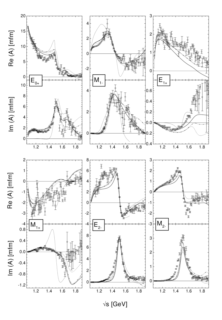
FIG. 1.: Results for the proton multipoles of pion photoproduction together with the data from SP97 [7]. Shown are all three fits: ($\cdot\!\cdot\!\cdot$) SM95-pt-1, (  $\cdot\cdot$) SM95-pt-2, ( ) SM95-pt-3. For comparison we also show the results of a $T$-matrix calculation [22] (    ).

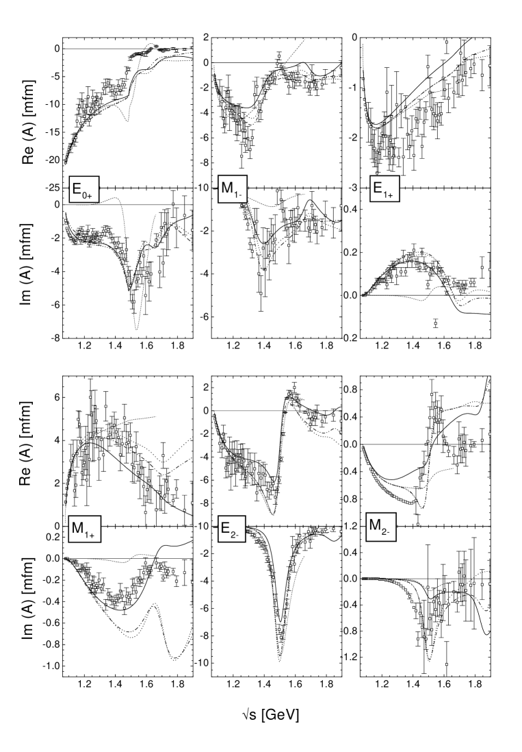
FIG. 2.: Same as Fig. 1, but for the neutron multipoles.

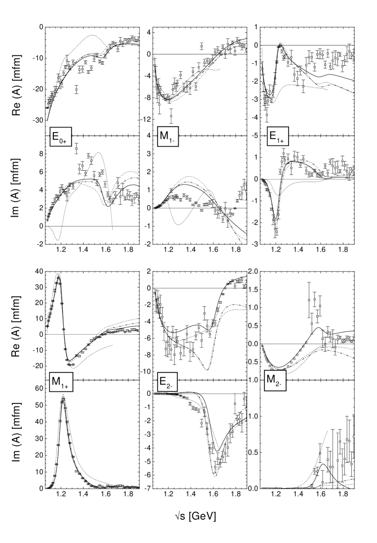
FIG. 3.: Same as Fig. 1, but for the $I\!=\!\frac{3}{2}$ multipoles.

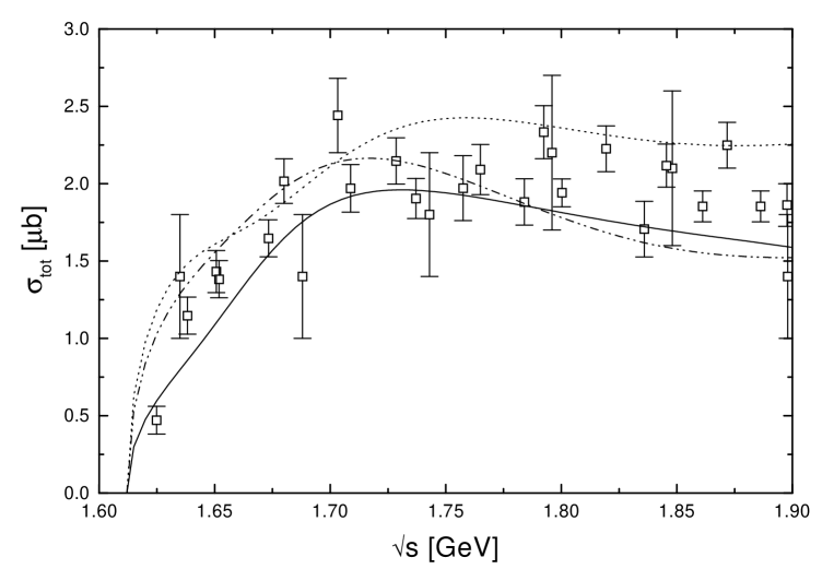
FIG. 4.: Results for the total $\gamma p\to\eta p$ (upper plot) and $\gamma p\to K^{+}\Lambda$ (lower) cross sections as compared to data from [35, 40]. In the case of eta photoproduction the reduced cross section is shown. The linecodes are those of Fig. 1.

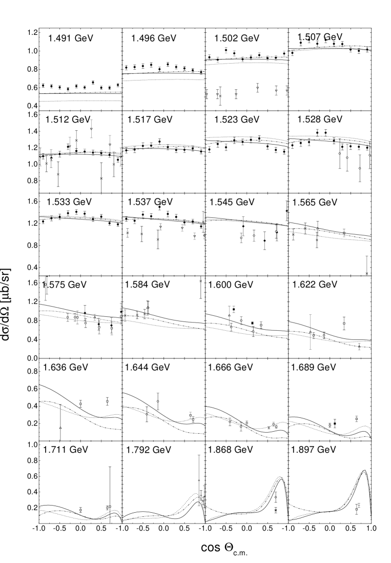
FIG. 5.: Comparison with data for the calculated differential $\gamma p\to\eta p$ cross sections at different energies. The datapoints are taken from: [34] ($\bullet$), [35], the linecodes are those of Fig. 1.

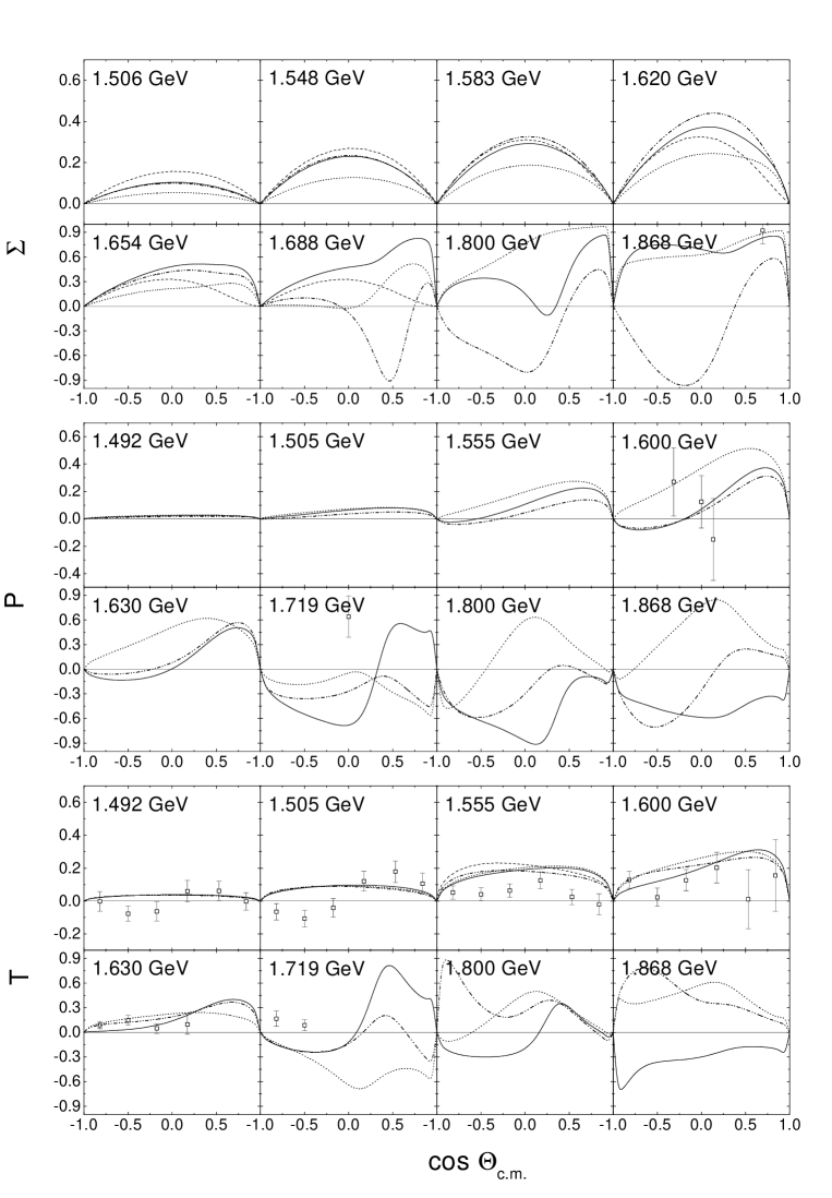
FIG. 6.: Polarization observables $\Sigma$, ${\cal P}$ and ${\cal T}$ for $\gamma p\to\eta p$ as compared to the data for different energies. For the photon asymmetry $\Sigma$ also the calculation of Knöchlein et al. [43] is shown (    ). The datapoints are taken from [35, 38], the linecodes are those of Fig. 1.

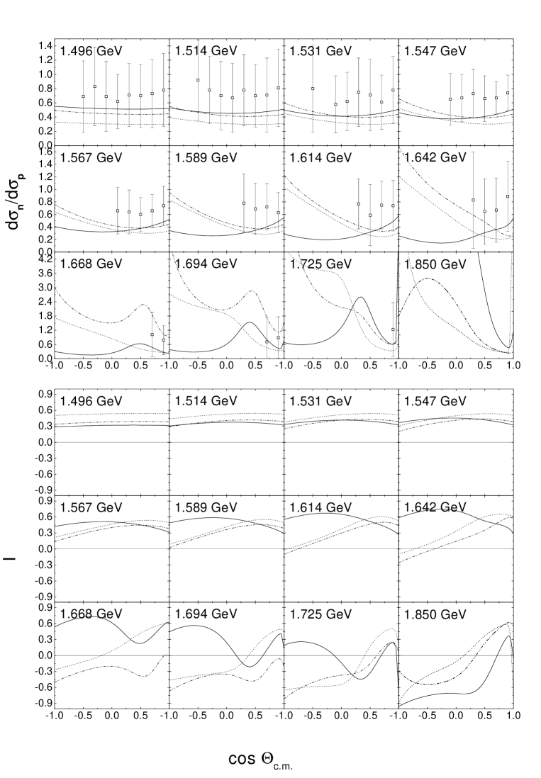
FIG. 7.: Neutron/Proton ratios and the isospin asymmetry ${\cal I}$ for $\gamma p\to\eta p$ as compared to the data for different energies. The datapoints are taken from [37], the linecodes are those of Fig. 1.

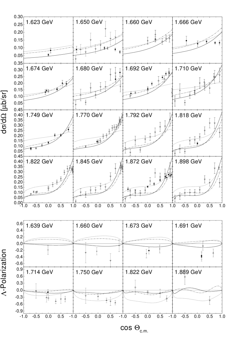
FIG. 8.: Comparison with data for the calculated differential $\gamma p\to K^{+}\Lambda$ cross sections and $\Lambda$-polarizations for different energies. The datapoints are taken from: [39] ($\Box$), [40], the linecodes are those of Fig. 1.

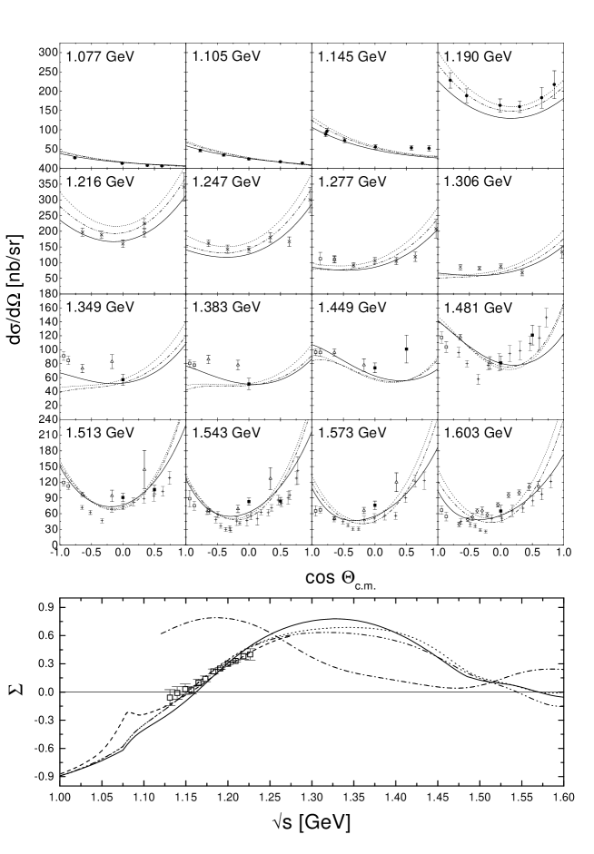
FIG. 9.: Comparison with data from [31, 32] for the calculated $\gamma p\to\gamma p$ differential cross sections (top) and photon asymmetries (bottom). The linecodes are those of Fig. 1. Also shown are the result of the isobar-model of Wada et al. [31] (  $\cdot$) and the dispersion relation calculation from L’vov [42] (    ).

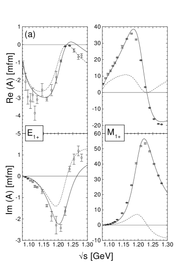
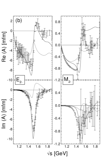
FIG. 10.: Influence of the rescattering on some of the multipoles. Shown are the results for the fit with fixed hadronic parameters with ( ) and without (    ) direct resonance coupling. (a): $P_{33}(1232)$ and $E_{1+}^{3/2}$- and $M_{1+}^{3/2}$-multipoles. (b): $D_{13}(1520)$ and $E_{2-}^{n}$- and $M_{2-}^{n}$-multipoles.

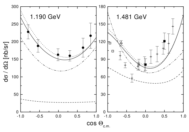
FIG. 11.: Comparison of contributions to the differential $\gamma p\to\gamma p$ cross section (data from [31]). Full calculation using SM95-pt-2 ( ), without the $\pi^{0}$ and $\eta$ contributions in the $t$-channel ($\cdot\!\cdot\!\cdot$), Born $s$- und $u$-channel diagrams only (    ). Left: $P_{33}(1232)$ contributions only (  $\cdot\cdot$). Right: $D_{13}(1520)$ contribution only (  $\cdot\cdot$).

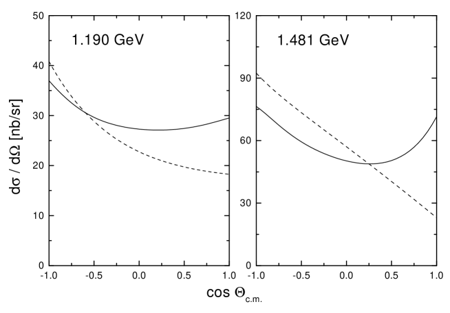
FIG. 12.: Influence of the rescattering on the nucleon $s$- and $u$-channel contributions to Compton scattering. Shown are the differential cross sections for two energies for the $K$-matrix calculation ( ) and using the $T$-matrix approximation (    ).

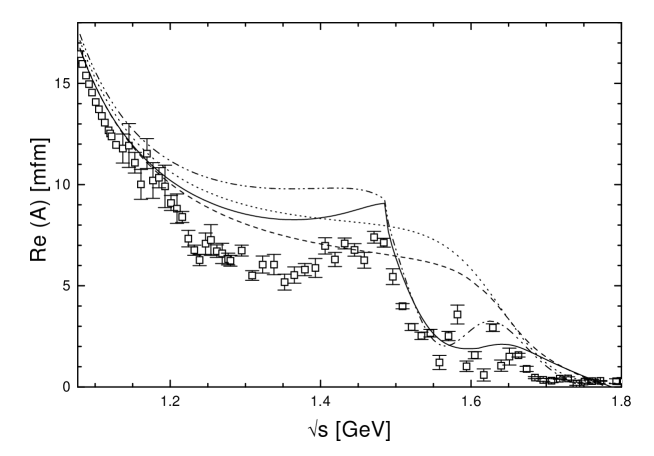
FIG. 13.: Different contributions to ${\rm Re}(E_{0+}^{p})$. Full calculation using SM95-pt-2 ( ), SM95-pt-2, but without the $S_{11}(1535)$ (    ), (  $\cdot\cdot$) and ($\cdot\!\cdot\!\cdot$) show the results of [12], both with and without the $S_{11}(1535)$.

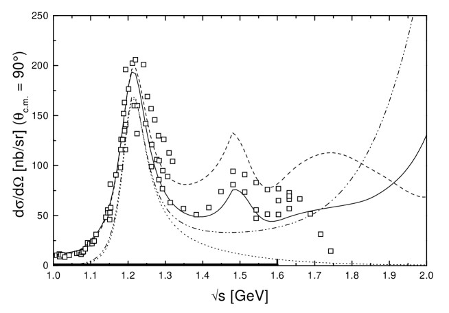
FIG. 14.: Sensitivity of the Compton cross section under 90^∘ on the helicity couplings of the $D_{13}(1520)$. Full calculation using SM95-pt-2 ( ), result using SM95-pt-2 and PDG-values for $A_{1/2,3/2}^{p}$ of the $D_{13}(1520)$ (    ) and the $P_{33}(1232)$ contribution only for $\Lambda^{e}_{3/2}$ = 4.0 GeV (  $\cdot\cdot$) and 1.1 GeV ($\cdot\!\cdot\!\cdot$). The data from [31] are shown without their errorbars. The marking on the energy axis indicates the range of data used in the fits.

REFERENCES

- [1] T. Feuster and U. Mosel, Phys. Rev. C58, 457 (1998).
- [2] R.E. Cutkosky, C.P. Forsyth, R.E. Hendrick and R.L. Kelly, Phys. Rev. D20, 2804 (1979); R.E. Cutkosky, C.P. Forsyth, J.B. Babcock, R.L. Kelly and R.E. Hendrick, Baryon 1980, Proc. 4th Int. Conf. on Baryon Resonances, ed. N. Isgur, p. 19.
- [3] E. Pietarinen, Nucl. Phys. B107, 21 (1976); R. Koch, Nucl. Phys. A448, 707 (1986) and Z. Phys. C29, 597 (1985); G. Höhler, F. Kaiser, R. Koch and E. Pietarinen, Handbook of pion-nucleon scattering, Physics Data 12-1, Karlsruhe, 1979.
- [4] B.C. Pearce and B.K. Jennings, Nucl. Phys. A528, 655 (1991).
- [5] D.M. Manley, R.A. Arndt, Y. Goradia and V.L. Teplitz, Phys. Rev. D30, 904 (1984); D.M. Manley and E.M. Saleski, Phys. Rev. D45, 4002 (1992).
- [6] Y. Surya and F. Gross, Phys. Rev. C47, 703 (1993).
- [7] SM95 and SP97 solutions of the VIRGINIA TECH PARTIAL-WAVE ANALYSIS, available via WWW from http://clsaid.phys.vt.eduCAPS. For further reference see, for example, R.A. Arndt, I.I. Strakovsky, and R.L. Workman, Phys. Rev. C53, 430 (1996) (SP97); R.A. Arndt, I.I. Strakovsky, R.L. Workman and M.M. Pavan, Phys. Rev. C52, 2120 (1995) (SM95).
- [8] S.A. Dytman, T.P. Vrana and T.-S.H. Lee, Proc. fourth CEBAF/INT Workshop on N* Physics, World Scientific, Singapore 1997 (nucl-th@xxx.lanl.gov preprint #9702033).
- [9] S. Nozawa, B. Blankleider and T.-S.H. Lee, Nucl. Phys. A513, 459 (1990); S. Nozawa and T.-S.H. Lee, Nucl. Phys. A513, 511 (1990).
- [10] R. Davidson, N.C. Mukhopadhyay and R. Wittman, Phys. Rev. D43, 71 (1991).
- [11] M. Benmerrouche, N.C. Mukhopadhyay and J.-F. Zhang, Phys. Rev. D51, 3237 (1995).
- [12] C. Sauermann, Ph.D. thesis, Darmstadt 1996; C. Deutsch-Sauermann, B. Friman and W. Noerenberg, Phys. Lett. B409, 51 (1997).
- [13] Y. Surya and F. Gross, Phys. Rev. C53, 2422 (1996).
- [14] T. Sato and T.-S.H. Lee, Phys. Rev. C54, 2660 (1996).
- [15] O. Scholten, A.Yu. Korchin, V. Pascalutsa and D. Van Neck, Phys. Lett. B384, 13 (1996).
- [16] M.L. Goldberger and K.M. Watson, Collision Theory, Wiley, New York, 1964.
- [17] Particle Data Group, Phys. Rev. D54, 1 (1996).
- [18] M. Batinić, I. Dadić, I. Šlaus, A. Švarc, B.M.K. Nefkens and T.-S.H. Lee, nucl-th@xxx.lanl.gov preprint #9703023; M. Batinić, I. Dadić, I. Šlaus, A. Švarc and B.M.K. Nefkens Phys. Rev. C51, 2310 (1995).
- [19] L.M. Nath and B.K. Bhattacharyya, Z. Phys. C5, 9 (1980).
- [20] P. van Nieuwenhuizen, Phys. Rep. 68, 228 (1981).
- [21] M. Benmerrouche and N.C. Mukhopadhyay, Phys. Rev. D46, 101 (1992).
- [22] T. Feuster and U. Mosel, Nucl. Phys. A612, 375 (1997).
- [23] R.A. Adelseck and B. Saghai, Phys. Rev. C42, 108 (1990).
- [24] M. Warns et al., Z. Phys. C45, 627 (1990).
- [25] G. Penner, Diploma thesis, Gießen 1997 and to be published.
- [26] K. Ohta, Phys. Rev. C40, 1335 (1989).
- [27] H. Haberzettl, Phys. Rev. C56, 2041 (1997); H. Haberzettl, C. Bennhold, T. Mart and T. Feuster, Phys. Rev. C58, 40 (1998).
- [28] S.I. Nagorny et al., Sov. J. Nucl. Phys. 49, 465 (1989); Sov. J. Nucl. Phys. 53, 228 (1991).
- [29] L. Tiator, C. Bennhold and S.S. Kamalov, Nucl. Phys. A580, 455 (1994).
- [30] C. Bennhold, T. Mart and D. Kusno, Proc. fourth CEBAF/INT Workshop on N* Physics, World Scientific, Singapore 1997 (nucl-th@xxx.lanl.gov preprint #9703004).
- [31] Data for the reaction : D.S. Baranov et al., Sov. J. Nucl. Phys. 21, 355 (1975); H. Genzel et al., Z. Phys. A279, 399 (1976); K. Toshioka et al., Nucl. Phys. B141, 364 (1978); M. Jung et al., Z. Phys. C10, 197 (1981); J. Duda et al., Z. Phys. C17, 1319 (1983); Y. Wada et al., Nucl. Phys. B247, 313 (1984); T. Ishii et al., Nucl. Phys. B254, 458 (1985); E.L. Hallin et al., Phys. Rev. C48, 1497 (1993); B.E. MacGibbon et al., Phys. Rev. C52, 2097 (1995); C. Molinari et al., Phys. Lett. B371, 181 (1996).
- [32] G. Blanpied et al., Phys. Rev. Lett. 76, 1023 (1996).
- [33] O. Hanstein et al., Nucl. Phys. A632, 561 (1998).
- [34] B. Krusche et al., Phys. Rev. Lett. 74, 3736 (1995); Phys. Rev. Lett. 75, 3023 (1995); Phys. Lett. B358, 40 (1995).
- [35] Data for the reaction : C. Bacci et al., Nuovo Cim. 45A, 983 (1966); Phys. Rev. Lett. 20, 571 (1968); C.A. Heusch et al., Phys. Rev. Lett. 17, 573 (1966); E.D. Bloom et al., Phys. Rev. Lett. 21, 1102 (1968); B. Delcourt et al., Phys. Lett. 29B, 75 (1969); M. Hongoh et al., Nuovo Cim. Lett. 2, 317 (1970); H.R. Hicks et al., Phys. Rev. D7, 2614 (1973); P.S.L Booth et al., Nucl. Phys. B71, 211 (1974); E.A. Abramyan et al., Jrn. of Exp. and Theo. Phys. Lett. 25, 560 (1977); V.V. Vartapetyan et al., Sov. J. Nucl. Phys. 32, 804 (1980); S. Homma et al., Jrn. Phys. Soc. Jpn. 57, 828 (1988); S.A. Dytman et al., Phys. Rev. C51, 2710 (1995).
- [36] M. Wilhelm, Ph.D. thesis, Bonn 1993, BONN-IR-93-43.
- [37] P. Hoffmann-Rothe et al., Phys. Rev. Lett. 78, 4697 (1997) and private communication.
- [38] A. Bock, Bonn 1997, BONN-IR-97-08; A. Bock et al., Phys. Rev. Lett. 81, 534 (1998) and private communication.
- [39] R. Barth et al., nucl-th@xxx.lanl.gov preprint #9707025.
- [40] Data for the reaction : P.L. Donoho and R.L. Walker, Phys. Rev. 112, 981 (1958); H.M. Brody, Phys. Rev. 119, 1710 (1960); R.L. Anderson et al., Phys. Rev. Lett. 9, 131 (1962); C.W. Peck et al., Phys. Rev. 135, 830 (1964); S. Mori., Ph.D. thesis, Cornell University 1966; D.E. Groom and J.H. Marshall, Phys. Rev. 159, 1213 (1969); A. Bleckmann et al., Z. Phys. 239, 1 (1970); T. Fujii et al., Phys. Rev. D2, 439 (1970); H. Göing et al., Nucl. Phys. B29, 121 (1971); D. Décamp et al., Orsay Report LAL-1236, 1970; P. Feller et al., Nucl. Phys. B39, 413 (1972); R.L. Anderson, Phys. Rev. D14, 679 (1976); R. Haas et al., Nucl. Phys. B137, 261 (1978).
- [41] T.Mizutani, C. Fayard, G.-H. Lamot and B. Saghai, Phys. Rev. C58, 75 (1998).
- [42] A.I. L’vov, Sov. J. Nucl. Phys. 34, 597 (1981).
- [43] G. Knöchlein, D. Drechsel and L. Tiator, Z. Phys. A352, 327 (1995) and private communication.
- [44] L. Tiator and G. Knöchlein, nucl-th@xxx.lanl.gov preprint #9802064.
- [45] R. Brockmann and R. Machleidt, Phys. Rev. C42, 1965 (1990).
- [46] B. Krusche, N.C. Mukhopadhyay, J.-F. Zhang and M. Benmerrouche, Phys. Lett. B397, 171 (1997).
- [47] R.A. Arndt, I.I. Strakovsky and R.L. Workman, nucl-th@xxx.lanl.gov preprint #9708006.
- [48] T. Wilbois, P. Wilhelm and H. Arenhövel, Phys. Rev. C57, 295 (1998).
- [49] O. Hanstein, D. Drechsel and L. Tiator, Phys. Lett. B385, 45 (1996).
- [50] M.G. Olsson, Nucl. Phys. B78, 55 (1974); M. G. Olsson and E. T. Osypowski, Nucl. Phys. B87, 399 (1975); Phys. Rev. D17, 174 (1978); Nucl. Phys. B101, 136 (1975).
- [51] J.D. Bjorken and S.D. Drell, Relativistic Quantum Mechanics, Mc Graw-Hill, 1964.
- [52] G.F. Chew, M.L. Goldberger, F.E. Low and Y. Nambu, Phys. Rev. 106, 1345 (1957).
- [53] M. Gourdin and J. Dufour, Nuovo Cim. 27, 1410 (1963).
- [54] I. Guiaşu, C. Pomponiu and E.E. Radescu, Ann. of Phys. 114, 296 (1978).
- [55] W. Pfeil, H. Rollnik and S. Stankowski, Nucl. Phys. B73, 166 (1974).
- [56] T. Ericson and W. Weise, Pions and Nuclei, Calderon Press, Oxford, 1988.