Perturbative description of nuclear double beta decay transitions

Abstract

A consistent treatment of intrinsic and collective coordinates is applied to the calculation of matrix elements describing nuclear double beta decay transitions. The method, which was developed for the case of nuclear rotations, is adapted to include isospin and number of particles degrees of freedom. It is shown that the uncertainties found in most models, in dealing with these decay modes, are largely due to the mixing of physical and spurious effects in the treatment of isospin dependent interactions.

One can hardly overestimate the importance of the double beta decay as a process explicitly linking the physics of neutrinos with the nuclear structure [1, 2, 3]. Unfortunately, the reliability of the theoretical predictions has been hampered by unstabilities in the many-body BCS + RPA - type of treatments that have been applied during the last decade [4, 5, 6, 7]. An alternative approach based on group theoretical methods has confirmed the existence of a zero-energy state for certain values of the strength of the proton-neutron, particle-particle, effective interaction [8, 9]. The appearance of such a state has been interpreted as a signature of a phase transition [10].

Here we take an alternative point of view based on the fact that the zero-energy state is a consequence of the breakdown of the isospin symmetry implicit in the (separate) neutron and proton BCS solutions [11].

As similar to the case of deformed nuclei, the symmetry may be restored in the laboratory frame through the introduction of collective coordinates. However, as different from previous cases dealing with collective coordinates, we must use here an interaction which does not conserve isospin, in order to obtain allowed matrix elements between $T\rightarrow(T-2)$ states: a central many-body problem that must be solved in double beta decay calculations is to disentangle unphysical isospin violations introduced by the theoretical treatment from physical effects due to the interaction.

In this letter we present the formalism for the case of particles moving in a single j-shell and coupled through a monopole pairing force. The hamiltonian is not necessarily isoscalar. This simple case involves all the complications associated with the collective treatment. Moreover, the predictions may be compared with those of exact calculations [9] of nuclear double beta decay transitions of the Fermi-type.

We define the operators

$$S^{+}_{v} = \sum_{m>0}c^{+}_{vm}c^{+}_{v{\bar{m}}}\;;\;\;\;\;\;\;S^{+}_{\perp}=\sum_{m>0}(c^{+}_{pm}c^{+}_{n{\bar{m}}}+c_{nm}^{+}c^{+}_{p{\bar{m}}}),$$ (1)

$$\tau_{A} = \frac{1}{2}(\tau_{p}+\tau_{n})\;;\;\;\;\;\tau_{0}=\frac{1}{2}(\tau_{p}-\tau_{n})\;;\;\;\;\;[\tau_{\bar{1}},\tau_{1}]=\tau_{0},$$ (2)

$$T_{A} = {1\over 2}\left(T_{p}+T_{n}\right)\;;\;\;\;\;\;T_{0}={1\over 2}\left(T_{p}-T_{n}\right)\;;\;\;\;\;\;[T_{\bar{1}},T_{1}]=-T_{0},$$ (3)

$$e_{A} = e_{p}+e_{n}\;;\;\;\;\;\;e_{0}=e_{p}-e_{n}.$$ (4)

where $\tau_{v}$ and $e_{v}$ are the number operators and single-particle energies, respectively, and $v=p,n$, ${\bar{1}}=-1$. The $T_{v},T_{\pm 1}$ are the generators of collective rotations in gauge-and isospace.

The collective treatment appropriate for an isospin conserving pairing interaction was introduced in refs. [12], [13], [14]. The basic set of states associated with the collective sector may be labeled by the four quantum numbers $|T_{A};T,m,k>$, where $T_{A}$ is the total number of pairs of particles. We substitute $M,T_{0}$ (the isospin projections in the laboratory and intrinsic frames) by the quantum numbers $m\equiv\frac{1}{2}(T+M)$ and $k\equiv\frac{1}{2}(T+T_{0})$, respectively. We focus on states such that $m<<T$ and $k=0$. Hereof we drop the labels $T_{A},k$ from the collective states.

The introduction of collective degrees of freedom is compensated through the appearance of the constraints

$$\tau_{z}-T_{z}=0\;;\;\;\;\;\;\;(z=n,p,\pm 1),$$ (5)

which express the fact that we can rotate the intrinsic system in one direction or the body in the opposite one without altering the physical situation [15]. Physical states should be annihilated by the four constraints and physical operators should commute with them.

Unphysical violations of the isospin symmetry take place in the intrinsic frame, which may be defined, for instance, by the condition ${\bar{S}}_{\perp}=0$, where the bar denotes the g.s. expectation value. This condition is precisely satisfied by performing a separate Bogoliubov transformation for protons and neutrons.

Physical isotensor operators have to be transformed from the laboratory frame to the intrinsic frame. In the case of the single-particle and pairing hamiltonians we have

$$H^{(lab)}_{sp} = e_{A}\tau_{A}+e_{0}(D^{1}_{00}\tau_{0}+D^{1}_{01}\tau_{1}+D^{1}_{0{\bar{1}}}\tau_{\bar{1}})$$ (6)

$$\approx e_{A}\tau_{A}+e_{0}(\tau_{0}+d^{+}d+\frac{1}{T}\tau_{1}\tau_{\bar{1}})$$ (7)

$$H^{(lab)}_{p,0} = -g_{0}(S^{+}_{p}S_{p}+S^{+}_{n}S_{n}+\frac{1}{2}S^{+}_{\perp}S_{\perp})$$ (8)

$$\approx -g_{0}(S^{+}_{p}S_{p}+S^{+}_{n}S_{n})$$ (10)

$$+\frac{g_{0}}{T^{2}}[{\bar{S}}_{n}{\bar{S}}_{p}(\tau^{2}_{1}+\tau^{2}_{\bar{1}})+({\bar{S}}^{2}_{n}+{\bar{S}}^{2}_{p})\tau_{1}\tau_{\bar{1}}]$$

$$H^{(lab)}_{p,1} = -g_{1}[D^{1}_{00}(S^{+}_{p}S_{p}-S^{+}_{n}S_{n})$$ (12)

$$\!\!\!\!\!\!-\frac{D^{1}_{01}}{\sqrt{2}}(S^{+}_{p}S_{\perp}+S^{+}_{\perp}S_{n})\,+\,\frac{D^{1}_{0{\bar{1}}}}{\sqrt{2}}(S^{+}_{n}S_{\perp}+S^{+}_{\perp}S_{p})]$$

$$\approx -g_{1}(S^{+}_{p}S_{p}-S^{+}_{n}S_{n})$$ (14)

$$+\frac{g_{1}}{T}({\bar{S}}_{p}^{2}-{\bar{S}}_{n}^{2})(d^{+}d+\frac{1}{T}\tau_{1}\tau_{\bar{1}}),$$

$$H^{(lab)}_{p,2} = -g_{2}\{D^{2}_{00}(S^{+}_{p}S_{p}+S^{+}_{n}S_{n}-S^{+}_{\perp}S_{\perp})$$ (17)

$$\!\!\!\!\!\!\!\!\!\!\!\!-\sqrt{\frac{3}{2}}[D^{2}_{01}(S^{+}_{\perp}S_{n}-S^{+}_{p}S_{\perp})+D^{2}_{0{\bar{1}}}(S^{+}_{\perp}S_{p}-S^{+}_{n}S_{\perp})]$$

$$+\sqrt{6}(D^{2}_{02}S^{+}_{p}S_{n}+D^{2}_{0{\bar{2}}}S^{+}_{n}S_{p})\}$$

$$\!\!\!\!\!\!\!\!\!\approx \!\!\!\!\!\!\!-g_{2}[(S_{p}^{+}S_{p}+S^{+}_{n}S_{n})+\frac{3}{T}{\bar{S}}_{n}{\bar{S}}_{p}(\beta^{-4}d^{2}+\beta^{4}d^{+2})$$ (19)

$$\!\!\!\!\!\!\!\!\!\!\!\!-({\bar{S}}^{2}_{p}+{\bar{S}}^{2}_{n})(\frac{3}{T}d^{+}d+\frac{1}{T^{2}}\tau_{1}\tau_{\bar{1}})-\frac{1}{T^{2}}{\bar{S}}_{n}{\bar{S}}_{p}(\tau_{1}^{2}+\tau_{\bar{1}}^{2})],$$

plus null terms which are proportional to the constraints (5). We have kept only the lowest order terms in an expansion in powers of $T^{-1}$, assuming $O({\bar{S}}_{v})=T$ and $O(g_{\nu})=T^{-1}$. Use has been made of the relation $S^{+}_{\perp}$ $\approx$ $-\frac{\sqrt{2}}{T}({\bar{S}}_{n}\tau_{1}+{\bar{S}}_{p}\tau_{\bar{1}})$. The $D^{\lambda}_{\mu\nu}$ have been expressed by means of Marshalek’s generalization of the Holstein-Primakoff representation [16], such that the operators $\beta,d^{+},d$ satisfy the relations $[d,d^{+}]=1$ and

$$(\beta)^{2t}|T,m> = |T+t,m>,$$ (20)

$$(d^{+})^{t}|T,m> = \sqrt{\frac{(m+t)!}{m!}}|T,m+t>.$$ (21)

It is easy to verify that the four components of the hamiltonian (7)-(17) commute with the constraints (5) and are therefore physical operators.

The contributions in (7)-(17) that are independent of the operators $\beta,d^{+},d,\tau_{\pm 1}$ add together to the two (proton-proton and neutron-neutron) pairing hamiltonians in a single j-shell, namely

$$H_{v}=e_{v}\tau_{v}-g_{v}S_{v}^{+}S_{v},$$ (22)

with interaction strengths $g_{p}=g_{0}+g_{1}+g_{2}$ and $g_{n}=g_{0}-g_{1}+g_{2}$. These hamiltonians are separately treated within the BCS approximation. Lagrange multiplier terms $-\lambda_{v}(\tau_{v}-T_{v})$ are added before solving the BCS equations. This treatment yields the independent quasi-particle energy terms $E_{v}{\nu}_{v}={\frac{1}{2}}\Omega g_{v}{\nu}_{v}$, where ${\nu}_{v}$ is the quasi-particle number operator for $v$-nucleons and $\Omega$ is half the value of the shell degeneracy. Within the RPA we may write

$$E_{p}\nu_{p}+E_{n}\nu_{n} \approx -\frac{g_{0}+g_{2}}{T^{2}}\,[{\bar{S}}_{p}{\bar{S}}_{n}(\tau^{2}_{1}+\tau^{2}_{\bar{1}})$$ (24)

$$+(T^{2}+{\bar{S}}_{n}^{2}+{\bar{S}}_{p}^{2})\tau_{1}\tau_{\bar{1}}].$$

Adding these contributions to the remaining terms in (7)-(17) (i.e., to the ones depending on the operators $\beta,d^{+},d,\tau_{\pm 1}$ ), one obtains for the proton-neutron sector of the spectrum (to leading order in $T^{-1}$)

$$H^{(lab)}_{(sp+p)} = {\bar{H}}+\omega_{d}d^{+}d+H_{2},$$ (25)

$${\bar{H}} = e_{v}{\bar{\tau}}_{v}-g_{v}{\bar{S}}^{2}_{v},$$ (26)

$$\omega_{d} = e_{0}+\frac{g_{1}}{T}({\bar{S}}_{p}^{2}-{\bar{S}}_{n}^{2})+\frac{3g_{2}}{T}({\bar{S}}^{2}_{p}+{\bar{S}}^{2}_{n}),$$ (28)

$$\!\!\!\!\!\!\!\!\!\!\!\!\!\!\!\!<T-2,m-2|H_{2}|T,m>=-\frac{3g_{2}}{T}{\bar{S}}_{p}{\bar{S}}_{n}\sqrt{m(m-1)},$$

plus null terms.

To leading order, the isospin operators in (7) - (17) and in (24) have a boson structure since $[\tau_{\bar{1}},(-\tau_{1})]\approx T$ and $\tau_{\bar{1}}$ annihilates the state with ${\bar{\tau}}_{0}=-T$. This is precisely the phonon that yields a zero frequency root for isoscalar hamiltonians within a naive RPA [9]. In the present treatment this phonon has disappeared from the final physical hamiltonian (10) to become part of the constraints (2). Nevertheless this degree of freedom must be taken into account in higher orders of the expansion in powers of $T^{-1}$, for instance through the BRST procedure [17], as applied to many-body problems in [15], and to the particular case of high angular momentum in [18].

The spectrum of the system is ordered into collective bands associated with particular values of the total number of particles and the isospin $(T\leq T_{A})$. The energy of the band head is given by the BCS expectation value ${\bar{H}}$. The different members of each band are labeled by the quantum number $m$ and are separated by the distance $\omega_{d}$, which includes the difference between the proton and the neutron single-particle energy $e_{0}$. There is an interband interaction which mixes different values of $T$ but it conserves the projection $M$ in the laboratory frame (cf. eq. (25)).

From the point of view of the expansion in powers of $T^{-1}$, the interband interaction is of the same order (O(1)) as the distance between the states that are mixed by it. Nevertheless, in the following we continue applying perturbation theory and we also request that $|g_{2}|<g_{v}$.

In the calculations that we report in this paper we assume $g_{p}=g_{n}=g$. The excitation energy $\omega_{d}$ is displayed for the cases $j=\frac{9}{2}$, $T_{A}=5$, $T=3$, $e_{0}=0.8$ MeV, $g=0.4$ MeV and $j=\frac{19}{2}$, $T_{A}=10$, $T=4$, $e_{0}=0.63$ MeV, $g=0.2$ MeV as functions of the ratio $g_{2}/g$ (upper boxes of fig. 1). We predict the exact results for $g_{2}=0$ and very satisfactory ones for the other values, in spite of the fact that for these results we have neglected the interband interaction.

The strong current that appears in the weak hamiltonian is proportional to the isospin operator

$$\beta_{-} = -\sqrt{2}\tau_{1}^{(lab)}=-\sqrt{2}(D^{1}_{11}\tau_{1}+D^{1}_{10}\tau_{0}+D^{1}_{1{\bar{1}}})$$ (29)

$$\approx \sqrt{2T}\,d^{+}\,+\,\mbox{null operator}.$$ (30)

The matrix element of double beta decay transitions, which for the present case correspond to pure Fermi transitions (cf. [9]), is proportional to the product of the two matrix elements

$$M_{1} = <T,1|\beta_{-}|T,0>\approx\sqrt{2T}$$ (31)

$$M_{2} = <(T-2),0|\beta_{-}|T,1>$$ (32)

$$\approx -\frac{2\sqrt{T}<(T-2),0|H_{2}|T,2>}{{\bar{H}}(T,2)-{\bar{H}}((T-2),0)},$$ (33)

These matrix elements are displayed in the lower boxes of fig. 1 for the same parameters as in the upper boxes. The expression for the interband matrix element in (25) does not distinguish whether the r.h.s. should be calculated for the initial or the final value of $T$, since it is valid for $T>>1$. Therefore, the effective interband matrix element has been chosen as the geometric average of the values obtained for each of the two connected bands.

Fig. 2 displays Fermi double beta decay matrix elements, corresponding to transitions from the initial to the final ground states. It has been calculated using the expression

$$M_{2v}=\frac{M_{1}M_{2}}{\omega_{d}+\Delta}$$ (34)

where the energy released $\Delta$ has been taken to be $0.5$ MeV, as in [9]. In addition to the exact and perturbative values of these matrix elements, we have included in this figure the results obtained by using some other approximations. The exact result shows the suppression of the matrix element around the point where the strength of the proton-neutron symmetry breaking interaction approaches the value of the fully symmetric interaction. This result is reproduced both in the naive QRPA and in the perturbative approach. The other approximation badly misses this cancellation. A detailed comparison between the results of exact, naive QRPA and renormalized QRPA (RQRPA) calculations can be found in [9]. It is worth to note that in the perturbative approach the corresponding sum rule (Ikeda’s sum rule) is exactly observed. This is not the case of other approaches, like in the case of the RQRPA of [19], where the sum rule is violated. One can easily understand this failure of the RQRPA approach, since it badly mixes-up terms in defining the components of the equation of motion. Similar conclusions about the validity of the RQRPA method are reported in [8]. The perturbative approach, as seen in figs. 1 and 2, not only reproduces exact results very satisfactorily but it also gives some insight about the mechanism responsible for the suppression of the matrix elements. As found in the calculations, the value of the matrix element $M_{2}$ depends critically on the strength of symmetry breaking terms of the interaction between protons and neutrons. The terms are proportional to $g_{2}$, as shown before. On the other hand, the values of $M_{1}$ are not very much dependent on this interaction. Finally, it should be observed that the point where the excitation energy vanishes and the point where the symmetry is completely restored are different (cf. fig. 1). This result, also obtained in the exact diagonalization of the full hamiltonian, cannot be reproduced by other means as shown in [9]. Further details will be presented in a longer publication, in which the extension of the formalism to include any number of non-degenerate j-shells has been performed and an isotensor isospin interaction has been included [20].

In conclusion, it is found that a correct treatment of collective effects induced by isospin dependent residual interactions in a superfluid system is feasible: physical effects due to the isospin symmetry-breaking terms in the hamiltonian are obtained even in the presence of the BCS mean field built upon separate proton and neutron pairing interactions. The definition of intrinsic and collective coordinates and their separation guarantees that the isospin symmetry is restored and that spurious contributions to the wave functions are decoupled from physical ones. Particularly, the problem of the unstabilities found in the standard proton-neutron QRPA are avoided by the explicit elimination of the zero frequency mode from the physical spectrum but keeping it in the perturbative expansion. The appearance of this mode cannot be avoided by the inclusion of higher order terms in the QRPA expansion or by any other ad-hoc renormalization procedure, like the renormalized QRPA of [19], once the BCS procedure is adopted for the separate treatment of proton and neutron pairing correlations.

The results shown in this letter are very encouraging, in spite of the fact that we have not used very large values of $T$. We shall discuss the extension of the formalism to cases such that $T<<O({\bar{S}}_{v})$ and its application to Gamow-Teller transitions in a forthcoming publication.

The authors are fellows of the CONICET, Argentina. (O.C.) acknowledges the grant PICT0079 of the ANPCYT, Argentina; (D.R.B and N.N.S), grants from Fundación Antorchas.

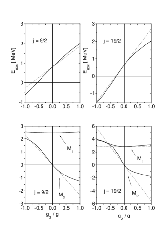
FIG. 1.: Excitation Energy and Transition Matrix Elements. Exact (solid lines) and Perturbative (dotted lines) results for the excitation energy (upper boxes) and transition matrix elements $M_{1}$ and $M_{2}$ (lower boxes) corresponding to the two different sets of parameters ($j=9/2$ and $j=19/2$) discussed in the text.

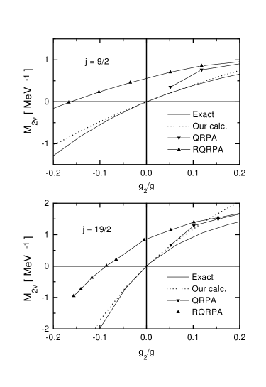
FIG. 2.: Matrix elements for Fermi double beta decay transitions calculated in several different approximations. The meaning of approximations denoted as Quasiparticle Random Phase Approximation (QRPA) and Renormalized Quasiparticle Random Phase Approximation is explained in the text. Exact and Perturbative results for the two sets of parameters utilized in the calculations are indicated by solid and dotted lines, respectively.

REFERENCES

- [1] W.C. Haxton and G.J. Stephenson, Jr., Prog. Part. Nucl. Phys. 12, 409 (1984).
- [2] F. Bohm and P.Vogel, Physics of Massive Neutrinos, Cambridge University Press, 2nd edition, Cambridge 1992.
- [3] M.Moe and P.Vogel, Ann. Rev. of Nucl. Part. Sci. 44, 247 (1994).
- [4] P. Vogel and P. Fisher, Phys. Rev. C 32, 1362 (1985).
- [5] P. Vogel and M.R. Zirnbauer, Phys. Rev. Lett. C 57, 3143 (1986).
- [6] O. Civitarese, A. Faessler and T. Tomoda, Phys. Lett. B 194, 11 (1987).
- [7] J. Suhonen and O. Civitarese, Phys. Rep. (1998) (in press).
- [8] J. Engel, S. Pittel, M. Stoitsov, P. Vogel, J. Dukelsky, Phys. Rev. C 55, 1781 (1997).
- [9] J. Hirsch, P.O. Hess and O. Civitarese, Phys. Rev. C 56, 199 (1997).
- [10] O. Civitarese, P.O. Hess and J. Hirsch, Phys. Lett. B 412, 1 (1997).
- [11] A. Bohr and B.R. Mottelson. Nuclear Structure, vol II. (Benjamin, Massachusetts, 1975)
- [12] A. Bohr, Int. Symp. on Nucl. Struc., Dubna, USSR (IAEA, Vienna, 1969).
- [13] J. Ginocchio and J.Weneser, Phys. Rev. 170, 859 (1968).
- [14] G.G. Dussel et al, Nucl. Phys. A 175, 513 (1971); G.G. Dussel, R.P.J. Perazzo and D.R. Bes, Nucl. Phys. A 183, 298 (1972); D.R. Bes et al, Nucl. Phys. A 217, 93 (1973).
- [15] D.R. Bes and J. Kurchan, The treatment of collective coordinates in many-body systems. (World Scientific, Singapore, 1990).
- [16] E.R. Marshalek, Phys. Rev. C 11, 1426 (1975).
- [17] C. Becchi, A. Rouet and S. Stora, Phys. Lett. B 52 , 344 (1974).
- [18] J. Kurchan, D.R. Bes and S. Cruz Barrios, Nucl. Phys. A 509, 306 (1990); J. P. Garrahan and D.R. Bes, Nucl. Phys. A 573, 448 (1994).
- [19] J. Toivanen and J. Suhonen, Phys. Rev. Lett 75, 410 (1995).
- [20] D.R. Bes, O. Civitarese and N.N. Scoccola, (to be published).