Pole Term and Gauge Invariance in Deep Inelastic Scattering

Abstract

In this paper we reconcile two contradictory statements about deep inelastic scattering (DIS) in manifestly covariant theories: (i) the scattering must be gauge invariant, even in the deep inelastic limit, and (ii) the pole term (which is not gauge invariant in a covariant theory) dominates the scattering amplitude in the deep inelastic limit. An “intermediate” answer is found to be true. We show that, at all energies, the gauge dependent part of the pole term cancels the gauge dependent part of the rescattering term, so that both the pole and rescattering terms can be separately redefined in a gauge invariant fashion. The resulting, redefined pole term is then shown to dominate the scattering in the deep inelastic limit. Details are worked out for a simple example in 1+1 dimensions.

I Introduction

Deep inelastic scattering (DIS) is a very important tool for investigating the structure of hadrons[1]. It involves the interaction between an energetic lepton beam (electrons, muons, neutrinos) and the respective hadron.

DIS has been described (i) in the framework of the Quark Parton Model (QPM) using the light-cone formalism and (ii) with the aid of covariant field theories. The QPM is based on the assumption that all quarks (before and after scattering) are on-shell [2]. In this manner gauge invariance is built-in. The leading contribution is the pole (or Born) term and the rescattering term is negligable in the deep inelastic limit. In descriptions based on covariant field theory, however, the intermediate quarks (or nucleons in studies of the deuteron[3]) are off-shell, and hence the pole term cannot, by itself, be gauge invariant. In this case it would appear that the pole term cannot be the leading term in the deep inelastic limit, and this has been a problem for covariant theories for many years.

To avoid this problem, de Forest [4] replaced the current by its gauge invariant part. He presented no proof, and the “de Forest prescription” has always seemed adhoc. The problem continues to trouble calculations which rely on the use of off-shell particles and dominance of the pole term. In a recent paper Kelly [5] outlines three alternatives. Assuming that the photon has four momentum $q^{\mu}=(\nu,0,0,q)$, these three alternatives can be summarized as follows:

• de Forest prescription: leave the time component of the current (the charge) unchanged, and replace the third component by $J^{3}\to(\nu/q)J^{0}$.

• Weyl prescription: leave the third component of the current unchanged, and replace the time component by $J^{0}\to(q/\nu)J^{3}$.

• Landau prescription: replace the four current by $J^{\mu}\to J^{\mu}+(J\cdot q/Q^{2})\;q^{\mu}$,

where we use the SLAC convention that $Q^{2}=-q^{2}>0$ for electron scattering. Note that each of these descriptions gives a different result for the charge and $J^{3}$ components. In the generalized Breit frame, where $q^{\mu}=(0,0,0,Q)$, the de Forest and the Landau prescriptions are identical. One of the major conclusions of this paper is a detailed theoretical argument justifying the Landau prescription.

In addition to this, we present a simple toy model for the structure functions of a composite system. The structure functions we obtain from this model exhibit scaling, are dominated in the deep inelastic limit by the “gauge invariant part” of the pole term, and give a simple, qualitative description of the distribution function of valence quarks. We present the results from two versions. In one, the particles are taken to be scalars, and the scalar “nucleon” is a bound state of a scalar “quark” with unit charge and a scalar diquark with no charge. In a second, more realistic model, the composite spin 1/2 nucleon is a bound state of a spin 1/2 quark and a scalar diquark. Stimulated by the success of QCD in 1+1 dimensions[6], we carry out these model calculations in 1+1 dimensions, obtaining finite results without the need for model dependent form factors. The only parameters in the model are the masses of the quark and diquark, $m_{1}$ and $m_{2}$ respectively. The 1+1 dimensional calculations do not necessarily give the right physics, but help in developing the necessary tools for a more complete treatment.

The remainder of this paper is divided into five sections. First we present our simple bound state model for the nuclon (which could also be applied to the description of mesons). Then we study gauge invariance and show how to uniquely define the gauge invariant part of the pole term. In Sec. IV we show for scalar quarks that the gauge invariant part of the pole term does indeed dominate DIS. The model deep inelastic structure functions are calculated and compared with experiment in Sec. V, and conclusions are given in Sec. VI.

II Bound State Equation for the “Nucleon”

We begin the discussion by constructing a dynamical model for the nucleon. In the first subsection we will assume that the scalar “nucleon” is a bound state of the two “fundamental” scalar particles: a charged “quark” $q$ of mass $m_{1}$ and an uncharged “diquark” $d$ of mass $m_{2}$. In the second subsection we will generalize to a charged spin 1/2 quark and a charged spin 1/2 nucleon.

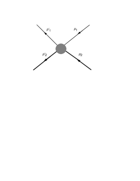
FIG. 1.: Elementary $qd$ interaction.

A Scalar ”nucleons” as bound states of scalar constituents

The two ”fundamental” constituents will interact with each other via the coupling shown in Fig. 1:

$$V=\lambda f(p^{2}_{2})f(p^{\prime 2}_{2})$$ (1)

where $\lambda$ is the coupling strength, and the form factor $f(p_{2}^{2})$ is a function of the square of the diquark four-momentum. For generality, we keep these form factors for now, but they will be set to unity later when we carry out calculations in 1+1 dimensions. Hence the scattering amplitude is:

$${\cal M}=\lambda f(p^{2}_{2})f(p^{\prime 2}_{2})+(-i)^{4}\lambda^{2}f(p^{2}_{2})f(p^{\prime 2}_{2})\,b(s)+...=\frac{\lambda f(p^{2}_{2})f(p^{\prime 2}_{2})}{1-\lambda\,b(s)};$$ (2)

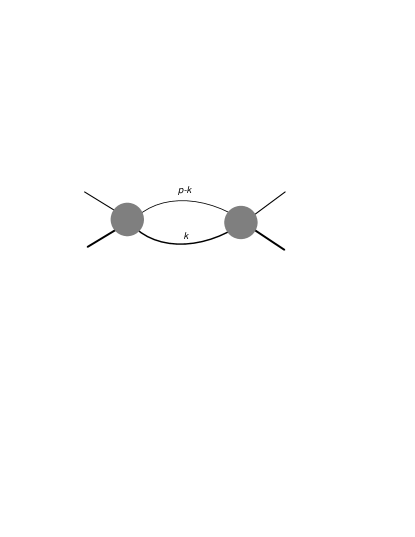
FIG. 2.: The bubble diagram.

where we have introduced the function $b(s)$ defined by

$$b(s)=i\int{\frac{d^{d}k}{(2\pi)^{d}}\frac{f^{2}(k^{2})}{(m_{2}^{2}-k^{2}-i\epsilon)(m_{1}^{2}-(p-k)^{2}-i\epsilon)}}\,,$$ (3)

with $p=p_{1}+p_{2}$ and $s=p^{2}$. This “bubble” integral is represented graphically in Fig. 2. The mass of the bound state must be below threshold, and for simplicity we assume $m_{2}-m_{1}<M<m_{1}+m_{2}$.

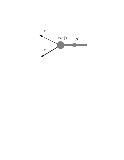
FIG. 3.: The “nucleon”$qd$ vertex.

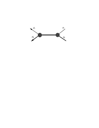
FIG. 4.: The dressed bound state pole contribution to the $qd$ scattering amplitude.

In this simple separable model, the bound state is described by the “nucleon”$qd$ vertex function

$$\Gamma(p_{2})={\cal N}f(p_{2}^{2})\,,$$ (4)

where ${\cal N}$ is a constant to be determined from the normalization of the wave function. This is shown in Fig. 3. Denoting the dressed propagator of the bound nucleon by $\Delta_{B}(p)$, the dressed $qd$ scattering amplitude is given exactly in this simple model by

$${\cal M}=-\Gamma(p_{2})\Delta_{B}(p)\Gamma(p^{\prime}_{2})\,,$$ (5)

where

$$-{\cal N}^{2}\Delta_{B}(p)=\frac{\lambda}{1-\lambda\,b(s)}\,.$$ (6)

Eq. (5) is illustrated in Fig. 4.

Since the propagator should have a pole at $s=M^{2}$, it is useful to expand the bubble $b(s)$ in this vicinity, so the denominator of the RHS of Eq. (6) is

$$1-\lambda b(M^{2})+\lambda(M^{2}-s)\,b^{\prime}(M^{2})+\cdots$$

and this must vanish at $s=M^{2}$. Consequently $\lambda b(M^{2})=1$ is a necessary condition of the bound state, and near the pole Eq. (6) becomes

$$-{\cal N}^{2}\Delta_{B}(p)=\frac{1}{(M^{2}-s)\,b^{\prime}(M^{2})+\cdots}.$$ (7)

Knowing that, in the vicinity of $s=M^{2}$, the nucleon propagator should be

$$\Delta_{B}(p)\simeq\frac{1}{M^{2}-s-i\epsilon}\,,$$ (8)

allows us to find the normalization of the $Nqd$ vertex function:

$${\cal N}=\sqrt{\frac{-1}{b^{\prime}(M^{2})}}\,.$$ (9)

Note that the existance of the bound state implies that $b^{\prime}(M^{2})<0$, which will be shown below.

In 1+1 D the bubble integral will converge without form factors, and we can assume, for simplicity, that $f(p^{2}_{2})\equiv 1$. The bubble integral (3) is then model independent, and easily calculated. If it is parametrized using Feynman variables, one can either compute the loop below treshold directly in Minkowski space (doing the momentum integration first and then integrating over the Feynman variable) or compute it in Euclidian space and Wick rotate back to the Minkowski space. Introducing the triangle function

$$\Delta(p^{2},m_{1}^{2},m_{2}^{2})=(p^{2}-m_{1}^{2}-m_{2}^{2})^{2}-4m_{1}^{2}m_{2}^{2}\,,$$ (10)

which is negative if $(m_{2}-m_{1})^{2}<p^{2}<(m_{2}+m_{1})^{2}$, the bubble becomes:

$$b(s)=-\frac{1}{2\pi}\frac{1}{\sqrt{-\Delta(s,m_{1}^{2},m_{2}^{2})}}\;\arctan\left[\frac{\sqrt{-\Delta(s,m_{1}^{2},m_{2}^{2})}}{s-m_{1}^{2}-m_{2}^{2}}\right]\,.$$ (11)

This is real, and if the mass of the bound state is to be $M$, then $\lambda$ must be

$$\lambda=-2\pi\sqrt{-\Delta(M^{2},m_{1}^{2},m_{2}^{2})}\left[\arctan\left(\frac{\sqrt{-\Delta(M^{2},m_{1}^{2},m_{2}^{2})}}{M^{2}-m_{1}^{2}-m_{2}^{2}}\right)\right]^{-1}\,.$$ (12)

This is real (so the Lagrangian is hermitian, as it should be) and negative (as expected from the fact that we have a bound state, implying the interaction is attractive). In fact, the whole 1+1 D theory can be derived from the Lagrangian

$${\cal L}=\frac{1}{2}(\partial^{\mu}d)(\partial_{\mu}d)-\frac{1}{2}m_{2}^{2}d^{2}+(\partial^{\mu}q)(\partial_{\mu}q)^{\dagger}-m_{1}^{2}qq^{\dagger}-\frac{\lambda}{2}d^{2}qq^{\dagger},$$ (13)

where $q$ is the “quark” and $d$ the “diquark” fields. From this Lagrangian, or from Eq. (1), one sees that $\lambda$ must be negative in order for a bound state to exist.

Above threshold, however, the loop $b(s)$ also has an imaginary part

$$\Im b(s)=\frac{-1}{2\sqrt{\Delta(s,m_{1}^{2},m_{2}^{2})}}\,,$$ (14)

which can be calculated in two ways. The first method is a computation based on Cutkosky’s rules, which are easily handled in this simple case. The second follows directly from the Feynman parametrization of Eq. (3). Integrating over the internal momentum gives

$$b(s)=-\frac{1}{4\pi}\int^{1}_{0}\frac{dx}{m_{1}^{2}x+m_{2}^{2}(1-x)-s\,x(1-x)-i\epsilon}\,.$$ (15)

Introducing the variable $s^{\prime}={m_{2}^{2}}/{x}+{m_{1}^{2}}/({1-x})$ transforms (15) into:

$$b(s)=-\frac{1}{\pi}\int^{\infty}_{(m_{1}+m_{2})^{2}}\frac{ds^{\prime}}{s^{\prime}-s-i\epsilon}\;\left[\frac{1}{2\sqrt{\Delta(s^{\prime},m_{1}^{2},m_{2}^{2})}}\right]\,.$$ (16)

This expression yields a real value for $b(s)$ if $s$ is below threshold because $\Delta(s^{\prime},m_{1}^{2},m_{2}^{2})$ is positive above threshold. This relation is a dispersion relation, and comparing it with the general form

$$f(s)=\frac{1}{\pi}\int^{\infty}_{\rm treshold}{\frac{ds^{\prime}\,\Im f(s^{\prime})}{s^{\prime}-s-i\epsilon}}\,,$$ (17)

one concludes that the imaginary part of the bubble is correctly given in Eq. (14). As a byproduct, we have also discovered the correct phase space factor for use with dispersion relations in 1+1 D.

The real part of $b(s)$ above treshold can also be found in two ways: (i) using Eq. (17), or (ii) by analytically continuing Eq. (11), a procedure which also provides a third method for computing the bubble’s imaginary part. As a result of these calculations, the real part above treshold is found to be:

$$\Re b(s)=\frac{-1}{4\pi\sqrt{\Delta(s,m_{1}^{2},m_{2}^{2})}}\ln\left[\frac{s^{2}-s(m_{1}^{2}+m_{2}^{2})+s\sqrt{\Delta(s,m_{1}^{2},m_{2}^{2})}}{s^{2}-s(m_{1}^{2}+m_{2}^{2})-s\sqrt{\Delta(s,m_{1}^{2},m_{2}^{2})}}\right]\,.$$ (18)

At large $s$, $\Im b(s)\sim s^{-1}$, $\Re b(s)\sim s^{-1}\ln({s}/{m_{2}^{2}})$; so $b(s)\rightarrow 0$ as $s\rightarrow\infty$. This important result will be used below.

Before turning to the spin 1/2 case, we use the representation (15) to write the normalization condition (9) in the following form:

$$1=\frac{{\cal N}^{2}}{4\pi}\int^{1}_{0}dx\frac{x(1-x)}{\left[m_{1}^{2}x+m_{2}^{2}(1-x)-M^{2}\,x(1-x)\right]^{2}}\,.$$ (19)

This relation will be used again in the following sections.

B Generalization to spin 1/2 nucleons and quarks

In this subsection we will repeat our former calculations for the more realistic case of charged spin 1/2 nucleons and quarks (retaining, however, the uncharged scalar diquark). The quark-diquark contact interaction is assumed to be a scalar in the Dirac space of the quarks, with the momentum space dependence previously given in Eq.  (1).

In this case the bubble in $d$ dimensions becomes:

$$b(p)=i\int\frac{d^{d}k}{(2\pi)^{d}}\frac{f^{2}(k^{2})}{(m_{2}^{2}-k^{2}-i\epsilon)(m_{1}-(\not p-\not k)-i\epsilon)},$$ (20)

or, after the integration:

$$b(p)=A(p^{2})+B(p^{2})\not p.$$ (21)

In 1+1 dimensions with the form factors set to unity, the factors $A(p^{2})$ and $B(p^{2})$ become:

$$A(p^{2})= -\frac{m_{1}}{4\pi}\int^{1}_{0}\frac{dx}{m_{1}^{2}x+m_{2}^{2}(1-x)-p^{2}x(1-x)}\$$ (22)

$$B(p^{2})= -\frac{1}{4\pi}\int_{0}^{1}\frac{(1-x)\,dx}{m_{1}^{2}x+m_{2}^{2}(1-x)-p^{2}x(1-x)}\,,$$ (23)

where $x$ is the Feynman parameter used previously in Eq. (15). In the presence of spin, Eq. (2) is modified:

$${\cal M}=\frac{\lambda\;(1-\lambda A(p^{2})+\lambda B(p^{2})\not p)}{(1-\lambda A(p^{2}))^{2}-\lambda^{2}B^{2}(p^{2})p^{2})}\,.$$ (24)

Expanding the denominator near the nucleon pole gives

$$(1-\lambda A(p^{2}))^{2}-\lambda^{2}B^{2}(p^{2})p^{2}= (1-\lambda A_{0})^{2}-2\lambda A^{\prime}(1-\lambda A_{0})(p^{2}-M^{2})$$ (26)

$$-\lambda^{2}(B_{0}^{2}+2B_{0}B^{\prime}(p^{2}-M^{2}))p^{2}+\cdots\,,$$

where $A_{0}=A(p^{2})$, $B_{0}=B(p^{2})$, the primes denote derivatives with respect of $p^{2}$, and all functions are evaluated at $p^{2}=M^{2}$. The denominator vanishes at $p^{2}=M^{2}$ if

$$1-\lambda A_{0}=M\lambda B_{0}.$$ (27)

This is the bound state condition. After imposing the bound state condition, in the vicinity of the poles the scattering amplitude becomes:

$${\cal M}\simeq\frac{M+\not p}{(M^{2}-p^{2})(B_{0}+2MA^{\prime}+2M^{2}B^{\prime})}.$$ (28)

The normalization factor ${\cal N}$ is then:

$${\cal N}^{-2}=-\left[2M(A^{\prime}+MB^{\prime})+B_{0}\right]\,.$$ (29)

Using the relations (23), and the identity

$$0=\int^{1}_{0}dx\;\frac{m_{1}^{2}x^{2}-m_{2}^{2}(1-x)^{2}}{\left[m_{1}^{2}x+m_{2}^{2}(1-x)-M^{2}x(1-x)\right]^{2}}.$$ (30)

we may rewrite the renormalization condition (29) in the following form:

$$1=\frac{{\cal N}^{2}}{4\pi}\int^{1}_{0}dx\;\frac{x(M(1-x)+m_{1})^{2}}{\left[m_{1}^{2}x+m_{2}^{2}(1-x)-M^{2}x(1-x)\right]^{2}}.$$ (31)

This relation will be needed later to verify baryon number conservation.

III Deep Inelastic Scattering and Gauge Invariance

We now add electromagnetic interactions to the model, and study the implications of the requirement that the e.m. interaction be gauge invariant. We begin by restoring the form factors; later we will move to 1+1 dimensions and set the form factors to unity. As in the previous section, we will first carry out the discussion for a scalar quark and nucleon, and later extend it to a spin 1/2 quark and nucleon.

A The scalar model

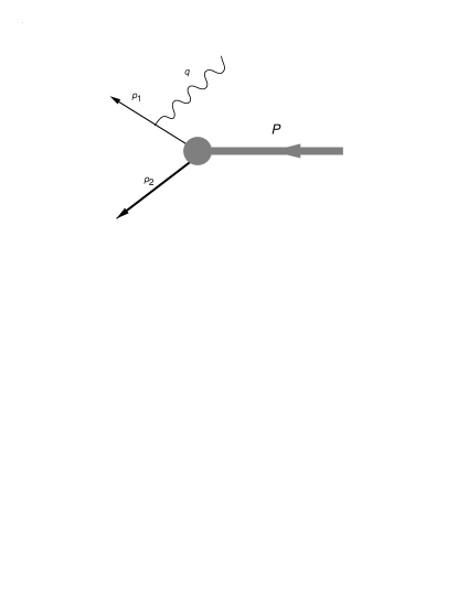
FIG. 5.: The pole term.

Start with the pole term, shown in Fig. 5, which gives

$$e{\cal J}^{\mu}_{a}=i(-i)^{3}ej^{\mu}(p_{1},p^{\prime}_{1})\Delta(p_{1}^{\prime})\Gamma(p_{2})\,,$$ (32)

where $p^{\prime}_{1}=p_{1}-q$, the propagator of the scalar (charged) “quark” is

$$\Delta(p_{1})=\frac{1}{m_{1}^{2}-p_{1}^{2}-i\epsilon}\,,$$ (33)

and $j^{\mu}(p_{1},p_{1}^{\prime})$ is the one-body current of the quark. (Note that our definition of the current ${\cal J}$ does not include the charge.) We assume that the diquark has no electromagnetic interaction, so there are no diagrams with the photon coupling to the diquark. We require that the quark current satisfy the Ward-Takahashi (WT) identity:

$$q^{\mu}j_{\mu}(p_{1},p_{1}^{\prime})=\Delta(p_{1}^{\prime})-\Delta(p_{1})\,.$$ (34)

The current of a bare, spinless particle

$$j^{\mu}(p_{1},p_{1}^{\prime})=(p_{1}+p^{\prime}_{1})^{\mu}$$ (35)

satisfies this identity.

Using the WT identity, and noting that $\Delta^{-1}(p_{1})=0$ because $p_{1}^{2}=m_{1}^{2}$, we see that the pole term by itself is not gauge invariant

$$q_{\mu}{\cal J}^{\mu}_{a}= -q_{\mu}j^{\mu}(p_{1},p_{1}^{\prime})\Delta(p_{1}^{\prime})\Gamma(p_{2})$$ (36)

$$= -\left[\Delta^{-1}(p_{1}^{\prime})-\Delta^{-1}(p_{1})\right]\,\Delta(p_{1}^{\prime})\Gamma(p_{2})$$ (37)

$$= -\Gamma(p_{2})\neq 0\,.$$ (38)

Hence the pole term by itself cannot be a good approximation for the scattering amplitude.

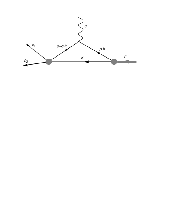
FIG. 6.: The rescattering diagram.

To obtain a gauge invariant result, it is necessary to add the rescattering term shown in Fig. 6. This term is

$$e{\cal J}_{b}^{\mu}= i(-i)^{6}e\frac{\lambda f(p_{2}^{2})}{1-\lambda b(s^{\prime})}$$ (40)

$$\times\int\frac{d^{d}k}{(2\pi)^{d}}\frac{f(k^{2})j^{\mu}(p^{\prime}-k,p-k)\Gamma(k)}{(m_{1}^{2}-(p^{\prime}-k)^{2}-i\epsilon)(m_{1}^{2}-(p-k)^{2}-i\epsilon)(m_{2}^{2}-k^{2}-i\epsilon)}\,,$$

where $p^{\prime}=p+q$ and $s^{\prime}=p^{\prime 2}$ is the square of the momentum of the final state after it has absorbed the virtual (space-like) photon. Note that $p^{2}=s=M^{2}$ but that $p^{\prime 2}=s^{\prime}\geq M^{2}$.

This diagram is also not gauge invariant. Using Eq. (4) and the WT identity gives

$$q_{\mu}{\cal J}^{\mu}_{b}=-\frac{{\cal N}f(p_{2}^{2})}{1-\lambda b(s^{\prime})}\left[\lambda b(s^{\prime})-\lambda b(M^{2})\right]={\cal N}f(p_{2}^{2})=\Gamma(p_{2})\,,$$ (41)

where the bound state condition $\lambda b(M^{2})=1$ was used in the second step. This is not gauge invariant, but if we add the rescattering term to the pole term the total amplitude is

$$q_{\mu}\left({\cal J}^{\mu}_{a}+{\cal J}^{\mu}_{b}\right)=0\,.$$ (42)

Stated in a different way, the gauge dependent parts of the pole term and the rescattering term cancel.

We now face the question posed in the introduction: How can the pole term dominate the scattering in the deep inelastic limit if it is not gauge invariant? To answer this question we break the pole term into a gauge invariant part and a gauge dependent part as follows:

$${\cal J}_{a}^{\mu}=-{(2p_{1}-q)^{\mu}\Gamma(p_{2})\over m_{1}^{2}-(p_{1}-q)^{2}}=-{\left[I_{1}^{\mu}(p_{1})+I_{2}^{\mu}(p_{1})\right]\,\Gamma(p_{2})\over m_{1}^{2}-(p_{1}-q)^{2}}\,,$$ (43)

where

$$I^{\mu}_{1}(p_{1})= 2\left(p_{1}^{\mu}-\frac{(q\cdot p_{1})}{q^{2}}q^{\mu}\right)\,,$$ (44)

$$I^{\mu}_{2}(p_{1})= -q^{\mu}\left(1-\frac{2(q\cdot p_{1})}{q^{2}}\right)=-{q^{\mu}\over q^{2}}\left[(p_{1}-q)^{2}-m_{1}^{2}\right]\,.$$ (45)

Note that $q_{\mu}I_{1}^{\mu}=0$, and that the gauge dependent part of the pole term reduces to

$${\cal J}^{\mu}_{ag}=-\frac{q^{\mu}}{q^{2}}\,\Gamma(p_{2})\,.$$ (46)

Now the rescattering term can also be similarly decomposed. Noting that

$$j^{\mu}(p^{\prime}-k,p-k)=I_{1}^{\mu}(p^{\prime}-k)+I_{2}^{\mu}(p^{\prime}-k)$$ (47)

the gauge dependent part of the rescattering term becomes

$${\cal J}^{\mu}_{bg}= -{q^{\mu}\over q^{2}}\;\frac{\lambda\Gamma(p_{2})}{[1-\lambda b(s^{\prime})]}$$ (49)

$$\times i\int\frac{d^{d}k}{(2\pi)^{d}}\frac{f^{2}(k^{2})\Bigl{\{}(p-k+q)^{2}-(p-k)^{2}\Bigr{\}}}{(m_{2}^{2}-k^{2})(m_{1}^{2}-(p-k)^{2})(m_{1}^{2}-(p-k+q)^{2})}$$

$$= {q^{\mu}\over q^{2}}\,\Gamma(p_{2})\;\frac{\lambda}{[1-\lambda b(s^{\prime})]}\Bigl{\{}b(M^{2})-b(s^{\prime})\Bigr{\}}={q^{\mu}\over q^{2}}\,\Gamma(p_{2})\,,$$ (50)

which exactly cancels the gauge dependent part of the pole term!

We have shown that, if we drop the parts from each terms, the Born pole term and the rescattering term are redefined so that each is separately gauge invariant. As it turns out, the redefined pole term is identical to the Landau prescription defined in the introduction. We have just justified this prescription.

It is clear that the same decomposition works in 1 + 1 dimensions, where the form factor $f=1$. In this case the diagrams come from from the Lagrangian (13), modified to include electromagnetic interactions. The new Lagrangian is

$${\cal L}=\frac{1}{2}(\partial^{\mu}d)(\partial_{\mu}d)-\frac{1}{2}m_{2}^{2}d^{2}+(D_{\mu}q)(D^{\mu}q)^{\dagger}-m_{1}^{2}qq^{\dagger}-\frac{\lambda}{2}d^{2}qq^{\dagger}\,,$$ (51)

where the fields are the same as in the preceding section, but the gradient of the charged field has been replaced by the covariant derivative

$$D^{\mu}=\partial^{\mu}-ieA^{\mu}\,.$$ (52)

B Extension to sin 1/2 quarks and nucleons

We how extend the above results to the spin 1/2 model previously introduced. The Born term for a structureless quark (with the form factor set equal to unity) is

$$e{\cal J}^{\mu}_{a}=-ej^{\mu}(p_{1},p^{\prime}_{1})S(p_{1}^{\prime})\Gamma(p_{2},p)\,,$$ (53)

where now $j^{\mu}=\gamma^{\mu}$ and the quark propagator is

$$S(p_{1}^{\prime})={1\over m_{1}-\not p^{\prime}-i\epsilon}\,.$$ (54)

The vertex function for the spin 1/2 case is

$$\Gamma(p,\lambda_{N})={\cal N}{U}_{N}(p,\lambda_{N})$$ (55)

where $\lambda_{N}$ is the helicity of the nucleon and ${U}_{N}(p,\lambda_{N})$ are the helicity spinor of the nucleon. Using the Dirac equation for the final quark, the pole term can be written

$${\cal J}^{\mu}=-\frac{{\cal N}}{m_{1}^{2}-(p_{1}-q)^{2}}\;{\bar{u}}(p_{1},\lambda_{1})\left[2p_{1}^{\mu}-\gamma^{\mu}\not q\right]{U}_{N}(p,\lambda_{N}),$$ (56)

where $\lambda_{1}$ the helicity of the outgoing quark and $u(p_{1},\lambda_{1})$ the helicity spinor of the quark. Now the current is spin dependent.

As before, we decompose the pole term into a gauge invariant and gauge noninvariant part:

$${\cal J}^{\mu}_{a}= -\frac{{\cal N}}{m_{1}^{2}-(p_{1}-q)^{2}}\;{\bar{u}}(p_{1},\lambda_{1})\left[2p_{1}^{\mu}-\frac{2p_{1}\cdot qq^{\mu}}{q^{2}}-\gamma^{\mu}\not q+q^{\mu}\right]{U}_{N}(p,\lambda_{N})$$ (57)

$${\cal J}^{\mu}_{ag}= -\frac{q^{\mu}}{q^{2}}\;{\cal N}{\bar{u}}(p_{1},\lambda_{1}){U}_{N}(p,\lambda_{N})=-\frac{q^{\mu}}{q^{2}}\;{\bar{u}}(p_{1},\lambda_{1})\Gamma(p,\lambda_{N})\,.$$ (58)

Note that, except for the addition of the spinors, the gauge dependent part identical to the scalar case, and the gauge independent part is again the Landau prescription.

We now look at the spinor rescattering diagram. Introducing the decomposition

$$j^{\mu}(p^{\prime}-k,p-k)= \gamma^{\mu}-{q^{\mu}\not q\over q^{2}}+{q^{\mu}\not q\over q^{2}}$$ (59)

$$= \gamma^{\mu}-{q^{\mu}\not q\over q^{2}}-{q^{\mu}\over q^{2}}\,\Bigl{\{}S^{-1}(p-k+q)-S^{-1}(p-k)\Bigr{\}}\,,$$ (60)

the gauge dependent part of the rescattering term becomes

$${\cal J}^{\mu}_{bg}= {q^{\mu}\over q^{2}}\;\lambda\;{\bar{u}}(p_{1},\lambda_{1})\left[1-\lambda b(p+q)\right]^{-1}$$ (63)

$$\times i\int\frac{d^{d}k}{(2\pi)^{d}}\frac{1}{(m_{2}^{2}-k^{2})}S(p-k+q)\Bigl{\{}S^{-1}(p-k+q)-S^{-1}(p-k)\Bigr{\}}$$

$$\qquad\times S(p-k)\;\Gamma(p,\lambda_{N})$$

$$= {q^{\mu}\over q^{2}}\;{\bar{u}}(p_{1},\lambda_{1})\left[1-\lambda b(p+q)\right]^{-1}\Bigl{\{}\lambda\,b(p)-\lambda\,b(p+q)\Bigr{\}}\;\Gamma(p,\lambda_{N})$$ (64)

$$= {q^{\mu}\over q^{2}}\;{\bar{u}}(p_{1},\lambda_{1})\;\Gamma(p,\lambda_{N})\,,$$ (65)

where we used the bound state condition (27) and $\not p\Gamma(p,\lambda_{N})=M\Gamma(p,\lambda_{N})$. Note that this term exactly cancels the gauge dependent part of the pole term!

This argument shows that this technique is quite general, and should work in every case. The pole term is divided into a term which is gauge invariant and one proportional to $q^{\mu}$ by adding and subtracting a (unique) term proportional to $q^{\mu}$. Then it may be shown that this non gauge invariant term is cancelled when the rescattering term is similarily separated into (unique) gauge invariant and non guage invariant parts. Knowing that this works means that the non gauge invariant part of the pole term can be discarded without checking that it is cancelled by an identical piece from the rescattering term. Our argument can be extended to currents with form factors if we use the technique developed by Gross and Riska [7] to define the off-shell currents.

IV Rescattering and The Triangle Diagram

In this section we consider the rescattering term for the scalar model in more detail. We compute it exactly for the case $q=0$ and confirm that the charge of the bound state is properly normalized. Then we study the behavior of the elastic form factor and the inelastic rescattering term at large $q^{2}$. We will compare the gauge invariant part of the rescattering term with the gauge invariant part of the pole term and show that the pole term dominates at high $q^{2}$. In order to achieve convergence in a model independent way, we return to 1+1 dimension.

The key to these calculations is the triangle diagram. The gauge invariant part of this diagram is

$$t^{\mu}(p^{\prime},p)=-{2i\over q^{2}}\int\frac{d^{2}k}{(2\pi)^{2}}\;\frac{q^{2}(p-k)^{\mu}-q^{\mu}\,q\cdot(p-k)}{(m_{2}^{2}-k^{2})(m_{1}^{2}-(p+q-k)^{2})(m_{1}^{2}-(p-k)^{2})}\,.$$ (66)

Feynman parametrizing the integral and doing the momentum integration gives

$$t^{\mu}(p^{\prime},p)=\left(p^{\mu}-{q^{\mu}\,q\cdot p\over q^{2}}\right)\;\frac{1}{8\pi}\int^{1}_{0}dx\int^{1-x}_{0}dy\;\;\frac{1-x-y}{D^{2}(x,y,p,q)}\,,$$ (67)

where the denominator is

$$D(x,y,p,q)= (px+qx+py)^{2}$$ (69)

$$+x\,\left(m_{1}^{2}-(p+q)^{2}-m_{2}^{2}\right)+y\,\left(m_{1}^{2}-p^{2}-m_{2}^{2}\right)+m_{2}^{2}\,.$$

It is convenient to express the integral in terms of $p^{\prime}=p+q$ and $p$, and to change to the variables

$$z= x+y$$ (70)

$$u= {(x-y)\over z}\,,$$ (71)

which maps the region of integration into

$$0 \leq z\leq 1$$ (72)

$$-1 \leq u\leq 1\,.$$ (73)

The Jacobian of this transformation is $z/2$, and the integral then becomes

$$t^{\mu}(p^{\prime},p)=\left\{(p^{\prime}+p)^{\mu}-{q^{\mu}\,(p^{\prime 2}-p^{2})\over q^{2}}\right\}\;\frac{1}{8\pi}\int^{1}_{0}dz\int^{1}_{-1}du\;\;\frac{z(1-z)}{d^{2}(z,u,p^{\prime},p)}\,,$$ (74)

where

$$d(z,u,p^{\prime},p)= m_{2}^{2}(1-z)+m_{1}^{2}z-{\textstyle{1\over 2}}(p^{\prime 2}+p^{2})z(1-z)$$ (76)

$$-{\textstyle{1\over 2}}(p^{\prime 2}-p^{2})uz(1-z)-{\textstyle{1\over 4}}q^{2}z^{2}(1-u^{2})\,.$$

We will use the general results (74) and (76) in the following discussion.

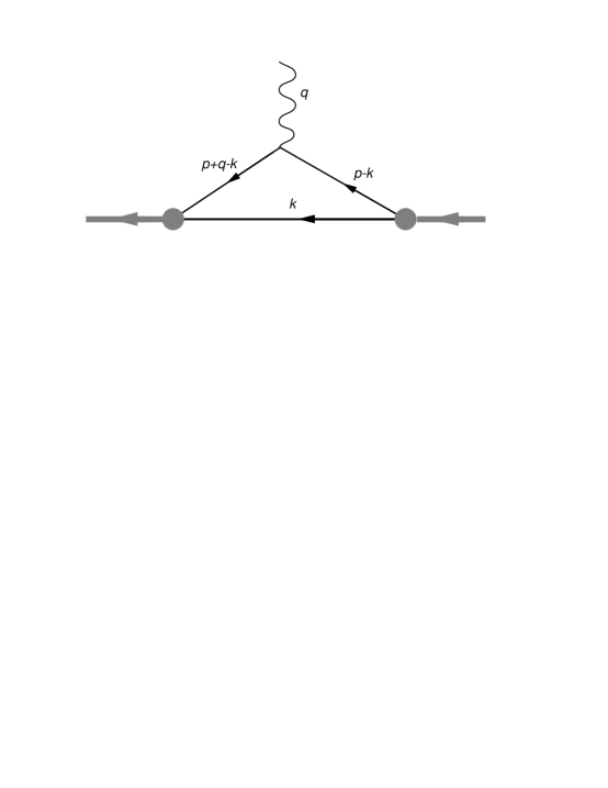
FIG. 7.: The hadronic part of the elastic electron-nucleon scattering process, proportional to the deuteron form factor.

A Charge Normalization

First consider the hadronic part of the elastic electron-nucleon scattering process, shown in Fig. 7. This diagram is gauge invariant by itself, and hence the deuteron form factor is given by

$$e{\cal J}^{\mu}_{e}=e\,F(q^{2})\,(p^{\prime}+p)^{\mu}=e\,{\cal N}^{2}\,t^{\mu}(p^{\prime},p)\,,$$ (77)

where, for elastic scattering, the triangle diagram is evaluated with the constraints $p^{\prime 2}=(p+q)^{2}=M^{2}=p^{2}$. Substituting Eq. (74) into Eq. (77) gives

$$F(q^{2})=\frac{{\cal N}^{2}}{8\pi}\int^{1}_{0}dz\int^{1}_{-1}du\;\;\frac{z(1-z)}{\left[\alpha(z)-{\textstyle{1\over 4}}q^{2}z^{2}(1-u^{2})\right]^{2}}\,,$$ (78)

where

$$\alpha(z)=m_{2}^{2}(1-z)+m_{1}^{2}z-M^{2}z(1-z)\,.$$ (79)

If the charge is conserved, the form factor must satisfy the condition

$$F(0)=1= \frac{{\cal N}^{2}}{8\pi}\int^{1}_{0}dz\int^{1}_{-1}du\;\;\frac{z(1-z)}{\left[m_{2}^{2}(1-z)+m_{1}^{2}z-M^{2}z(1-z)\right]^{2}}$$ (80)

$$= {\cal N}^{2}\,{\partial\over\partial M^{2}}\left\{\frac{1}{4\pi}\int^{1}_{0}dz\;\;\frac{1}{\left[m_{2}^{2}(1-z)+m_{1}^{2}z-M^{2}z(1-z)\right]}\right\}\,,$$ (81)

Comparing this with Eq. (15) gives the relation

$$1=-{\cal N}^{2}\frac{\partial b(M^{2})}{\partial M^{2}}\,,$$ (82)

which is in agreement with the Eq. (9) and proves that charge is conserved.

B Behavior of the Form Factor at Large Momentum Transfers

In preparation for the discussion of rescattering in the deep inelastic limit, and in order to study the properties of the 1+1 D model, we examine the behavior of the form factor in the high $q^{2}$ limit. This is obtained from

$$F(Q^{2})= {\cal N}^{2}\,{\partial\over\partial M^{2}}\left\{\frac{1}{8\pi}\int^{1}_{0}dz\int^{1}_{-1}du\;\;\frac{1}{\left[\alpha(z)+{\textstyle{1\over 4}}Q^{2}z^{2}(1-u^{2})\right]}\right\}$$ (83)

$$= {\cal N}^{2}\,{\partial\over\partial M^{2}}\left\{\frac{1}{8\pi Q}\int^{1}_{0}{dz\over z}\;\;{1\over\sqrt{\alpha(z)+{\textstyle{1\over 4}}Q^{2}z^{2}}}\log\left({\sqrt{\alpha(z)+{\textstyle{1\over 4}}Q^{2}z^{2}}+{\textstyle{1\over 2}}Qz\over\sqrt{\alpha(z)+{\textstyle{1\over 4}}Q^{2}z^{2}}-{\textstyle{1\over 2}}Qz}\right)\right\}$$ (84)

$$= \frac{{\cal N}^{2}}{8\pi Q}\int^{1}_{0}(1-z)dz\;\;{1\over\alpha(z)\,\sqrt{\alpha(z)+{\textstyle{1\over 4}}Q^{2}z^{2}}}\,,$$ (85)

where we have introduced $Q^{2}=-q^{2}>0$ used in electron scattering. At large $Q$, the last integral is dominated by values of $z$ near zero, and is well approximated by

$$F(Q^{2})\to \frac{{\cal N}^{2}}{8\pi Q}\int^{1}_{0}dz\;\;{1\over\alpha(0)\,\sqrt{\alpha(0)+{\textstyle{1\over 4}}Q^{2}z^{2}}}$$ (86)

$$= \frac{{\cal N}^{2}}{4\pi Q^{2}}\int^{Q/2}_{0}d\xi\;\;{1\over m_{2}^{2}\,\sqrt{m_{2}^{2}+\xi^{2}}}$$ (87)

$$= \frac{{\cal N}^{2}}{8\pi\,m_{2}^{2}\,Q^{2}}\;\;\log\left({\sqrt{4m_{2}^{2}+{Q^{2}}}+{Q}\over\sqrt{4m_{2}^{2}+Q^{2}}-{Q}}\right)$$ (88)

$$\to \frac{{\cal N}^{2}}{4\pi\,m_{2}^{2}\,Q^{2}}\;\;\log\left({Q\over m_{2}}\right)\,.$$ (89)

We see that $F(Q^{2})$ falls off as $Q$ approaches infinity, as it should for a composite particle.

C Implications for protons, neutrons, and mesons

These results can be applied to realistic cases. Denoting the charge of the quark by $e_{q}$ and the mass of the diquark by $m_{2}=m_{d}$ the total charge is simply $\sum_{i}\,e_{i}$, as required by charge conservation. At high $Q^{2}$ however, we obtain

$$e\,F_{N}(Q^{2})=\sum_{i}e_{q_{i}}\,F_{q_{i}}(Q^{2})=\frac{{\cal N}^{2}}{4\pi\,Q^{2}}\sum_{i}{e_{q_{i}}\over m_{d_{i}}^{2}}\log\left(\frac{Q}{m_{d_{i}}}\right)\,.$$ (90)

Note that the sign of $F_{p}(Q^{2})$ is positive for the proton, but that it is identically zero (or, more correctly, falls off faster than $Q^{-2}$) for the neutron, unless the mass of the $ud$ diquark differs from the mass of the $dd$ diquark. In the latter case,

$$e\,F_{n}(Q^{2})= \left({2\over 3}\right)\frac{e{\cal N}^{2}}{4\pi\,Q^{2}}\left\{{1\over m_{dd}^{2}}\log\left(\frac{Q}{m_{dd}}\right)-{1\over m_{ud}^{2}}\log\left(\frac{Q}{m_{ud}}\right)\right\}$$ (91)

$$e\,F_{p}(Q^{2})= \left({2\over 3}\right)\frac{e{\cal N}^{2}}{4\pi\,Q^{2}}\left\{{2\over m_{ud}^{2}}\log\left(\frac{Q}{m_{ud}}\right)-{1\over 2m_{uu}^{2}}\log\left(\frac{Q}{m_{uu}}\right)\right\}\,.$$ (92)

Ignoring the weak logarithimic dependence on the diquark mass, these are equal (for example) if $m^{2}_{ud}=2m^{2}_{uu}=2m^{2}_{dd}$. The behavior of these elastic form factors at high $Q^{2}$ has not yet been determined experimentally, and continues to be a subject of great interest.

Note that Eq. (90) also predicts that the electromagnetic form factors of spin 0 $q\bar{q}$ mesons which have the same flavor for the quark and antiquark (such as $s\bar{s}$, $c\bar{c}$), is identically zero.

D Rescattering in the deep inelastic limit

In Sec. III the rescattering term was treated briefly. We divided the triangle into a gauge dependent and gauge independent part. The former was calculated exactly, while the latter is proportional to the triangle diagram given in Eq. (74):

$${\overline{\cal J}}_{b}^{\mu}= {\lambda{\cal N}\over\left[1-\lambda b(s^{\prime})\right]}\;t^{\mu}(p^{\prime},p)$$ (93)

$$= {\lambda{\cal N}\over\left[1-\lambda b(W^{2})\right]}\;\left\{(p^{\prime}+p)^{\mu}-{q^{\mu}\,(p^{\prime 2}-p^{2})\over q^{2}}\right\}\;T(Q^{2},W^{2})\,,$$ (94)

where $W^{2}=s^{\prime}=p^{\prime 2}$ and the scalar function $T(Q^{2},W^{2})$ is

$$T(Q^{2},W^{2})=\frac{1}{8\pi}\int^{1}_{0}dz\int^{1}_{-1}du\;\;\frac{z(1-z)}{\left[\alpha_{W}(z)+\beta(z,u)-i\epsilon\right]^{2}}\,,$$ (95)

where

$$\alpha_{W}(z)= m_{2}^{2}(1-z)+m_{1}^{2}z-W^{2}z(1-z)$$ (96)

$$\beta(z,u)= {\textstyle{1\over 2}}(W^{2}-M^{2})z(1-z)(1-u)+{\textstyle{1\over 4}}Q^{2}z^{2}(1-u^{2})\,.$$ (97)

For electron scattering, $Q^{2}\geq 0$ and $W^{2}-M^{2}\geq 0$, so $\beta\geq 0$. However, as for the bubble diagram, $\alpha_{W}$ has a zero if $W>m_{1}+m_{2}$. This means that the denominator of Eq. (95) also has a zero, and that $T$ has an imaginary part. From the principles of dispersion theory we know that this is due to the existance of physical scattering in the final state, as illustrated in Fig. 8.

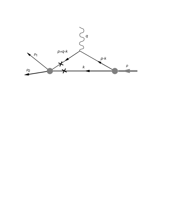
FIG. 8.: The two virtual particles in the final state can both be on shell (symbolized by the $\times$’s) if $W>m_{1}+m_{2}$.

To obtain a tractible form for the integral, replace the $u$ integration by $\beta$, which gives

$$T(Q^{2},W^{2})=\frac{1}{4\pi}\int^{1}_{0}dz\int^{(W^{2}-M^{2})z(1-z)}_{0}d\beta\;\;\frac{z(1-z)}{\sqrt{\gamma(z,\beta)}\,\left[\alpha_{W}(z)+\beta-i\epsilon\right]^{2}}\,,$$ (98)

where

$$\gamma(z,\beta)= {\textstyle{1\over 4}}[(W^{2}-M^{2})z(1-z)+Q^{2}z^{2}]^{2}-Q^{2}z^{2}\beta\,,$$ (99)

We now replace $W^{2}$ by

$$W^{2}=(p+q)^{2}=M^{2}+Q^{2}\left({1\over x}-1\right)\,$$ (100)

where $x$ is the Bjorken scaling variable

$$x={Q^{2}\over 2\,p\cdot q}={Q^{2}\over 2\,M\nu}\,,$$ (101)

and take the deep inelastic limit where $Q^{2}\to\infty$ with $x$ held constant. The integral is dominated by values of $z$ near zero, and hence may be approximated by

$$T(Q^{2},W^{2})\simeq \frac{x}{2\pi Q^{2}(1-x)}\int^{1}_{0}dz\int^{W^{2}z}_{0}d\beta\;\;\frac{1}{\left[m_{2}^{2}-W^{2}z+\beta-i\epsilon\right]^{2}}$$ (102)

$$\simeq \frac{x}{2\pi Q^{2}(1-x)}\int^{1}_{0}dz\left(\frac{1}{\left[m_{2}^{2}-W^{2}z-i\epsilon\right]}-\frac{1}{m_{2}^{2}}\right)$$ (103)

$$\simeq \frac{x}{2\pi Q^{2}(1-x)}\left({i\pi x\over Q^{2}(1-x)}-\frac{2}{m_{2}^{2}}\right)\,,$$ (104)

where we have kept the leading contribution from the imaginary part even though it is negligible compared to the real part.

In conclusion, one can state that the gauge invariant part of the rescattering term falls like $1/Q^{2}$. Noting that the bubble also falls as $1/Q^{2}$, the full rescattering term in the deep inelastic limit approaches

$${\cal J}^{\mu}_{b}\to-\left\{(p^{\prime}+p)^{\mu}-{q^{\mu}\,(p^{\prime 2}-p^{2})\over q^{2}}\right\}\;\frac{\lambda{\cal N}x}{\pi\,m_{2}^{2}\,Q^{2}(1-x)}\;$$ (105)

This is to be compared with the deep inelastic limit of the Born term, which is

$${\cal J}^{\mu}_{a}= -2\left(p_{1}^{\mu}-\frac{(q\cdot p_{1})}{q^{2}}q^{\mu}\right)\;\frac{{\cal N}}{m_{1}^{2}-(p_{1}-q)^{2}}\,,$$ (106)

and does not fall with $Q^{2}$. Hence, in the deep inelastic limit the gauge invariant part of the rescattering term is negligible in comparison to the gauge invariant part of the pole term.

In the next section we will calculate the cross section for deep inelastic scattering, and find the structure functions predicted by this simple model.

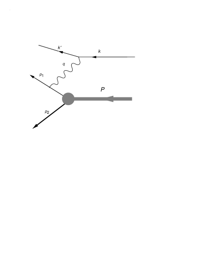
FIG. 9.: The leading contribution to DIS from a hadron.

V The nucleon structure functions

In this section we calculate the cross section and structure functions for the deep inelastic scattering (DIS) of unpolarized electrons from the composite “nucleon” $N$,

$$e+N\rightarrow e^{\prime}+X\,,$$ (107)

where $X$ is the undetected final hadronic state. This scattering process is illustrated in Fig. 9. The nucleon is composite, as described in Sec. II. For completeness, the well known kinematics and cross section formula[1, 2] are first reviewed in the next two subsections. The remaining subsections give results for the 1+1 D toy models presented in this paper.

A The Kinematics of DIS

The Bjorken variable, $x$, was defined in Eq. (101) and the invariant mass of the final hadronic state, $W$, in Eq. (100). In terms of these quantities, the energy transferred by the photon to the hadron in the lab system is

$$q^{0}=\nu=\frac{Q^{2}}{2Mx}$$ (108)

and the magnitude of the spatial component of $q$, which will be chosen to be in the $\hat{z}$ direction, is:

$$|{\bf q}|=q_{z}=\sqrt{Q^{2}+\frac{Q^{4}}{4M^{2}x^{2}}}\,.$$ (109)

In the CM of the outgoing hadronic pair, the invariant mass of the final state is

$$W=\sqrt{m_{1}^{2}+{\bf p}^{\prime 2}_{1}}+\sqrt{m_{2}^{2}+{\bf p}^{\prime 2}_{1}}\,,$$ (110)

where the prime denotes that the variable is evaluated in the CM system. The magnitude of the three-momentum of the “quark” (and “diquark”) in the CM frame, and in the Bjorken limit, is

$${\bf p}^{\prime 2}_{1}=\frac{\Delta(W^{2},m_{1}^{2},m_{2}^{2})}{4W^{2}}\rightarrow{Q^{2}(1-x)\over 4x}\left[1+{x(M^{2}-2m_{1}^{2}-2m_{2}^{2})\over Q^{2}(1-x)}\right]\,,$$ (111)

where the non-leading term will be needed below. The components of $q$ in the CM frame can be found by a Lorentz boost from the lab:

$$\pmatrix{q_{0}^{\prime}\cr 0\cr 0\cr q_{z}^{\prime}\cr}={1\over W}\pmatrix{\sqrt{W^{2}+{q}_{z}^{2}}&\;0\;&\;0\;&-q_{z}\cr 0&1&0&0\cr 0&0&1&0\cr-q_{z}&0&0&\sqrt{W^{2}+{q}_{z}^{2}}\cr}\pmatrix{q_{0}\cr 0\cr 0\cr q_{z}\cr}\,.$$ (112)

Hence the CM components are:

$$q_{0}^{\prime}= \frac{Q^{2}}{2Mx}\left[M^{2}+Q^{2}\left(\frac{1}{x}-1\right)\right]^{-1/2}\left[\left(M^{2}+\frac{Q^{2}}{x}+\frac{Q^{4}}{4M^{2}x^{2}}\right)^{1/2}-2Mx-\frac{Q^{2}}{2Mx}\right]$$ (113)

$$q_{z}^{\prime}= Q\left[M^{2}+Q^{2}\left(\frac{1}{x}-1\right)\right]^{-1/2}\sqrt{1+\frac{Q^{2}}{4M^{2}x^{2}}}$$ (115)

$$\qquad\times\left[\left(M^{2}+\frac{Q^{2}}{x}+\frac{Q^{4}}{4M^{2}x^{2}}\right)^{1/2}-\frac{Q^{2}}{2Mx}\right]\,.$$

In the deep inelastic limit these become

$$q_{0}^{\prime}= {Q(1-2x)\over 2\sqrt{x(1-x)}}\left[1-{M^{2}x\over 2Q^{2}(1-x)}\right]$$ (116)

$$q_{z}^{\prime}= {Q\over 2\sqrt{x(1-x)}}\left[1-{M^{2}x(1-2x)^{2}\over 2Q^{2}(1-x)}\right]\,,$$ (117)

where the non-leading terms will be needed later. Using the same boost, the energy of the initial hadron in the CM of the outgoing hadronic system is

$$p^{\prime}_{0}= \frac{M}{W}\sqrt{W^{2}+{q}^{2}_{z}}=\left[1+{Q^{2}\over M^{2}}\left(\frac{1}{x}-1\right)\right]^{-1/2}\left(M^{2}+\frac{Q^{2}}{x}+\frac{Q^{4}}{4M^{2}x^{2}}\right)^{1/2}$$ (118)

$$\to {Q\over 2\sqrt{x(1-x)}}\left[1-{M^{2}x[1-4(1-x)]\over 2Q^{2}(1-x)}\right]=q_{z}^{\prime}\left[1+{M^{2}\over 2q^{\prime 2}_{z}}\right]\,,$$ (119)

as expected. We now turn to the calculation of the cross section.

B Cross section and structure functions

The scattering amplitude for the DIS process is

$${\cal M}_{fi}={e^{2}\over Q^{2}}\,j_{e\,\mu}(k^{\prime},k){\cal J}^{\mu}_{a}\,,$$ (120)

where ${\cal J}^{\mu}_{a}$ is the hadronic current (kept general for now) and $j_{e\,\mu}(k^{\prime},k)$ is the current of the electron

$$j_{e\,\mu}(k^{\prime},k)=\overline{u}(k^{\prime}s^{\prime})\gamma_{\mu}u(k,s)\,.$$ (121)

The spins of the electron are denoted by $s$ and $s^{\prime}$, and the momenta are labeled as in Fig. 9. In this notation the unpolarized differential cross section in the lab is

$$\Delta\sigma= \int_{\Delta}\frac{d^{3}{k}^{\prime}\,d^{3}p_{1}\,d^{3}p_{2}\,}{(2\pi)^{9}32MEE^{\prime}E_{1}E_{2}}(2\pi)^{4}\delta(k^{\prime}+p_{1}+p_{2}-k-P)|{\cal M}_{fi}|^{2}$$ (122)

$$= {e^{4}\over Q^{4}}\,\int_{\Delta}\frac{d^{3}{k}^{\prime}}{(2\pi)^{3}8EE^{\prime}M}\;\ell^{\mu\nu}\,W_{\mu\nu}\,,$$ (123)

where $|{\cal M}_{fi}|^{2}$ contains a sum over the spins of the final particles and an average over the spins of the initial particles, $E_{1}$ and $E_{2}$ are the energies of the outgoing quark and diquark, $E$ and $E^{\prime}$ are the initial and final electron energies, and $\ell^{\mu\nu}$ and $W^{\mu\nu}$ are the lepton and hadron current tensors, defined below. The hadronic tensor contains all of the the physical information about the hadron-photon interaction and includes the integration over the outgoing hadrons and the normalization factors associated with the hadronic wave functions.

If the electron mass can be neglected the outgoing electron differential can be written $d^{3}k^{\prime}=E^{\prime 2}dE^{\prime}d\Omega^{\prime}$, which gives the following result for the inelastic cross section:

$$\frac{d^{2}\sigma}{d\Omega^{\prime}\,dE^{\prime}}=\frac{\alpha^{2}}{Q^{4}}\left(\frac{E^{\prime}}{E}\right){1\over 4\pi M}\,\ell^{\mu\nu}W_{\mu\nu}\,.$$ (124)

If the electron mass is neglected the lepton current tensor is

$$\ell_{\mu\nu}={1\over 2}\sum_{\rm spins}j^{\dagger}_{e\nu}j_{e\mu}=\frac{1}{2}Tr\left(\gamma_{\nu}\not k^{\prime}\gamma_{\mu}\not k\right)=2\left(k^{\prime}_{\mu}k_{\nu}+k_{\mu}k^{\prime}_{\nu}+\frac{1}{2}\,q^{2}g_{\mu\nu}\right)\,.$$ (125)

Gauge invariance of the hadronic current implies

$$q^{\mu}W_{\mu\nu}=W_{\mu\nu}q^{\nu}=0\,.$$ (126)

This in turn implies that the most general form of the hadronic tensor for unpolarized scattering is

$${W_{\mu\nu}\over 4\pi M}=-\left(g_{\mu\nu}-\frac{q_{\mu}q_{\nu}}{q^{2}}\right)W_{1}+\left(p_{\mu}-q_{\mu}\frac{p\cdot q}{q^{2}}\right)\left(p_{\nu}-q_{\nu}\frac{p\cdot q}{q^{2}}\right)\frac{W_{2}}{M^{2}}\,,$$ (127)

which defines the structure functions $W_{1}$ and $W_{2}$.

Substituting Eq. (127) into Eq. (124) gives

$$\frac{d^{2}\sigma}{d\Omega^{\prime}\,dE^{\prime}}= \left(\frac{2\alpha E^{\prime}}{Q^{2}}\right)^{2}\,\left[W_{2}\,\cos^{2}\left(\frac{\theta}{2}\right)+2W_{1}\,\sin^{2}\left(\frac{\theta}{2}\right)\right]$$ (128)

$$= \sigma_{M}\,\left[W_{2}+2W_{1}\,\tan^{2}\left(\frac{\theta}{2}\right)\right]\,,$$ (129)

where $\theta$ is the scattering angle of the electron in the lab system and $\sigma_{M}$ is the Mott cross section.

We now calculate the hadronic tensor. If the spin of the target is $S$, in 1+3 dimensions this tensor is

$$W_{\mu\nu}(q,p)= \frac{1}{(2S+1)}\sum_{S,s_{1},s_{2}}\int{d^{3}p_{1}^{\prime}d^{3}p_{2}^{\prime}\over(2\pi)^{6}4E^{\prime}_{1}E^{\prime}_{2}}(2\pi)^{4}\delta^{4}(p_{1}+p_{2}-q-p){\cal J}^{\dagger}_{a\nu}{\cal J}_{a\mu}$$ (130)

$$= \frac{1}{(2S+1)}\sum_{S,s_{1},s_{2}}\;{|{\bf p}^{\prime}_{1}|\over 4\pi(E^{\prime}_{1}+E^{\prime}_{2})}\,{1\over 4\pi}\,\int d\Omega^{\prime}_{1}\;{\cal J}^{\dagger}_{a\nu}{\cal J}_{a\mu}\,.$$ (131)

where $S$, $s_{1}$, $s_{2}$ are the spins, and the second line gives the result in the CM system. The volume integrals $d^{3}p_{1}/E_{1}$ and $d^{3}p_{2}/E_{2}$ are covariant, insuring that the tensor is also covariant. However, when we treat the hadronic degrees of freedom in 1+1 dimensions, consistency requires that the hadronic tensor also be evaluated in 1+1 dimensions. In this case Eq. (131) must be replaced by its 1+1 dimensional equivalent

$$W^{\prime}_{\mu\nu}(q,p)= \frac{1}{(2S+1)}\sum_{S,s_{1},s_{2}}\int{dp_{1}^{\prime}dp_{2}^{\prime}\over(2\pi)^{2}4E^{\prime}_{1}E^{\prime}_{2}}(2\pi)^{2}\delta^{2}(p_{1}+p_{2}-q-p){\cal J}^{\dagger}_{a\nu}{\cal J}_{a\mu}$$ (132)

$$= \frac{1}{(2S+1)}\sum_{S,s_{1},s_{2}}\frac{1}{4|{\bf p}^{\prime}_{1}|(E^{\prime}_{1}+E^{\prime}_{2})}\;\Bigl{\{}{\cal J}^{\dagger}_{a\nu}(+){\cal J}_{a\mu}(+)+{\cal J}^{\dagger}_{a\nu}(-){\cal J}_{a\mu}(-)\Bigr{\}}\,,$$ (133)

where the second line gives the result in the CM system with ${\cal J}_{a\mu}(\pm)$ corresponding to the cases when ${\bf p}^{\prime}_{1}$ is parallel to ${\bf q}$ (+) or antiparallel ($-$). Except for these two possibilities the delta functions completely fix the kinematics.

To calculate the structure functions for the 1+1 dimensional models, we use Eqs. (106), (58), and (LABEL:4eq7a). The definitions (LABEL:4eq7a) and (127) are covariant, so the structure functions can be evaluated in any frame, and it is convenient to evaluate them in the CM frame of the outgoing hadrons. Furthermore, since $q^{\prime}$ and $p^{\prime}$ have components only in the $\hat{t}$ and $\hat{z}$ directions, gauge invariance insures that

$$W^{0z}=W^{z0}={q^{\prime}_{0}\over q^{\prime}_{z}}W^{00}={q^{\prime}_{z}\over q^{\prime}_{0}}W^{zz}$$ (135)

and that $W^{yy}=W^{xx}$. Hence $W_{1}$ and $W_{2}$ can be extracted from

$$W^{xx}= 4\pi M\,W_{1}$$ (136)

$$W^{00}-W^{zz}= 4\pi M\,\left[\left(1+{Q^{2}\over 4M^{2}x^{2}}\right)W_{2}-W_{1}\right]\,.$$ (137)

In the next two subsections we calculate the structure functions for the scalar and spin 1/2 models in 1+1 dimensions.

C Structure functions for the scalar model

Using Eqs. (106) and (LABEL:4eq7a), the structure functions for the scalar theory in the deep inelastic limit are

$$W^{xx}= 0$$ (138)

$$W^{00}-W^{zz}= \frac{2x\;{\cal N}^{2}}{Q^{4}(1-x)}\;\left\{\frac{(q\cdot p_{1})^{2}}{(2q\cdot p_{1}-q^{2})^{2}}\,\Biggl{|}_{+}+\frac{(q\cdot p_{1})^{2}}{(2q\cdot p_{1}-q^{2})^{2}}\,\Biggl{|}_{-}\right\}\,,$$ (139)

where

$$(q\cdot p_{1})^{2}|_{+}= (q_{0}^{\prime}E_{1}^{\prime}-q^{\prime}_{z}p^{\prime}_{1})^{2}={\textstyle\frac{1}{4}}{Q^{4}}$$ (140)

$$(q\cdot p_{1})^{2}|_{-}= (q_{0}^{\prime}E_{1}^{\prime}+q^{\prime}_{z}p^{\prime}_{1})^{2}={\textstyle\frac{1}{4}}{Q^{4}}\;\left(\frac{1-x}{x}\right)^{2}$$ (141)

$$(2q\cdot p_{1}-q^{2})|_{+}= b-a$$ (142)

$$(2q\cdot p_{1}-q^{2})|_{-}= b+a\,,$$ (143)

and

$$a= 2{p}_{1}^{\prime}q^{\prime}_{z}\rightarrow{Q^{2}\over 2{x}}\left[1-{x\left(m_{1}^{2}+m_{2}^{2}-2M^{2}x(1-x)\right)\over Q^{2}(1-x)}\right]$$ (144)

$$b= Q^{2}+2E^{\prime}_{1}q^{\prime}_{0}\rightarrow Q^{2}+{Q^{2}(1-2x)\over 2{x}}\left[1-{x(m_{2}^{2}-m_{1}^{2})\over Q^{2}(1-x)}\right]$$ (145)

$$\rightarrow {Q^{2}\over 2{x}}\left[1-{x(1-2x)(m_{2}^{2}-m_{1}^{2})\over Q^{2}(1-x)}\right]\,.$$ (146)

Hence $b+a\to Q^{2}/x$, and the $(-)$ term vanishes in the deep inelastic limit. The (+) term is finite however, giving

$$W_{1}\rightarrow 0$$ (147)

$$\nu W_{2}\rightarrow {x\over 2\pi}(W^{00}-W^{zz})\rightarrow\frac{{x^{2}\;\cal N}^{2}}{4\pi(1-x)}\;\left(\frac{1}{b-a}\right)^{2}$$ (148)

$$\rightarrow \frac{{\cal N}^{2}}{4\pi}\;\frac{x^{2}\,(1-x)}{[m_{1}^{2}(1-x)+m_{2}^{2}x-M^{2}x(1-x)]^{2}}\,.$$ (149)

$W_{1}$ vanishes in the deep inelastic limit, as expected for scalar particles. But $\nu W_{2}$ scales in the deep inelastic region; its dependence on $Q^{2}$ and $\nu$ is replaced by dependence on the Bjorken scaling variable $x$ alone. In the simple quark parton model, we expect

$$\nu W_{2}(Q^{2},\nu)\rightarrow F_{2}(x)=xf(x)\,,$$ (150)

where $f(x)$ is the probability of finding a quark with momentum fraction $x$

$$\int_{0}^{1}dx\,f(x)=1\,.$$ (151)

Our simple model therefore predicts

$$f(x)=\frac{{\cal N}^{2}}{4\pi}\;\frac{x\,(1-x)}{[m_{1}^{2}(1-x)+m_{2}^{2}x-M^{2}x(1-x)]^{2}}\,,$$ (152)

which satisfies the normalization condition (151), as can be seen by comparing with Eq. (19).

D Structure functions for the spin 1/2 model

In the previous subsection we obtained the familiar result that the Callan-Gross relation[8] is not satisfied by scalar quarks. This relation predicts that

$$MW_{1}(Q^{2},\nu)\rightarrow F_{1}(x)={\textstyle\frac{1}{2}}f(x)\,,$$ (153)

where $f(x)$ the same function which specified $F_{2}$ in Eq. (150). For scalar quarks the structure function $W_{1}$ falls off with $Q^{2}$. To obtain the relation (153), the quarks must to be treated as spin 1/2 fermions. [The diquarks, even when their orbital angular momentum is zero, will have two spin states (0 and 1), and our choice of spin zero corresponds to the simplest possible wave function.] When carrying out the calculation in 1+1 D, we must assume that only the momenta are restricted to 1+1 D, but that the spin lives in the full 1+3 dimensional space. This assumption is fully consistent with the dynamical calculations of Secs. II and III.

From the spin zero calculation we know that it is sufficient to evaluate the (+) matrix element only. In this case the incoming nucleon is traveling in the $-\hat{z}$ direction, and the final quark in the $+\hat{z}$ direction. We will calculate this matrix element in the CM system of the outgoing pair using helicity states, which for this case are

$${U}_{N}(p,-\lambda_{N})= \sqrt{E_{p}+M}\pmatrix{1\cr-2\lambda_{N}{\tilde{p}}\cr}\chi_{{}_{\lambda_{N}}}$$ (154)

$$u(p_{1},\lambda_{1})= \sqrt{E_{p_{1}}+m_{1}}\pmatrix{1\cr 2\lambda_{1}{\tilde{p}}_{1}\cr}\chi_{{}_{\lambda_{1}}}$$ (155)

where

$${\tilde{p}}= \frac{p}{E_{p}+M}\simeq 1-\frac{M}{p}$$ (156)

$${\tilde{p}}_{1}= \frac{p_{1}}{E_{p_{1}}+m_{1}}\simeq 1-\frac{m_{1}}{p_{1}}$$ (157)

$$\chi_{+}= \pmatrix{1\cr 0\cr}\qquad\chi_{-}=\pmatrix{0\cr 1\cr}\,.$$ (158)

With the help of these quantities, the $x$-component of the current (58) becomes:

$${\cal J}_{a}^{x}= \sqrt{(E_{p_{1}}+m_{1})(E_{p}+M)}\,\frac{{\cal N}}{b-a}\;2\lambda_{N}\,[q^{0}({\tilde{p}}_{1}-{\tilde{p}})+q^{3}({\tilde{p}}_{1}{\tilde{p}}-1)]\,\delta_{\lambda_{N},\lambda_{1}}$$ (159)

$$\rightarrow -\frac{{\cal N}Q}{\sqrt{x}\,[b-a]}\;2\lambda_{N}\,[Mx+m_{1}]\,.$$ (160)

This gives

$$W_{1}={{\cal N}^{2}\over 8\pi M}\;\frac{(1-x)(Mx+m_{1})^{2}}{[m_{1}^{2}(1-x)+m_{2}^{2}x-M^{2}x(1-x)]^{2}}={\frac{1}{2M}}f(x)$$ (161)

In a similar manner, it may be shown that $W^{00}-W^{zz}\to 0$ in the deep inelastic limit, which is the Callan Gross relation [recall Eq. (137)].

Note that the normalization condition for the spin 1/2 model given in Eq. (31) confirms that this model is also correctly normalized. However, the $f(x)$ obtained from the spin 1/2 model does not go to zero as $x\to 0$.

E Numerical results

In Fig. 10 the structure functions obtained from the scalar and spin 1/2 models are compared with the empirical momentum distribution $xu(x)$ for $u$ quarks in the proton. The empirical distribution was taken from Ref. [9] and has been renormalized to unity for comparison.

Note that the parameters in the momentum distributions predicted by the models can be chosen to give a qualitatively reasonable description of empirical results, but the models fail at both large and small $x$. The large $x$ distributions fall like $1-x$, while the empirical distribution falls more rapidly (the fit gives $(1-x)^{3.509}$ compared to $(1-x)^{3}$ for the naive quark model). Similarly, the empirical distribution goes like $x^{0.4810}$ at small $x$, while the spin 1/2 model goes like $x$ and the scalar model goes like $x^{2}$. Assuming the $u$ and $d$ quark distributions are identical, the resulting momentum carried by valence quarks is $3\times 0.150=0.450$ for the empirical distribution, $3\times 0.210=0.630$ for the spin 1/2 model, and $3\times 0.232=0.696$ for the scalar model. In every case some momentum must be carried by glue or sea quarks, and the naive models presented here do not include these contributions. This will be investigated in a future work.

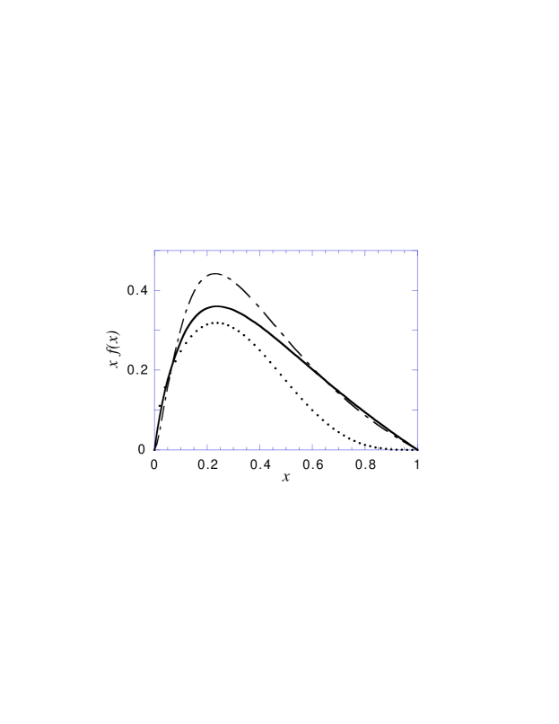
FIG. 10.: Quark momentum distributions: $xu(x)$ with $u(x)$ normalized to unity (dotted line), $xf(x)$ for the scalar model with $m_{1}^{2}/M^{2}=0.1$ and $m_{2}^{2}/M^{2}=2$ (dashed line), and $xf(x)$ for the spin 1/2 model with $m_{1}^{2}/M^{2}=0.18$ and $m_{2}^{2}/M^{2}=2$ (solid line).

VI CONCLUSIONS

In this paper we have shown how to extract the gauge invariant part of the pole term so that it gives the leading contribution to deep inelastic scattering. The gauge non-invariant part depends only on $q^{\mu}$ and is cancelled exactly by the rescattering term. While we have not shown it explicitly, the argument suggests that this procedure is quite general and works as follows. First add a (unique) term proportional to $q^{\mu}$ to the pole term which makes it gauge invariant. Then subtract the same term from all of the remaining terms (rescattering and interaction currents). It follows that the remaining terms are also gauge invariant, and we conjecture that the sum of all of these remaining terms will vanish in the deep inelastic limit. Hence the modified pole term will give the exact result for DIS.

More explicitly, imagine that the full current is the sum of a pole term $J_{\rm pole}^{\mu}$ and a remainder $J_{\rm rem}^{\mu}$, and that it is gauge invariant. The first step is to write it as

$$J^{\mu}= J_{\rm pole}^{\mu}+J_{\rm rem}^{\mu}$$ (162)

$$= \left(J_{\rm pole}^{\mu}-\alpha\,q^{\mu}\right)+\left(J_{\rm rem}^{\mu}+\alpha\,q^{\mu}\right)\,,$$ (163)

where

$$\alpha=\frac{J_{\rm pole}\cdot q}{q^{2}}\,.$$

Note that $\alpha$ is uniquely determined (unless $q^{2}=0$, which cannot happen for DIS), and that the modified pole term

$$J_{\rm modpole}^{\mu}=J_{\rm pole}^{\mu}-\frac{J_{\rm pole}\cdot q}{q^{2}}\;q^{\mu}$$ (164)

is gauge invariant by construction. We conjecture that the modified remainder terms (which are also gauge invariant) will vanish in the DIS limit, leaving (164) to give the exact result for DIS. Note that our prescription (164) is identical to the Landau prescription, and defined in Ref. [5].

The second result of this paper is the construction of toy models for the discription of DIS. These models give a qualitatively reasonable description of the phenomenology, as shown in Fig. 10, but simplicity is their main virtue. We plan to use them to study many issues in the theory of DIS.

- [1] G. W. West, Phys. Rep. 18, 263 (1975).
- [2] R. G. Roberts, The Structure of the Proton (1990).
- [3] F. Gross and S. Liuti, Phys. Rev. C 45, 1374 (1992); A. Yu. Umnikov and F. C. Khanna, Phys. Rev. C 49, 2311 (1994); W. Melnitchouk, A. W. Schreiber, and A. W. Thomas, Phys. Lett. B335, 11 (1994); W. Melnitchouk, G. Piller, and A. W. Thomas, Phys. Lett. B346, 165 (1995).
- [4] T. de Forest, Jr. Nucl. Phys. A392, 232 (1983); Ann. Phys. (N.Y.) 45, 365 (1967).
- [5] J. Kelly, Phys. Rev. C 56, 2672 (1997).
- [6] M. Einhorn, Phys. Rev. D 14, 3451 (1976).
- [7] F. Gross and D. O. Riska, Phys. Rev. C 36, 1928 (1987).
- [8] C. Callan and D. Gross, Phys. Rev. Lett. 22, 156 (1969).
- [9] J. C. Collins and Wu-Ki Tung, Nucl. Phys. B278, 934 (1986). These fits were provided to us by C. Wahlquist.