MKPH-T-97-34

1 Introduction

The goal of the group was to summarize the current status of our knowledge on form factors and polarizabilities of hadrons, and to identify experimental and theoretical activities which could give new and significant information. These were 4 days of stimulating talks and discussions. The agenda was a mixture of experiment and theory with the aim to have frank and critical discussions on the current issues. The topics covered by the working group are presented as follows.

The status of hadron form factors is reviewed in Section 2. Experimental data for the nucleon were presented for both time-like and space-like momentum transfers by E. Luppi and F. Klein. These two experimentally disjunct regions are connected by dispersion relations as discussed by G. Höhler, A. Z. Dubničkov$\acute{\mbox{a}}$ and S. Dubnička. U.-G. Meißner presented new calculations of the spectral functions in the framework of ChPT, and H.-W. Hammer reported on a dispersion calculation for the strangeness vector current. The relevance of double polarization for improving on the neutron data basis was stressed by J. Becker and M. Ostrick. Finally, T. Hannah reported on calculations of the pion form factor by the inverse amplitude method.

Section 3 is devoted to the polarizability of hadrons as seen by Compton scattering. V. Olmos described a Mainz experiment supposed to yield new precision values for the (scalar) polarizabilities of the proton, and D. Hornidge showed new data for Compton scattering off the deuteron. The current status of ChPT calculations of the spin (or vector) polarizabilities was reviewed by Th. Hemmert. Finally, L. Fil’kov described a Mainz experiment to measure the pion polarizability by radiative pion photoproduction, and A. L’vov reported on a proposal to study the Compton amplitude by lepton pair production.

Section 4 covers the field of virtual Compton scattering (VCS), which has the potential to give information on the spatial distribution of the polarizabilities. S. Scherer gave an introduction to a VCS calculation in the framework of ChPT, and A. Metz reported on relations between the generalized polarizabilities (GPs) measured by VCS. A designed experiment to measure the GPs at MIT/Bates was presented by R. Miskimen, and J. Roche described the preliminary results of such measurements at MAMI.

2 Hadron Form Factors

The form factors of hadrons have been studied by electron scattering and pair annihilation or creation. The virtual photon exchanged in these reactions has four-momentum q, and $t=q^{2}$ defines the Mandelstam variable. In the case of pair annihilation the momentum transfer is time-like, $q^{2}\geq 4m^{2}_{N}$, electron scattering probes the form factors at space-like momentum transfer, $q^{2}<0$. Fig. 1 shows the existing data and a model-calculation for the magnetic form factor of the proton for both time- and space-like momentum transfers [1]. The form factor is real for $t<4m_{\pi}^{2}$ or $9m_{\pi}^{2}$ for its isovector or isoscalar part, respectively, it becomes complex above these lowest thresholds corresponding to two- or three-pion production. The spikes in the unphysical region $0\leq t\leq 4m_{N}^{2}$ correspond to vector mesons, which dominate the imaginary part of the form factor.

Figure 1: The magnetic form factor of the proton $\mid G_{M}^{p}\mid$ as function of $t$. See text.

The status of the nucleon form factors in the time-like region was reviewed by E. Luppi. Data were presented from both the reaction $N\bar{N}\rightarrow e^{+}e^{-}$ (E760, PS170) [2, 3] and the inverse reaction (FENICE)[4]. The differential cross section for this process defines the electric $(G^{N}_{E})$ and magnetic $(G^{N}_{M})$ Sachs form factors of the nucleon [5],

$$\frac{d\sigma}{d\Omega}=\frac{\alpha^{2}\beta_{N}}{4t}\left(|G^{N}_{M}(t)|^{2}(1+\cos^{2}\theta)+\frac{4m^{2}_{N}}{t}|G^{N}_{E}(t)|^{2}\sin^{2}\theta\right),$$ (1)

with $\beta_{N}$ the velocity of the nucleon and $\theta$ the production angle. Up to now the angular distributions have been measured only with large error bars, particularly in the case of the neutron. Taken at face value, the form factors of proton (p) and neutron (n) are related by the data as follows:

$$|G^{p}_{E}|\approx|G^{p}_{M}|,\ \ |G^{p}_{M}|<|G^{n}_{M}|,\ \ |G^{n}_{M}|\gg|G^{n}_{E}|.$$ (2)

Since the electric and magnetic Sachs form factors at threshold are equal by definition,

$$G^{N}_{E}(4m^{2}_{N})=G^{N}_{M}(4m^{2}_{N}),$$ (3)

the relations eq.(2) would require a resonating behaviour of $G^{n}_{M}$ very close to threshold. In general the magnetic form factors are better known, because the electric ones are suppressed by kinematical factors in in most experiments. The experimental results for the proton form factor in the time-like region are presented in Fig. 2. In particular they include the experiments $PS170$ at CERN [3] in the range between threshold and $q^{2}=4.2GeV$, and $E760$ at Fermilab [2] in the region $8.9\leq q^{2}/GeV^{2}\leq 13$. The FENICE results are obtained by $e^{+}e^{-}$pair annihilation, and evaluated under the hypothesis $\mid G_{E}^{p}\mid=\mid G_{M}^{p}\mid$. Though the threshold data have still large error bars, the indication of a “resonance” in the form factors near threshold is quite strong. This may be related to a dip in the total cross section for $e^{+}e^{-}\rightarrow$ hadrons at about 1.87 GeV with a small width of about 10 MeV. Another point of interest is the predicted asymptotic scaling of the form factor, i.e. $q^{4}|G|\rightarrow$ const for large values of $q^{2}$. As may be seen in Fig. 2 this quantity is rather constant in the region $q^{2}>8GeV^{2}$. However, it stays at about twice the level reached at the corresponding momentum transfer in the space-like region (i.e. for $q^{2}<-8GeV^{2}$)! This is a clear indication that asymptotia is not yet reached in the region of $10-20GeV^{2}$.

Figure 2: The magnetic form factor of the proton $\mid G^{p}\mid q^{4}/\mu_{p}$ as function of $s=q^{2}$ in the time-like region.See text.

The form factor of the neutron is shown in Fig. 3. The result at $\sqrt{s}=1.9GeV$ is shown as a shaded area corresponding to two different hypotheses for the $c.m.$ energy of the accelerator. The neutron form factor is considerably larger than the proton one over the whole energy range and, surprisingly, the magnetic neutron form factor is found to be much larger than the electric one.

Clearly, the unexpected results in the time-like region deserve future attention. Therefore, the Fenice Group is studying possibilities to improve the data by a high luminosity, asymmetric $e^{+}e{-}$ collider with a high energy $e^{+}$ storage ring and a high intensity $e^{-}$ linac.

Figure 3: The magnetic form factor of the neutron $\mid G_{M}^{n}\mid$ as function of $q^{2}$ in the time-like region. See text.

F. Klein reported on the status of the space-like nucleon form factor. The differential cross section in this region is given by

$$\frac{d\sigma}{d\Omega}=\sigma_{p}\left(\frac{G^{2}_{E}+\tau G^{2}_{M}}{1+\tau}+2\tau G^{2}_{M}\tan^{2}\frac{\theta}{2}\right),$$ (4)

with $\tau=Q^{2}/4m^{2}_{N}$, $Q^{2}=-q^{2}$, and $\theta$ the scattering angle. Except for the electric form factor of the neutron, the form factors follow the dipole shape, $G^{p}_{E}\approx G^{p}_{M}/\mu_{p}\approx G^{n}_{M}/\mu_{n}\approx(1+Q^{2}/0.71GeV^{2})^{-2}$. From a nonrelativistic, and somewhat questionable point of view, this form factor corresponds to an exponential charge distribution as function of the radius r, $\rho(r)=\rho_{0}exp(-r/r_{0})$.

Due to the kinematical factors in eq. (4), $G^{p}_{E}$ dominates at small values of $Q^{2}$ and $G^{p}_{M}$ at large ones. This makes it difficult at both small and large $q^{2}$, to separate the two form factors by studying the angular dependence at $Q^{2}=const$ (“Rosenbluth plot”). For the proton precise electron scattering data are available from single arm experiments up to momentum transfers $Q^{2}=30GeV^{2}/c^{2}$. A Rosenbluth separation was made [6, 7] up to $9GeV^{2}/c^{2}$ while for higher $Q^{2}\;,\;G_{M}$ was directly taken from the cross section with the small $G^{p}_{E}$-contribution $(\leq 5\%)$ subtracted. This limit may be pushed upwards in $Q^{2}$ in double polarization experiments which are planned or in preparation. In particular, the data at lower $Q^{2}$ can be substantially improved by means of double polarization experiments at the new electron accelerators in the GeV region. It is worth pointing out that even a new measurement of the electric $rms$ radius of the proton may be interesting. This quantity was determined by a series of Mainz experiments in the 70’s as $r^{p}_{E}=(0.862\pm 0.012)fm$ [8]. It tends to be somewhat smaller in a global fit to the data performed in the framework of dispersion theory, $r^{p}_{E}=(0.847\pm 0.008)fm$ [9]. However, these small uncertainties are now the limiting factor in atomic physics investigations to check the validity of QED [10]!

For obvious reasons the situation is worse in the case of the neutron. Precise numbers exist only for its electric radius as determined by the transmission of low energy neutrons through Pb atoms [11],

$$\left<r^{2}\right>^{n}_{E}=(-0.113\pm 0.003\pm 0.004)fm^{2},$$ (5)

indicating a small value for the Dirac form factor $F_{1}^{n}$. On the contrary, at high momentum transfers the observed smallness of $G_{E}^{n}$ [12] demands a finite value for $F_{1}^{n}$. The older neutron data rely mostly on quasi free scattering off the neutron bound in ${}^{2}H$. In that approximation the longitudinal and transverse structure functions determine $\left(G^{n}_{E}\right)^{2}$ and $\left(G^{n}_{M}\right)^{2}$, respectively. Since $G^{n}_{E}(0)=0$ and $G^{n}_{E}\ll G^{p}_{E}$ at all the measured $Q^{2}$ values, the electric neutron form factor obtained by this method is essentially zero with a large error bar. Concerning $G^{n}_{M}$, the SLAC data [6] cover the region between $1.5GeV^{2}$ and $4GeV^{2}$ with relatively small error bars. At the smaller momentum transfer the data scatter considerably. Though there exist more recent data from NIKHEF [13], Mainz [14] (preliminary) and Bonn [15] with small error bars, the Bonn data are systematically higher by about $10\%$. It is obvious that this discrepancy requires further investigations.

Relatively precise values for $G^{n}_{E}$ were obtained by elastic scattering off the deuteron under the assumption that the contributions of the proton, the internal wave function and two-body currents are well under control [16]. In order to obtain more model-independent results, double polarization experiments have been proposed with the aim to measure asymmetries, e.g.

$${}^{3}\vec{H}e(\vec{e},e^{\prime}n),\ \ D(\vec{e},e^{\prime}\vec{n})\quad\mbox{and}\quad\vec{D}(\vec{e},e^{\prime}n).$$ (6)

The first of these reactions has been studied at Mainz and the results were presented by J. Becker, the second one has been scheduled at MIT/Bates and measured at Mainz (preliminary results presented by M. Ostrick), and the third one is being pursued at Jefferson Lab.

As pointed out by Ref. [17], the asymmetry in a double polarization experiment takes the form

$$A=P_{e}P_{n}\frac{aG^{n}_{E}G^{n}_{M}\sin\Theta+b(G^{n}_{M})^{2}\cos\Theta}{c(G^{n}_{E})^{2}+d(G^{n}_{M})^{2}},$$ (7)

where $P_{e}$ and $P_{n}$ are the polarization of the incoming electron and the target or recoiling neutron, respectively, and a, b, c, d are known kinematical functions. The angle $\Theta$ is the angle between the momentum $\vec{q}$ of the virtual photon and the neutron spin in the scattering plane of the electron, i.e. $\Theta=0$ if the neutron spin points in the direction of $\vec{q}$, and $\Theta=90^{\circ}$ if perpendicular to $\vec{q}$, in the scattering plane and to the same side as the momentum of the outgoing electron. In the latter kinematics the asymmetry $A_{\perp}$ essentially measures $G^{n}_{E}/G^{n}_{M}$, while the parallel asymmetry $A_{\parallel}$ is practically independent of the form factors because of the small value of $G^{n}_{E}$. Particularly in the case of the deuteron target, there are convincing arguments that the analysis of these double polarization experiments is only little affected by two-body currents and binding effects [18]. In this sense the new data for $G^{n}_{E}$ should be rather model-independent.

Concerning the reaction $D(\vec{e},e^{\prime}\vec{n})$ at MAMI [19], the scattered electrons were detected in an array of lead glass detectors. The energy information $(\Delta E/E\approx 20\%)$ was used to suppress non quasifree events. The neutron were detected in coincidence in a wall of plastic scintillators. The detection process itself provides the analyzing power for the extraction of polarization components transverse to the direction of neutron momentum. An experimental calibration of the polarimeter at a polarized neutron beam can be circumvented by using the spin precession in a magnetic field. On their way through a magnet with a field perpendicular to the scattering plane, the neutrons undergo a spin precession. The angle $\Theta_{0}$ of zero crossing of the asymmetry $A$ of eq. (7) is directly related to the ratio of the electric and magnetic form factors,

$$\tan\Theta_{0}=-\frac{a}{b}\cdot\frac{G_{E}}{G_{M}},$$ (8)

and depends neither on the absolute values of the polarimeter’s analyzing power nor on the electron beam polarization. Kinematical cuts change the amplitude, i.e. the effective analyzing power, but not the zero crossing angle $\Theta_{0}$.

The reaction ${}^{3}\vec{He}(\vec{e},e^{\prime}n)$ was measured at MAMI in the range of momentum transfer Q²=0.27-0.5 GeV². ${}^{3}\vec{He}$ serves as an effective polarized neutron target with its spin oriented in perpendicular or parallel direction to the momentum transfer. The experiment quantifies the respective asymmetries whose ratio $A_{\perp}/A_{\|}$ is independent of the polarization degrees of electron beam and target and of a dilution of the two asymmetries due to unpolarized background. The PWIA analysis is based on an event–by–event kinematical reconstruction that is supported by a Monte Carlo simulation. The analysis considers the kinematical acceptance of the detector system ($\Delta\Omega_{e}$=100 msr) and provides an efficient selection of quasi–elastic scattering with low missing momentum ($|\vec{P}_{m}|$$\leq$100 MeV/c). The final step of this analysis is a Monte Carlo adaptation of the reconstructed kinematics which takes account of the effects that can not be determined for the single event but are known from their statistical distributions: missing energy, radiation losses and energy losses of the neutrons in the lead shielding of the neutron detector. Test measurements with H₂– and D₂–filled target cells examined the contribution to the signal due to (p,n)–charge conversion in this lead shielding which could be reduced to a fraction of 4% in the event–by–event reconstruction. With a value of 1.05$\pm$0.05 times the dipole fit for G${}_{M}^{n}$ the Q²–averaged result is G${}_{E}^{n}$=0.0352$\pm$0.0033$\pm$0.0024 [20]. This result is shown in Fig. 4 together with an earlier exploratory ³He–experiment [21], the preliminary results of the deuteron experiments [19] and data extracted from elastic electron scattering off deuterium [16]. The four lines in the plot are two-parameter fits to the data set of [16] by use of different nucleon-nucleon potentials in the calculation of the deuterium wave function. Data points are plotted for the case of the analysis with the Paris potential (fit: solid line). The ³He experiment will be continued at higher momentum transfer, $Q^{2}$=0.67 GeV², at the MAMI spectrometer facility (A1–collaboration) [22].

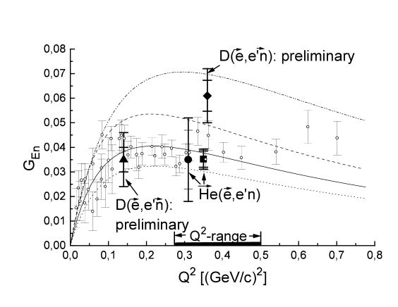
Figure 4: The electric form factor of the neutron $G_{E}^{n}$ as function of $Q^{2}$. Full circles: exploratory ³He experiment [21]; full squares: full ³He experiment (stat. and quadr. added total error) [20]; full triangle and full diamonds: D experiment [19], preliminary; lines and open points: elastic $D(e,e^{\prime})$ [16], see text.

As may be seen in Fig. 4, the preliminary results for the deuteron are higher than for the ${}^{3}He$ experiment. There are three possible explanations for this effect, systematical errors in one or the other experiment, problems with final state interactions and two-body currents in ${}^{3}He$ (a complete Faddeev calculation for the reaction is still missing), and possible modifications of the nucleon’s form factors in the medium. Of course, the latter possibility would be a most interesting effect which has been under discussion and looked for in many investigations. With regard to such medium effects one has to keep in mind that the factor 2 between the two experimental values at $Q^{2}\approx.35GeV^{2}$ could be achieved by shifting only a relatively small amount of charge in the neutron, because the positive core and the negative cloud are of equal size and small. A similar change of the form factor of the proton by an absolute value of about 0.03 would be much less exciting. In conclusion it is obvious that $G^{n}_{E}$ is particularly sensitive to the details of models describing the hadronic structure. Therefore, further activities to measure this quantity with better accuracy and improved data analysis should be strongly encouraged.

The most quantitative description of the electromagnetic form factors can be obtained within the framework of dispersion theory for the Dirac and Pauli form factors $F_{1}$ and $F_{2}$, e.g.

$$F_{2}(t)={1\over\pi}\,\int_{t_{0}}^{\infty}\,{{\rm Im}~{}F_{2}(t^{\prime})\over t^{\prime}-t-i\varepsilon}\,\,,$$ (9)

where the spectral function (SF) ${\rm Im}~{}F(t)$ encodes the pertinent physics. It is well known that the isovector SF has a significant enhancement on the left wing of the $\rho$ meson due to a singularity on the second Riemann sheet at $t_{c}=4m_{\pi}^{2}-m_{\pi}^{4}/m_{N}^{2}$ close to the threshold $t_{0}=4m_{\pi}^{2}$ (for a detailed discussion, see [23]). This is also found in chiral perturbation theory (CHPT) at one loop as first observed in [24]. One can therefore ask the question whether a similar phenomenon appears in the isoscalar channel, i.e. on the left wing of the $\omega$ meson. For that, one has to analyze the two–loop diagrams depicted in Fig. 5 [25]. Although the solution of the pertinent Landau equations reveals a singularity on the second sheet at $t_{c}=8.9m_{\pi}^{2}$, i.e. close to the physical isoscalar threshold at $t_{0}=9m_{\pi}^{2}$, there is no enhancement as shown in Fig. 5 (right panel) due to the three–body phase space factors. The nonresonant part of the SF related to the three–pion continuum is very small and rises smoothly with increasing $t$. Consequently, it is justified to saturate the isoscalar SF at low $t$ by the $\omega$. The same is found for the SF of the nucleon isovector axial from factor [25].

Figure 5: Right: Isoscalar spectral functions weigthed with $1/t^{2}$ for the electric (lower curve) and magnetic (upper curve) Sachs form factors. Left: the underlying two–loop graphs (solid, dashed, wiggly lines: nucleons, pions and photons). Calculations by Bernard, Kaiser and Meißner [25].

The first peak of the spectral function of the isoscalar vector form factor is due to $\omega$ exchange. Its height is proportional to the coupling constant $g_{1}(\omega NN)$. One would expect that the values of this coupling constant found in analyses of different groups get closer with the recent improvements of the experimental data base. Unfortunately, this is not true. The values show large fluctuations even in recent years.

The main reason was pointed out in [26]: the calculation of the spectral function from the data is a mathematically ill-posed problem. If a fit with a “good” $\chi^{2}$ has been found, there exists a large number of other solutions with the same $\chi^{2}$ but quite different spectral functions which usually show additional oscillations. In Ref. [26] a stable analytic continuation was applied which was justified in Ref. [27]. The number of adjustable parameters was reduced by calculating the $\rho$ contribution from a continuation of $\pi N$ amplitudes and p-wave $\pi\pi$ phase shifts.

In a recent paper [9] this method was improved and new data were taken into account. The authors obtained $g_{1}^{2}(\omega NN)/4\pi=34.6\pm 0.8$, close to the old value. Other recent results vary in the range from 4 to 363. Some of the reasons for this were pointed out in Ref. [28], and one should keep in mind that structures of spectral functions are not necessarily due to vector mesons and that the experimental information on higher $\rho$ and $\omega$ states is rather poor.

Concerning the values of coupling constants determined from nucleon-nucleon scattering, $g_{1}^{2}(\omega NN)/4\pi=8.1\pm 1.5$ was found in a careful study of the dispersion relations for $NN$ forward scattering [29]. The $\phi$ contribution was assumed to be zero. Otherwise the $\omega$ coupling would become smaller. Results from OBE models of the NN force have the problem that, in contrast to couplings in dispersion theory, the $\omega$ is off-shell, at $t\approx 0$ rather than at $t=m^{2}_{V}$. The extrapolation to the on-shell value is very model-dependent, leading to typical values of $g^{2}_{1}/4\pi=20$ [30]. Obviously the large coupling constant found by form factor analyses would require a larger $\omega NN$ transition radius than used in OBE models.

The slope of the Dirac isoscalar form factor at $t=0$ can be obtained rather accurately from the slope of the electric Sachs form factor of the proton and the form factor of the neutron, $F^{\prime}_{1s}(0)=1.36\,GeV^{-2}$. The first two terms of the result of Mergell et al. [9] due to the $\omega$ and the $\phi$ terms are $F^{\prime}_{1s}(0)=(2.00-0.683)=1.32\,GeV^{-2}$. If we use the coupling constant of Grein et al., the $\omega$ contribution is only 1.00 and therefore smaller than the experimental value. It is then not possible to describe that $F_{1s}(t)$ behaves approximately like the usual dipole fit.

A. Z. Dubničkov$\acute{\mbox{a}}$ explained that the large $\omega$ coupling comes about if the dipole form is constructed by $\omega$ and $\phi$ poles, while a much smaller coupling is needed if the dipole is made up of $\omega$(782) and $\omega^{\prime}$ (1420). Under the usual conditions of normalization and asymptotic behaviour of the form factor, she obtained $g^{2}_{1}(\omega NN)/4\pi\approx 34$ for $\omega$ and $\phi$ poles, and $g^{2}_{1}(\omega NN)/4\pi\approx 12$ for $\omega$ and $\omega^{\prime}$ poles. Of course the latter assumption requires to introduce a strong coupling to the $\omega^{\prime}$.

S. Dubnička presented a model of the form factors based on the resonances $\omega$(782), $\phi$(1020), $\omega^{\prime}$(1420), $\omega^{\prime\prime}$(1600), $\phi^{\prime}$(1680) and $\rho$(770), $\rho^{\prime}$(1450), $\rho^{\prime\prime}$(1700), $\rho^{\prime\prime\prime}$(2150), and $\rho^{\prime\prime\prime\prime}$ (2600). All these resonances are experimentally confirmed, except for the $\rho^{\prime\prime\prime}$(2150), taken from [31] and the $\rho^{\prime\prime\prime\prime}$(2600) which has been postulated to reproduce the time-like data of the E760 experiment [2]. The large number of free parameters is somewhat reduced by requiring the usual normalization and asymptotic conditions. Applying special nonlinear transformations [32] and incorporating the finite widths of the vector mesons, the model describes all existing data in both the space-like and the time-like region.

In the discussion there was some criticism with regard to the large number of vector mesons introduced in this model, which produces large and possibly unphysical oscillations. Except for the possible resonance at 1.87 GeV, the higher resonances are not (yet) shown by the data. However, a closer look for such resonances in the time-like region by more precise experiments will be worthwhile the effort.

The contribution of strange quarks to the nucleons’s structure has been another topic of interest. Experiments to measure the strange form factors of the nucleon by parity-violating electron scattering are being pursued at MIT/Bates, Jefferson Lab and MAMI, and first results on the strangeness contribution of the magnetic moment were obtained at MIT/Bates [33]. The theoretical investigations of this effect were based on dispersion relations, kaon-loop calculations and Skyrme models, and resulted in various predictions differing both in sign and in magnitude. H.-W. Hammer reported on recent studies of the strange vector form factors of the nucleon in the framework of dispersion relations (DR) [34],

$$\bar{u}(p)\left[Im\,F^{s}_{1}(t)\gamma_{\mu}+i\frac{Im\,F^{s}_{2}(t)}{2m_{N}}\sigma_{\mu\nu}(\bar{p}+p)^{\nu}\right]v(\bar{p})$$ (10)

$$\qquad\qquad\qquad\qquad\qquad\sim\sum_{n}\langle N(p)\bar{N}(\bar{p})\mid n\rangle\langle n\mid\bar{s}\gamma_{\mu}s\mid 0\rangle\,\delta^{4}(p+\bar{p}-p_{n}).$$

The sum over the intermediate states was saturated by $K\bar{K}$ and $3\pi$ intermediate states, which are the lightest (isoscalar) states containing strange and nonstrange particles, respectively. Due to the $1/t$ or $1/t^{2}$ weighting factors these states are the most important ones in the DR. In most previous model calculations only contributions of the kaon cloud have been included (kaon cloud dominance), because the OZI-rule would not allow for matrix elements such as $\langle 3\pi\mid\bar{s}\gamma_{\mu}s\mid 0\rangle$.

For the $K\bar{K}$ continuum, the effects of unitarity, a realistic kaon strangeness form factor, and the inclusion of $KN$ scattering data were studied and compared to a model calculation in the nonlinear $\sigma$-model [35, 36]. The dispersion integral splits into the physical region ($t\geq 4m^{2}_{N}$) with experimental data for the scattering amplitude $\langle N\bar{N}\mid K\bar{K}\rangle$ and the unphysical region ($4m^{2}_{K}\leq t\leq 4m^{2}_{N}$) for which an analytical continuation is needed. The constraints from unitarity of the $S$-matrix for the $K\bar{K}\rightarrow N\bar{N}$ amplidudes reduce the contribution from the physical region by a significant amount. As a consequence, the main contribution of the dispersion integral is from the unphysical region where unitarity does not apply. As an example,the nonlinear $\sigma$-model violates the unitarity bounds by a factor of 3 or more. Moreover, the impact of realistic parametrizations for the matrix element $\langle K\bar{K}\mid\bar{s}\gamma_{\mu}s\mid 0\rangle$, i.e. the kaon strangeness form factor $F^{s}_{K}$, is significant. Comparison with the corresponding electromagnetic quantity indicates a strong effect of the $\phi(1020)$ enhancing the $K\bar{K}$ threshold region in the dispersion integral. Furthermore, the experimental $K^{+}N$-scattering amplitudes have been analytically continued to the $t$-channel unphysical region by means of backward DR [36]. This technique provides the two $t$-channel $J=1$ partial waves that determine the spectral functions together with the kaon strangeness form factor $F^{s}_{K}$. The analytical continuation results in a resonance structure near $K\bar{K}$ threshold, presumably due to the $\phi(1020)$. In combination with $F^{s}_{K}$ this increases the $K\bar{K}$ contribution to the electric radius to $\rho^{s}_{E}=-(2m^{2}_{N}/3)\left<r^{2}\right>^{s}_{E}\approx 1$, which is at a level observable in the proposed experiments. Obviously the one-loop model calculations yield only a highly incomplete picture of the underlying physics, because they neglect the resonance effects in both kaon strangeness form factor and $K\bar{K}\rightarrow N\bar{N}$ partial waves and the rescattering effects in the latter. The predicted increase in the strangeness radius reduces the discrepancy between vector meson pole and $K\bar{K}$ continuum results, indicating a possible solution for this longstanding problem.

The $3\pi$ continuum is the lowest mass intermediate state in the spectral decomposition of Eq. (10). Therefore its contribution is substantially enhanced in the DR in comparison with the kaon cloud. Since the nonresonant contribution is very small, any sizeable effects should be due to resonances, e.g. an $\omega$ or a $\rho\pi$ pair. While the treatment of the $3\pi\leftrightarrow\omega$ resonance is similar to the pole analysis of Jaffe, the $3\pi\leftrightarrow\rho\pi$ resonance has not been studied previously. Because of the lack of experimental data for $N\bar{N}\to\rho\pi$, the corresponding amplitude was calculated in the Born approximation of the linear $\sigma$-model. The transition form factor $\langle\rho\pi\mid\bar{s}\gamma_{\mu}s\mid 0\rangle$ was taken from $\phi$-dominance and data for the $\phi\to\rho\pi$ decay which also violate the OZI-rule. The results indicate that, against naive expectations, resonance effects can enlarge the $3\pi$ contribution to a level comparable with typical kaon cloud contributions [37]. Therefore, the assumption of kaon cloud dominance, which is based on the OZI-rule, may be questionable.

Following earlier investigations of the pion form factors [38], T. Hannah calculated these observables by means of a dispersion relation for the inverse of the form factor using exact unitarity and the chiral expansion. This inverse amplitude method (IAM) has been applied to both one [39] and two loops [40] in the chiral expansion with results that are formally equivalent to the [0,1] and [0,2] Padé approximants, respectively. Since the expansion of the inverse of the form factor to one loop in ChPT is equivalent to the standard vector meson dominance models [41], the IAM to two loops contains the additional two-loop chiral corrections to these models.

The vector form factor $F_{V}$ is experimentally well known both in the time-like region from electron-positron annihilation and in the space-like region from $e\pi$ scattering and electroproduction of pions. In addition, the isovector part of the form factor has recently been determined very precisely from the decay $\tau\rightarrow\pi\pi\nu_{\tau}$ using conservation of the vector current. From these experimental data some of the low-energy constants in the IAM to two loops have been determined and the rest has been fixed from $\pi\pi$ scattering. As for the IAM to one loop, the low-energy constant $\bar{l}_{6}$ has been determined from the experimental value of the electromagnetic radius of the pion, and finally for ChPT the low-energy constants have been determined in the same way as in Ref. [38].

The results of the IAM to two loops agree nicely with the experimental data over a large energy region, and even the IAM to one loop describes the data qualitatively in the same energy region (see Fig. 6). In addition, the IAM has been analyzed in the complex energy plane and one finds the pole on the second Riemann sheet corresponding to the $\rho$(770) resonance. Thus, in the case of the vector form factor, the IAM is a very successful way of extending the range of applicability of ChPT order by order in the chiral expansion.

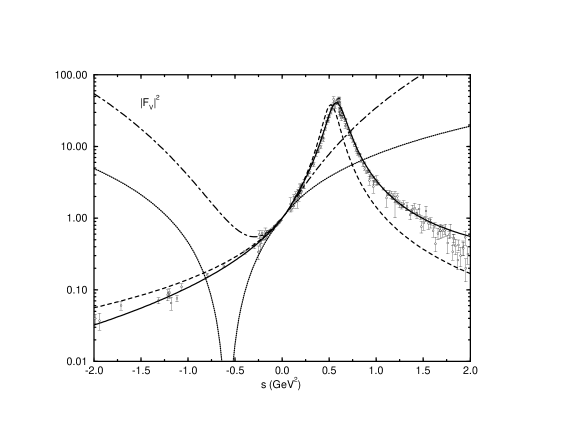
Figure 6: The pion vector form factor $\mid F\mid^{2}$ as function of $s=q^{2}$ in the space- and time-like regions. The solid line is the IAM to two loops, the dashed line the IAM to one loop, the dash-dotted line two-loop ChPT, and the dotted line one-loop ChPT.

3 Hadron Polarizabilities

The field of hadron polarizabilities was reviewed in three plenary talks at this Workshop, B. Holstein [42] reported on ChPT calculations, N.d’Hose [43] on experiments to measure the polarizabilities of the nucleon, and M. Moinester [44] on hadron polarizability experiments at Fermilab and CERN. In the Working Group, V. Olmos reported on the status of the proton polarizability and an ongoing experiment at Mainz. According to the low energy theorem [45, 46] the differential cross section for Compton scattering can be cast into the form

$$\frac{d\sigma}{d\Omega}=\left(\frac{d\sigma}{d\Omega}\right)_{P}-r_{0}(\frac{\omega^{\prime}}{\omega})^{2}\omega\omega^{\prime}\left[\frac{\alpha+\beta}{2}(1+\cos\theta)^{2}+\frac{\alpha-\beta}{2}(1-\cos\theta)^{2}\right]+...\,,$$ (11)

with $r_{0}=e^{2}/(4\pi m_{N})$ the classical proton radius. The first term on the $rhs$ of eq. (11) is the Powell cross section describing the scattering off a point particle with an anomalous magnetic moment. It can be expressed by a somewhat lengthy formula in terms of the global properties of the nucleon, its charge $Q_{N}$, mass $m_{N}$ and anomalous magnetic moment $\kappa_{N}$. The second term is of quadratic order in the photon energies $\omega$ and $\omega^{\prime}$. It contains the structure effects in the form of the electic $(\alpha)$ and magnetic $(\beta)$ polarizabilities. Fig. 7 shows the relative importance of the different contributions to the cross section. The nonrelativistic (“Thomson”) and relativistic (“Klein- Nishina”) results for scattering on an ideal point particle are quite similar but differ dramatically from the Powell cross section [47] precisely because of the anomalous magnetic moment. However, this increase of the cross section due to the anomalous magnetic moment is largely compensated by the effect of the polarizabilities and the $\pi$ pole term (Wess-Zumino-Witten term, anomaly). Of course, the anomalous magnetic moment, the polarizabilities due to excited intermediate states and the anomaly are different aspects of the same fact, namely the compositeness of the nucleon. Somehow these 3 effects conspire to give away only little information about the internal structure as contained in the terms $O(\omega^{2})$, as may be seen from the curve labeled ”LET”. The steep rise in the curve labeled ”L’vov” [48] is due to higher order terms in $\omega$, calculated by a dispersion calculation treating the $\Delta$ resonance and other high energetic effects.

The optical theorem and dispersion relations lead to Baldin’s sum rule [49],

$$\alpha_{p}+\beta_{p}=\frac{1}{2\pi^{2}}\int^{\infty}_{thr}\frac{\sigma_{tot}(\omega)}{\omega^{2}}d\omega=(14.2\pm 0.5)10^{-4}fm^{3},$$ (12)

i.e. the sum of the two polarizabilities is well determined by the total photoabsorption cross section $\sigma_{tot}$. As may be seen from eq. (11), the sum of the polarizabilities enters for forward scattering $(\theta=0)$ , the difference for backward scattering $(\theta=\pi)$, and for $\theta=\pi/2$ only $\alpha$ contributes. In spite of considerable experimental efforts, $\alpha$ and $\beta$ have not yet been determined independently by Compton scattering to a good accuracy. The present result (in units of $10^{-4}fm^{3})$ is mostly due to the work of the Illinois/SAL collaboration [50, 51], $\alpha_{p}=12.1\pm 0.8\pm 0.5$, $\beta_{p}=2.1\mp 0.8\mp 0.5$, the change of signs indicating that Baldin’s sum rule has been used as a constraint.

Figure 7: Differential cross section for Compton scattering off the proton at $\theta=90^{\circ}$. See text

The experiment reported by V. Olmos was performed with tagged photons from the Glasgow Tagger [52] at the minimum available electron energy from MAMI, i.e. 180 MeV. With this setup photon energies between 25 and 167 MeV could be tagged with an energy resolution of 0.5 MeV and a tagging efficiency of about 20%  . The scattered photons were detected with the TAPS photon spectrometer [53] consisting of 384 $BaF_{2}$ crystals plus plastic anti-charged particle detectors. The TAPS-tagger time resolution is 1.4 ns FWHM. The energy resolution of TAPS is 14.5 MeV. TAPS allowed to measure at polar angles between $25^{\circ}$ and $165^{\circ}$. Due to the strong collimation and the smallness of the cross section to be measured, there are backgrounds from electromagnetic processes at the collimators. These give an important contribution at low energies (25–50 MeV) and small angles ($25^{\circ}-60^{\circ}$). Other sources of background are cosmic rays that lead to random coincidences with the tagger. In this case a suppression is possible with a time cut. The recently taken Mainz data are now being analyzed with the promise to determine $\alpha_{p}$ and $\beta_{p}$ independently with an error bar of $10^{-4}fm^{3}$.

Information on the neutron is much more difficult to obtain. While a value $\alpha_{n}=(12.0\pm 1.5\pm 2.0)$ was reported from neutron scattering off heavy nuclei [54], a more recent investigation comes to a completely different result with large error bars, $\alpha_{n}=(0\pm 5)$ [55]. The problem with Compton scattering is that the Thomson term, and hence its interference with the polarizability term, vanishes for the neutron. Therefore the leading neutron contribution at low energies, $\sigma_{n}\sim(\alpha_{n}\omega^{2})^{2}$, is difficult to disentangle from the much larger proton contributions in nuclei. Though there have been efforts to determine $\alpha_{n}$ in quasifree kinematics [56], the effects of final state interactions and meson exchange currents have to be carefully analyzed.

As an alternative D. Hornidge presented data on a recent Saskatoon experiment on coherent photon scattering off the deuteron. The experimental difficulty arises from the necessity of resolving the elastic peak from the inelastic contribution. Up to now, there was only one measurement on this reaction (at Illinois [57] below 70 MeV). Using the photon tagging spectrometer and the high resolution Boston University NaI detector at the Saskatchewan Accelerator Laboratory (SAL), a measurement of elastic photon scattering from deuterium was accomplished. Tagged photons in the energy range $E_{\gamma}=$ 84.2 - 104.5 MeV were scattered from a liquid deuterium target and preliminary differential cross sections were measured at five angles covering the range $\theta_{\gamma^{\prime}}=35^{\circ}-150^{\circ}$. In a somewhat symbolical way, the cross section for this reaction is $\sigma_{d}\sim(f_{p,Th}-\alpha_{p}\omega^{2}-\alpha_{n}\omega^{2})^{2}$, i.e. the isoscalar sum $\alpha_{p}+\alpha_{n}$ interferes with the Thomson term of the proton, leading to a considerable enhancement of the neutron effect. However, the analysis would still require a more rigorous calculation of meson exchange and isobar currents in the deuteron, in order to obtain precise values for the neutron’s polarizabilities. Complex calculations by Levchuk [58] and Wilbois [59] attempt to explain these effects. The statistics of this SAL measurement are such that the errors in the differential cross sections are small enough (5 % - 10 %) to show that neither the Levchuk calculation (with a wide range of polarizabilities) nor the Wilbois calculation agree with the preliminary data.

By means of polarization experiments it will be possible to also measure the 4 spin (or vector) polarizabilities of the proton. As shown by T. Hemmert, the amplitude for Compton scattering off a proton $(\;\gamma\;p\rightarrow\gamma^{\prime}\;p^{\prime}\;)$ can be written in terms of 6 structure functions $A_{i}(\omega,\theta)$,

$$T = A_{1}(\omega,\theta)\;\vec{\epsilon}^{*\prime}\cdot\vec{\epsilon}+A_{2}(\omega,\theta)\;\vec{\epsilon}^{*\prime}\cdot\hat{k}\;\vec{\epsilon}\cdot\hat{k}^{\prime}+A_{3}(\omega,\theta)\;i\vec{\sigma}\cdot(\vec{\epsilon}^{*\prime}\times\vec{\epsilon})$$

$$+A_{4}(\omega,\theta)\;i\vec{\sigma}\cdot(\hat{k}^{\prime}\times\hat{k})\vec{\epsilon}^{*\prime}\cdot\vec{\epsilon}+A_{5}(\omega,\theta)\;i\vec{\sigma}\cdot[(\vec{\epsilon}^{*\prime}\times\hat{k})\vec{\epsilon}\cdot\hat{k}^{\prime}-(\vec{\epsilon}\times\hat{k}^{\prime})\vec{\epsilon}^{*\prime}\cdot\hat{k}]$$

$$+A_{6}(\omega,\theta)\;i\vec{\sigma}\cdot[(\vec{\epsilon}^{*\prime}\times\hat{k}^{\prime})\hat{\epsilon}\cdot\hat{k}^{\prime}-(\vec{\epsilon}\times\hat{k})\vec{\epsilon}^{*\prime}\cdot\hat{k}].$$

Here $\vec{\epsilon},\hat{k}\;(\vec{\epsilon}^{\prime},\hat{k}^{\prime})$ are the polarization vector and the direction of the incident (final) photon, while $\vec{\sigma}$ denotes the spin vector of the nucleon. The structure-dependent polarizabilities are of relative order $\omega$ with regard to the leading terms of a Taylor series in $\omega$,

$$A_{1}(\omega,\theta) = -\frac{e^{2}}{m_{p}}+4\pi\left(\alpha+\cos\theta\right)\omega^{2}-\frac{e^{2}}{4m_{p}^{3}}\left(1-\cos\theta\right)\omega^{2}+\ldots$$

$$A_{2}(\omega,\theta) = \frac{e^{2}}{m_{p}^{2}}\omega-4\pi\beta\omega^{2}+\ldots$$

$$A_{3}(\omega,\theta) = \left[1+2\kappa_{p}-(1+\kappa_{p})^{2}\cos\theta\right]\frac{e^{2}}{2m_{p}^{2}}\omega-\frac{(2\kappa_{p}+1)e^{2}}{8m_{p}^{4}}\cos\theta\;\omega^{3}$$

$$+4\pi\left[\gamma_{1}-(\gamma_{2}+2\gamma_{4})\cos\theta\right]\omega^{3}+\ldots$$

$$A_{4}(\omega,\theta) = -\frac{(1+\kappa_{p})^{2}e^{2}}{m_{p}^{2}}\omega+4\pi\gamma_{2}\omega^{3}+\ldots$$

$$A_{5}(\omega,\theta) = \frac{(1+\kappa_{p})^{2}e^{2}}{2m_{p}^{2}}\omega+4\pi\gamma_{4}\omega^{3}+\ldots$$

$$A_{6}(\omega,\theta) = -\frac{(1+\kappa_{p})e^{2}}{2m_{p}^{2}}\omega+4\pi\gamma_{3}\omega^{3}+\ldots,$$ (14)

which defines the scalar polarizabilities $\alpha$ and $\beta$, and the vector polarizabilities $\gamma_{1}$, $\gamma_{2}$, $\gamma_{3}$ and $\gamma_{4}$ of the proton. The latter were calculated by Bernard et al. [60] in HBChPT at $O(p^{3})$. Hemmert et al. [61] have now explicitly included $\Delta$ degrees of freedom in an expansion to $O(\epsilon^{3})$, where $\epsilon$ denotes an external momentum, a quark mass, or the N-$\Delta$ mass splitting. The calculation includes the anomaly, $\Delta$ pole terms and both N-$\pi$ and $\Delta-\pi$ loops, whose contributions are shown in Tab. 1.

	$N\pi$	WZW	$\Delta$	$\Delta\pi$	$O(\epsilon^{3})$	$O(p^{3})$	“experiment”
$\gamma_{1}$	$+4.6$	$-22.0$	$0$	$-0.21$	$-17.6$	$-17.4$
$\gamma_{2}$	$+2.3$	$0$	$-2.4$	$-0.23$	$-0.3$	$+2.3$
$\gamma_{3}$	$+1.2$	$+11.0$	$0$	$-0.12$	$+12.1$	$+12.2$
$\gamma_{4}$	$-1.2$	$-11.0$	$+2.4$	$+0.12$	$-9.7$	$-12.2$
$\gamma_{0}$	$+4.7$	$0$	$-2.4$	$-0.2$	$+2.0$	$4.7$	$-1.34$
$\gamma_{\pi}$	$+4.5$	$-44.0$	$+2.4$	$-0.2$	$-37.2$	$-39.5$	$-(27.6\pm 1.9\pm 3.2)$

Table 1: The vector polarizabilities of the proton as calculated in HBChPT to $O(\epsilon^{3})$ by Hemmert et al. [61] and to $O(p^{3})$ by Bernard et al. [60]. For the individual contributions see the text. The results are given in units of $10^{-4}\;fm^{4}$.

Is is seen from the table that the anomaly (Wess-Zumino-Witten term, WZW) dominates 3 of the vector polarizabilities. Only the numerically small $\gamma_{2}$ is free of a WZW contribution. In this case the N$\pi$ loops are predicted to be canceled by $\Delta$ contributions, leading to a change of sign in the net result. Also the value of $\gamma_{4}$ is very sensitive to $\Delta$ degrees of freedom. The forward scattering amplitude is determined by the structure functions $A_{1}$ and $A_{3}$ (see eq. (13)). According to eq. (14) the spin-independent cross section is then a function of $\alpha+\beta$, while the spin-dependent one measures the combination $\gamma_{1}-\gamma_{2}-2\gamma_{4}=\gamma_{0}$. The former combination is known from Baldin’s sum rule, the latter one is related to an integral over the difference of the absorption cross sections for the helicity states 3/2 and 1/2, similar to the Gerasimov-Drell-Hearn sum rule (GDH), but weighted with an additional $\omega^{-2}$. As may be seen in Tab. 1, the experimental value [62] differs from the predictions even in sign. While the forward spin polarizability $\gamma_{0}$ is small and independent of the anomaly, the backward spin polarizability $\gamma_{\pi}=\gamma_{1}+\gamma_{2}+2\gamma_{4}$ (see eq. (14)!) is very large, essentially because of the anomaly contribution. The corresponding experimental value as estimated by a multipole analysis [63] is shown in Tab. 1 and compared to the predictions. When comparing theory and experiment, it has to be kept in mind that the data were determined indirectly from a multipole analysis and/or extrapolation of unpolarized photon scattering. The full set of spin polarizabilities could be extracted by scattering circularly polarized photons off polarized nucleons, which will be another important test of low energy QCD and ChPT. On the theoretical side it will be necessary to study $O(\epsilon^{4})$ corrections to the results given in Tab. 1 in order to check the convergence of the perturbation series.

Concerning a somewhat related object, A. L’vov reported on a test of the GDH [64], which relates a weighted integral of the spin-dependent photoabsorption cross section $\Delta\sigma=\sigma_{3/2}-\sigma_{1/2}$ to the anomalous magnetic moment of the nucleon. A failure to saturate the GDH for the isospin-odd channel may imply [62, 65] either a large cross section $\Delta\sigma(\gamma n)\simeq-\Delta\sigma(\gamma p)\sim 50\,\mu$b in the few-GeV energy region or, alternatively, a violation of the Vector Meson Dominance for the spin-dependent transitions at high energies. Presently, an experiment at Mainz is scheduled to measure $\Delta\sigma(\gamma p)$ up to 800 MeV using a large $4\pi$ detector. Further measurements up to a few GeV will be necessary to establish whether the GDH integral converges to its canonical value.

It was proposed [65] to determine the forward Compton scattering amplitude,

$$f(\omega)=\vec{\epsilon}^{\;\prime}\!\cdot\vec{\epsilon}\,f_{1}(\omega)+i\omega\vec{\sigma}\cdot\vec{\epsilon}^{\;\prime}\!\times\vec{\epsilon}\,f_{2}(\omega),$$ (15)

from the reaction $\gamma p\to e^{+}e^{-}p$ by studying the interference between the Bethe-Heitler (BH) and the virtual Compton Scattering (VCS) amplitudes of the reaction. Since the BH mechanism produces $e^{+}e^{-}$ pairs in states of positive C-parity and the VCS gives C-odd pairs, such an interference results in an asymmetry between $e^{+}$- and $e^{-}$-yields in the same kinematics. In the regime where the transverse momentum $Q$ of the pair and its invariant mass $M_{e^{+}e^{-}}$ are small, the VCS amplitude is determined by the same functions $f_{1}$ and $f_{2}$ which describe the forward real Compton scattering. The corresponding asymmetry [65],

$$\Sigma(e^{+}/e^{-}) \sim -\frac{137\,Q^{3}}{\omega M_{e^{+}e^{-}}}\Big{\{}(\mbox{\,Re\,}f_{1}(\omega)-h_{\gamma}h_{N}\omega\mbox{\,Re\,}f_{2}(\omega))\cos\phi$$ (16)

$$\hskip 40.00006pt{}+(-h_{\gamma}\mbox{\,Im\,}f_{1}(\omega)+h_{N}\omega\mbox{\,Im\,}f_{2}(\omega))\sin\phi\Big{\}},$$

depends on the photon helicities $h_{\gamma}=\pm 1$ and the proton spin projections $\frac{1}{2}h_{N}=\pm\frac{1}{2}$ upon the beam direction and determines a preferred azimuthal orientation $\phi$ of the pair (i.e. the $e^{+}{-}e^{-}$ plane) with respect to its transverse momentum $\vec{Q}$. Measuring the asymmetry $\Sigma(e^{+}/e^{-})$ on a polarized target, one can find the imaginary part of $f_{2}$ and hence $\Delta\sigma=-8\pi\mbox{\,Im\,}f_{2}$, according to unitarity. Moreover, with circularly polarized photons one can also find $\mbox{\,Re\,}f_{2}$, which is related to $\mbox{\,Im\,}f_{2}$ by a dispersion relation and gives further constraints for $\mbox{\,Im\,}f_{2}$. Since the GDH sum rule is valid if and only if the function $f_{2}$ vanishes at high energies, direct measurements of $f_{2}$ in the reaction $\gamma p\to e^{+}e^{-}p$ at a few GeV could serve as a sensitive test of the GDH sum rule.

Our present knowledge about the pion polarizability is even more unsatisfactory than in the case of the nucleon. In the past, information has been obtained from radiative pion scattering off heavy nuclei at Serpukhov $(\alpha_{\pi\pm}=6.8\pm 1.4\pm 1.2)$, from radiative pion photoproduction $\gamma p\rightarrow\gamma\pi^{+}n$ at the Lebedev Institute with the result $20\pm 12$, and from various evaluations of the reaction $\gamma\gamma\rightarrow\pi^{+}\pi^{-}$. The latter results are quite sensitive to badly known off-shell effects and lead to a wide range of predictions. The value of the polarizability derived from radiative pion photoproduction [66] has very large error bars and is at variance with ChPT. It has therefore been proposed to repeat this experiment at MAMI.

The differential cross section of elastic $\gamma\pi^{+}$ scattering and the difference of the polarizabilities $\alpha_{\pi^{+}}-\beta_{\pi^{+}}$ can be found by extrapolating the experimental data on radiative pion photoproduction to the pion pole [66, 67]. An appropriate kinematics for the experiment was suggested [68] in order to increase the contribution of the polarizability in the physical region, to avoid additional singularities close to the region of extrapolation and to separate the signal from the background processes. The calculation takes account of the $P_{33}(1232)$ and $P_{11}(1440)$ resonances and shows that in the suggested kinematical region the contribution of resonances should be under control. As a result of extrapolation at fixed $s_{1}$ (energy of the pion-photon final state), should not depend on the incident photon energy $\nu_{1}$, which can be used to check the correctness of the extrapolation procedure. The simultaneous analysis for all values of $s_{1}$ and $\nu_{1}$ collects information from the full physical region and decreases the error obtained by the extrapolation procedure. For the triple coincidences and an exposition time of 60 days, the precision is expected to be $\Delta\alpha_{\pi_{+}}=1.3$.

4 Virtual Compton Scattering

The process of virtual Compton scattering (VCS) off the proton can be observed by the reactions $e^{-}p\rightarrow e^{-}p\gamma$ and $\gamma p\rightarrow pe^{+}e^{-}$. In both cases, there appears a strong background of BH scattering together with the VCS signal. In the case of pair production the intermediate photon is time-like $(q^{2}>0)$, at low energies this process determines the polarizability of the nucleon in the time-like region. A possible application of this reaction in the limit of $q^{2}\rightarrow 0$ to test the GDH sum rule, was discussed above. In the following we will only address radiative electron scattering, which tests the polarizability in the space-like region $(q^{2}<0)$.

At low energies the amplitude can be expanded in a power series in $\omega^{\prime}$, the energy of the emitted photon. The terms in $(\omega^{\prime})^{-1}$ and $(\omega^{\prime})^{0}$ may be expressed by the global properties of the nucleon, i.e. charge, mass, anomalous magnetic moment and the elastic form factors $G_{E}$ and $G_{M}$ [69]. The higher terms depend on the internal structure of the nucleon. To leading order in $\omega^{\prime}$, there appear 10 generalized polarizabilities (GPs), as was shown by Guichon [70]. The restriction to terms linear in $\omega^{\prime}$ corresponds to the dipole approximation, i.e. the outgoing real photons have $E1$ or $M1$ radiation. The selection rules of parity and angular momentum then result in 10 GPs, 3 scalar and 7 vector (or spin) polarizabilities. However, the additional constraint of $C$ parity and nucleon crossing symmetry reduces this number to 6 independent GPs to that order, 2 scalar and 4 vector ones [71, 72, 73].

S. Scherer reported on a calculation of the GPs within the heavy-baryon formulation of chiral perturbation theory (HBChPT) to third order in the external momenta. At $O(p^{3})$, contributions to the GPs are generated by nine one-loop diagrams and the $\pi^{0}$-exchange $t$-channel pole graph [74]. For the loop diagrams only the leading-order Lagrangians, $\widehat{\cal L}_{\pi N}^{(1)}$ and ${\cal{L}}_{\pi\pi}^{(2)}$ are needed [76]. The $\pi^{0}$-exchange diagram involves the $\pi^{0}\gamma\gamma^{\ast}$ vertex provided by the Wess-Zumino-Witten Lagrangian. Some numerical results for the GPs are shown in Fig. 8. At $O(p^{3})$, the results only depend on the pion mass $m_{\pi}$, the axial coupling constant $g_{A}$, and the pion decay constant $F_{\pi}$.

Figure 8: Generalized polarizabilities of the proton. Solid line: calculation with the linear sigma model [71], dashed line: constituent quark model [70], dash-dotted line: HBChPT [74], dotted line: effective lagrangian model [75]. The results of the quark model have been scaled.

For example, the prediction for the generalized electric polarizability of the proton,

$$\frac{\alpha_{p}({q}^{2})}{\alpha_{p}(0)}=1-\frac{7}{50}\frac{q^{2}}{m^{2}_{\pi}}+\frac{81}{2800}\frac{q^{4}}{m^{4}_{\pi}}+O\left(\frac{q^{6}}{m^{6}_{\pi}}\right),\,\,\alpha_{p}=\frac{5e^{2}g_{A}^{2}}{384\pi^{2}m_{\pi}F_{\pi}^{2}}=12.8\times 10^{-4}\,\mbox{fm}^{3},$$

decreases considerably faster with $q^{2}$ than in the constituent quark model [70]. The predictions for the spin-dependent GPs originate from two rather distinct sources—an isoscalar piece from pionic loop contributions, and an isovector piece from the $\pi^{0}$ exchange diagram contributing to the spin-dependent GPs only. The loop contribution to the spin-dependent GPs is generally much smaller than the the $\pi^{0}$-exchange contribution. For example, the spin-dependent GP $P^{(11,11)1}$ is given by

$$P^{(11,11)1}(q^{2})=-\frac{1}{288}\frac{g_{A}^{2}}{F_{\pi}^{2}}\frac{1}{\pi^{2}M}\left[\frac{q^{2}}{m^{2}_{\pi}}-\frac{1}{10}\frac{q^{4}}{m^{4}_{\pi}}\right]+\frac{1}{3M}\frac{g_{A}}{8\pi^{2}F^{2}_{\pi}}\tau_{3}\left[\frac{q^{2}}{m^{2}_{\pi}}-\frac{q^{4}}{m^{4}_{\pi}}\right]+O\left(\frac{q^{6}}{m^{6}_{\pi}}\right),$$

and vanishes at the origin as a consequence of $C$ invariance [73]. This is not true for the prediction in the constituent quark model [70]. It is also worthwhile pointing out that for 5 of the 7 vector GPs, HBChPT results in much larger values than in the case of the quark model.

According to Guichon [70], the GPs are denoted by $P^{(\rho^{\prime}L^{\prime},\rho L)S}$, with $\rho=$0,1 and 2 for Coulomb, magnetic and electric multipoles, and $L$ standing for the multipolarities. The superscript $S$ can take the values 0 (scalar GPs) and 1 (vector or spin GPs). Since the electric $(\rho=2)$ and Coulomb $(\rho=0)$ multipoles are related in the low energy limit by gauge invariance (Siegert’s theorem), Guichon expressed the electric transitions $(\rho=2)$ by the Coulomb $(\rho=0)$ ones plus a remainder, which leads to so-called mixed multipoles $\hat{P}^{(\rho^{\prime}L^{\prime},L)S}$. A. Metz explained in detail how the 10 GPs defined in this way are related among themselves and with the polarizabilities for real photons obtained at $q=0$ [72, 73]. In particular, the 3 scalar GPs $P^{(01,01)0},P^{(11,11)0}$ and $\hat{P}^{(01,0)0}$ are related such that $\hat{P}^{(01,0)0}$ can be eliminated. In the real photon limit, $q\rightarrow 0,P^{(01,01)0}\sim\alpha$ and $P^{(11,11)0}\sim\beta$. At finite $q$, these GPs probe $\alpha(q^{2})$ and $\beta(q^{2})$, which are related to the spatial distributions of the electric and magnetic dipole moments in the nucleon.

The 7 vector GPs $P^{(01,01)1},P^{(11,11)1},P^{(11,00)1},P^{(01,12)1},P^{(11,02)1},\hat{P}^{(11,2)1}$ and $\hat{P}^{(01,1)1}$ are related by 3 equations such that the 2 ”mixed” GPs and one further GP can be eliminated. In the limit of $q\rightarrow 0,\;P^{(01,12)1}\sim\gamma_{3}$ and $P^{(11,02)1}\sim(\gamma_{2}+\gamma_{4})$, describing the Coulomb dipole/magnetic quadrupole and Coulomb quadrupole/magnetic dipole interferences, respectively. The other 3 GPs, corresponding to $C1/C1,M1/M1$ and $M1/C0$ radiation in order, vanish in the limit $q\rightarrow 0$.

A. Metz further reported on calculations of the GPs in the linear sigma model (LSM) [71]. Since this model fulfills all the necessary symmetry relations and because of its simplicity, the relations between the GPs were first found in the framework of that model. In fact, the leading terms of the polarizabilities in a power series expansion in $\mu=m_{\pi}/m_{N}$ agree with the heavy baryon ChPT [74].

In the differential cross section for unpolarized particles, the interference term between BH and VCS contains 4 structure functions $P_{LL},P_{TT},P_{LT}$ and $P^{\prime}_{LT}$, which can be separated by a super-Rosenbluth plot. Due to the relations between the GPs, however, the latter two functions are equivalent up to a kinematical factor. Therefore, such an experiment will provide information on 3 (combinations) of GPs only. As was recently shown by M. Vanderhaeghen [78], the additional information may be obtained in the reaction $p(\vec{e},e^{\prime}\vec{p})\gamma$, by measuring the asymmetries for different directions of the recoil nucleon polarization. This would lead to 3 further structure functions $P^{z}_{LT},P^{{}^{\prime}z}_{LT},P^{{}^{\prime}x}_{LT}$, with $x$ and $z$ corresponding to nucleon polarization in the hadronic plane, perpendicular and parallel to the virtual photon, respectively. In the calculation of Metz, the GPs lead to a decrease of the cross section for a typical MAMI kinematics by about $2-10\%$, increasing with $\omega^{\prime}$. In the case of the asymmetries, the effect of the GPs can have both signs, with a somewhat smaller absolute value $(2-6\%)$. In view of the unexpectedly large radiative corrections and the smallness of the effects, a full Rosenbluth separation will be quite a challenge.

VCS is presently being investigated at MIT-Bates (proposal 97-03), MAMI (collaboration A1) and Jefferson Lab [43]. It is the aim of the former two experiments to measure the GPs of the proton, while there are also proposals to study the resonance region and the quark distribution of the nucleon at Jefferson Lab.

R. Miskimen reported on the Bates proposal which has been optimized for measurements of $\alpha(q)$ and $\beta(q)$ at low momentum transfer. The scattered protons will be detected in a cluster of three OOPS modules (Out-Of-Plane-Spectrometers), two of which will be placed out of the scattering plane. Out-of-plane detection is an important capability for VCS experiments. By going above or below the scattering plane, the BH process can be suppressed relative to VCS because one can move away from the direction of the incident and scattered electrons. By going out of plane it is also possible to reach low values of momentum transfer, where the kinematical focussing of the proton weakens. Clearly data at low momentum transfer are needed in order to test ChPT.

Data will be simultaneously taken using three OOPS modules at 3 combinations of scattering angles, $(\theta,\phi)=(90^{\circ},90^{\circ}),(90^{\circ},270^{\circ})$, and $(90^{\circ},180^{\circ})$. For the first two kinematical conditions the experiment is sensitive to $(\epsilon P_{LL}-P_{TT})$, in the last case also $P_{LT}$ is being probed. Data will be taken with $\epsilon=0.9$ to maximize the sensitivity to $P_{LL}$, which is proportional to $\alpha(q)$. The initial photon momentum will be 240 MeV, or $Q^{2}\approx 0.05GeV^{2}$, which is in the anticipated range of validity of chiral perturbation theory. Because the electron scattering virtual photon flux factor is approximately 100 times larger than typical real photon tagging rates, the extracted polarizabilities should have greatly reduced statistical uncertainty compared to the real Compton scattering case. Taking VCS data simultaneously will also reduce the systematic errors of the experiment.

J. Roche presented some preliminary results of the VCS collaboration at MAMI. Data have been taken in the scattering plane at $Q^{2}=0.33GeV^{2}$ and virtual photon polarization $\epsilon=0.62$. As is shown in Fig. 9, forward scattering is completely dominated by the BH process such that VCS can only be studied under backward angles. The prediction of the low energy expansion (full curve in Fig. 9) is verified within a precision of $10\%$. It includes the BH background, the Born terms and radiative corrections to BH scattering. The size of the radiative corrections turned out to be quite large, it is of the order of the structure effects to be measured. At the low final photon energy $(\omega^{\prime}=q^{\prime}=45MeV)$, such effects of the GPs will be very small, while $10-15\%$ effects are expected at larger energies, e.g. $\omega^{\prime}=90MeV$. The goal of the experiments is to reach statistical and systematical errors of less than $3\%$. In order to achieve this accuracy further improvements are necessary with regard to the stability between the runs and the global normalization of the data. However, this pilot experiment has clearly demonstrated that measurements of the GPs are within reach. Concerning the necessary accuracy of the data, it should be kept in mind that the dependence of the GPs on the momentum transfer $Q^{2}$ is predicted quite differently in various models. In particular pion cloud contributions lead to large transition radii and GPs decreasing much more rapidly with $Q^{2}$ than in the case of quark and phenomenological models. Similarly the low energy constants introduced in ChPT correspond to point interactions, i.e. form factors are only build up by higher loop corrections. This will also be the case for the triangle anomaly (WZW term, $\pi^{\circ}$ exchange) which is responsible for the large values of some of the vector polarizibilities. The internal (spatial) structure of this term could be resolved by VCS with polarization degrees of freedom.

Figure 9: The differential cross section for virtual Compton scattering at $\omega^{\prime}=q^{\prime}=45MeV$. Preliminary results of the VCS collaboration at MAMI. See text and Ref. [43].

5 Acknowledgement

It is a pleasure to thank all the participants of the working group for their contributions and the lively discussions.

References

- [1] H.-W. Hammer, U.-G. Meißner and D. Drechsel, Phys. Lett. B 385 (1996) 343.
- [2] T. A. Armstrong et al., Phys. Rev. Lett. 70 (1993) 1212.
- [3] G. Bardin et al., Nucl. Phys. B 411 (1994) 3.
- [4] A. Antonelli et al., Phys. Lett. B 334 (1994) 431, ibid. 313 (1993) 283, and preprint submitted to Nucl. Phys.
- [5] A. Zichichi et al., Nuovo Cimento 24 (1962) 170.
- [6] P. Bosted et al., Phys. Rev. Lett. 68, 3841 (1992).
- [7] A. F. Sill et al., Phys. Rev. D 48, 29 (1993).
- [8] G. G. Simon et al., Nucl. Phys. A 333 (1980) 381.
- [9] P. Mergell, Ulf-G. Meißner, D. Drechsel, Nucl. Phys. A 596 (1996) 367.
- [10] M. Weitz et al., Phys. Rev. Lett. 72 (1994) 328; D. J. Berkeland et al., Phys. Rev. Lett. 75 (1995) 2470.
- [11] S. Kopecki et al., Phys. Rev. Lett. 74 (1995) 2427.
- [12] A. Lung et al., Phys. Rev. Lett. 70 (1993) 718.
- [13] H. Anklin et al., Phys. Lett. B 336 (1994) 313.
- [14] J. Jourdan et al., A1 collaboration at MAMI, to be published.
- [15] E. Bruins et al., Phys. Rev. Lett. 75 (1995) 21.
- [16] S. Platchkov et al., Nucl. Phys. A 510 (1990) 740.
- [17] R. G. Arnold et al., Phys. Rev. C 23 (1981) 363.
- [18] H. Arenhövel, Phys. Lett. B 199 (1987) 13; Z. Phys. A 331 (1988) 509.
- [19] F. Klein, Proc. of PANIC96, Williamsburg, USA (1996); H. Schmieden, Proc. of SPIN96, Amsterdam (1996); M. Ostrick, Ph. D. thesis in preparation, University of Mainz; C. Herberg, Ph. D. thesis in preparation, University of Mainz.
- [20] J. Becker, Ph. D. thesis, University of Mainz (1997); J. Becker et al., Proc. Conf. on Polarized Gas Targets and Polarized Beams, Urbana, USA (1997); P. Grabmayr et al., Proc. Conf. on Hadron Physics, Trieste, Italy (1997).
- [21] M. Meyerhoff et al., Phys. Lett. B 327 (1994) 201.
- [22] W. Heil (contact person), MAMI Proposal A1/4-95.
- [23] G. Höhler in Pion-Nucleon Scattering, Landoldt-Börnstein I/9b2, ed. H. Schopper, Springer Verlag, Heidelberg (1983).
- [24] J. Gasser, M.E. Sainio, A. Svarc, Nucl. Phys. B 307 (1988) 779.
- [25] V. Bernard, N. Kaiser, Ulf-G. Meißner, Nucl. Phys. A 611 (1996) 429.
- [26] G. Höhler et al., Nucl. Phys. B 114 (1976) 505; G. Höhler in Pion-Nucleon Scattering, Landoldt-Börnstein I/9b2, ed. H. Schopper, Springer (1983), sects.2.5.2 and A. 11.
- [27] I. Sabba Stefanescu, J. Math. Phys. 21 (1980) 175.
- [28] G. Höhler, N Newsletter 9 (1993) 108.
- [29] W. Grein, P. Kroll, Nucl. Phys. A 338 (1980) 332.
- [30] R. Machleidt et al., Physics Reports 149 (1987) 1.
- [31] M.E. Biagini, S. Dubnička, E. Etim, P. Kolář, Nuovo Cim. A104 (1991) 363.
- [32] S. Dubnička, A.Z. Dubničkov, and P. Stríženec, Nuovo Cim. A106 (1993) 1253.
- [33] B. Mueller et al., SAMPLE Collaboration, Phys. Rev. Lett. 78 (1997) 3824.
- [34] H.-W. Hammer, Ph.D. thesis, University of Mainz (1997).
- [35] M. J. Musolf, H.-W. Hammer and D. Drechsel, Phys. Rev. D55 (1997) 2741.
- [36] M. J. Ramsey-Musolf and H.-W. Hammer, preprint MKPH-T-97-14, [hep-ph/9705409].
- [37] H.-W. Hammer and M. J. Ramsey-Musolf, Phys. Lett. B (in print).
- [38] J. Gasser and U. G. Meißner, Nucl. Phys. B357 (1991) 90.
- [39] T. N. Truong, Phys. Rev. Lett. 61 (1988) 2526; T. Hannah, Phys. Rev. D 54 (1996) 4648.
- [40] T. Hannah, Phys. Rev. D 55 (1997) 5613.
- [41] L. V. Dung and T. N. Truong, preprint [hep-ph/9607378].
- [42] B. Holstein, ”ChPT for Hadron Polarizabilities”, Proc. of ChPT97, Mainz (1997).
- [43] N. d’Hose, ”Experiments on Nucleon Polarizablities”, Proc. of ChPT97, Mainz (1997).
- [44] M. Moinester, ”Status and Outlook of Hadron Polarizability Experiments at Fermilab and CERN”, Proc. of ChPT97, Mainz (1997).
- [45] M. Gell-Mann et al., Phys. Rev. 96 (1954) 1433; F. E. Low, Phys. Rev. 96 (1954) 1428.
- [46] V. A. Petrun’kin, Sov. J. Part. Nucl. 12 (1981) 278.
- [47] J. L. Powell, Phys. Rev. 75 (1949) 32.
- [48] A. I. L’vov, V. A. Petrun’kin and M. Schumacher, Phys. Rev. C 55 (1997) 359.
- [49] A. M. Baldin, Nucl. Phys. 18 (1960) 310.
- [50] E. L. Hallin et al., Phys. Rev. C48 (1993) 1497.
- [51] B. E. MacGibbon et al., Phys. Rev. C52 (1995) 2097.
- [52] I. Anthony et al., NIM A301 (1991) 230; S. J. Hall et al., NIM A368 (1996) 698.
- [53] R. Novotny et al., IEEE Trans. on Nucl. Science 38 (1991) 379.
- [54] J. Schmiedmayer et al., Phys. Rev. Lett. 66 (1991) 1015.
- [55] L. Koester et al., Phys. Rev. C51 (1995) 3363.
- [56] K. W. Rose et al., Nucl. Phys. A514 (1990) 621.
- [57] M. A. Lucas, Ph. D. thesis, University of Illinois at Urbana-Champaign (1994).
- [58] M. I. Levchuk and A. I. L’vov , Few-Body Systems Suppl. 9 (1995) 439.
- [59] Th. Wilbois, P. Wilhelm, H. Arenhövel, Few-Body Systems Suppl. 9 (1995) 263.
- [60] V. Bernard et al., Nucl. Phys. B388 (1992) 315.
- [61] Th. Hemmert et al., Phys. Rev. D55 (1997) 5598.
- [62] A. M. Sandorfi, C.S. Whisnant, and M. Khandaker, Phys. Rev. D 50 (1994) R6681.
- [63] J. Tonnison et al., LEGS preprint (1997).
- [64] S. B. Gerasimov, Yad. Fiz. 2 (1965) 839; S. D. Drell and A. C. Hearn, Phys. Rev. Lett. 16 (1966) 908.
- [65] A. I. L’vov et al., [nucl-th/9707006], to appear in Phys. Rev. C (1998).
- [66] T. A. Aibergenov et al., Czech.J.Phys. B36 (1986) 948.
- [67] D. Drechsel and L. Fil’kov, Z.Phys. A349 (1994) 177.
- [68] J. Ahrens et al., Few-Body Syst. Suppl. 9 (1995) 449.
- [69] S. Scherer, A. Yu. Korchin, J. H. Koch, Phys. Rev. C 54 (1996) 904.
- [70] P.A.M. Guichon, G.Q. Liu, A.W. Thomas, Nucl. Phys. A591 (1995) 606.
- [71] A. Metz and D. Drechsel, Z. Phys. A 356 (1996) 351; Z. Phys. A 359 (1997) 165.
- [72] D. Drechsel, G. Knöchlein, A. Metz, S. Scherer, Phys. Rev. C55 (1997) 424.
- [73] D. Drechsel, G. Knöchlein, A.Yu. Korchin, A. Metz, S. Scherer, [nucl-th/9704064], to appear in Phys. Rev. C (1998).
- [74] T.R. Hemmert, B.R. Holstein, G. Knöchlein, S. Scherer, Phys. Rev. D55 (1997) 2630 and Phys. Rev. Lett. 79 (1997) 22.
- [75] M. Vanderhaeghen, Phys. Lett., B 368 (1996) 13.
- [76] G. Ecker and M. Mojžiš, Phys. Lett. B365 (1996) 312.
- [77] V. Bernard et al., Nucl. Phys. B373 (1992) 346.
- [78] M. Vanderhaeghen, Phys. Lett. B402 (1997) 243.