Kaon and Hyperon Form Factors in Kaon Electroproduction on the Nucleon

Abstract

The electromagnetic form factors of strange mesons and baryons are studied by means of kaon electroproduction on the nucleon. The response functions that are sensitive to the $K^{0}$, $\Lambda$, $\Sigma^{+}$, and $KK^{*}\gamma$ transition form factors are systematically explored. The effects of these form factors on several response functions are discussed.

1 INTRODUCTION

The study of the electromagnetic structure of hadrons provides an important key for our understanding of hadronic structure, since form factors reflect the charge distribution of quarks and gluons inside the hadron. During the last decades there has been considerable effort to develop models for not only the nucleon, but also hyperon and meson form factors. Nevertheless, the main problematic issue is the lack of experimental verification of these models due to the lack of stable targets in the case of strange hadrons.

Unlike the case of the proton, where both electric and magnetic form factors [$G_{E}(q^{2})$ and $G_{M}(q^{2})$] can be extracted directly, the measurement of charged meson (e.g. $\pi^{+}$ and $K^{+}$) form factors requires an indirect technique. The method is known as Chew-Low extrapolation [1, 2] and based on the extrapolation of the electroproduction data to the pion/kaon pole, where the dominance of the longitudinal differential cross section can isolate the contribution of the pion/kaon form factor from the contamination of other diagrams. However, there is no certainty that such techniques are also applicable to other strange mesons and hyperons (e.g., $K^{0}$, $\Lambda$ and $\Sigma$), since the required experimental data are not available at the present.

In this paper, we suggest that kaon electroproduction may provide at least an indirect method for obtaining information on these form factors. The result presented here provides an extension of our previous report [3].

2 RESPONSE FUNCTIONS IN KAON ELECTROPRODUCTION

While the cross section for an experiment using unpolarized electron beams has only four individual terms (see e.g. Ref. [4]), the differential cross section for kaon production using polarized electron, target, and recoil may be written in terms of response functions as [5]

Table 1: Complete response functions for pseudoscalar meson electroproduction [5]. The polarization of the target (recoil) is indicated by $\alpha$ ($\beta$). The last three columns (${}^{c}TL^{\prime}$, ${}^{s}TL^{\prime}$, and $TT^{\prime}$) are response functions for polarized electrons. $\ddagger$ denotes a response function which does not vanish but is identical to another response function.

Note	$\beta$	$\alpha$	$T$	$L$	${}^{c}TL$	${}^{s}TL$	${}^{c}TT$	${}^{s}TT$	${}^{c}TL^{\prime}$	${}^{s}TL^{\prime}$	$TT^{\prime}$
Unpolarized	0	0	$R_{T}^{00}$	$R_{L}^{00}$	$R_{TL}^{00}$	0	$R_{TT}^{00}$	0	0	$R_{TL^{\prime}}^{00}$	0
Polarized	0	$x$	0	0	0	$R_{TL}^{0x}$	0	$R_{TT}^{0x}$	$R_{TL^{\prime}}^{0x}$	0	$R_{TT^{\prime}}^{0x}$
target	0	$y$	$R_{T}^{0y}$	$R_{L}^{0y}$	$R_{TL}^{0y}$	0	$\ddagger$	0	0	$R_{TL^{\prime}}^{0y}$	0
	0	$z$	0	0	0	$R_{TL}^{0z}$	0	$R_{TT}^{0z}$	$R_{TL^{\prime}}^{0z}$	0	$R_{TT^{\prime}}^{0z}$
Polarized	$x^{\prime}$	0	0	0	0	$R_{TL}^{x^{\prime}0}$	0	$R_{TT}^{x^{\prime}0}$	$R_{TL^{\prime}}^{x^{\prime}0}$	0	$R_{TT^{\prime}}^{x^{\prime}0}$
recoil	$y^{\prime}$	0	$R_{T}^{y^{\prime}0}$	$\ddagger$	$\ddagger$	0	$\ddagger$	0	0	$\ddagger$	0
	$z^{\prime}$	0	0	0	0	$R_{TL}^{z^{\prime}0}$	0	$R_{TT}^{z^{\prime}0}$	$R_{TL^{\prime}}^{z^{\prime}0}$	0	$R_{TT^{\prime}}^{z^{\prime}0}$
Polarized	$x^{\prime}$	$x$	$R_{T}^{x^{\prime}x}$	$R_{L}^{x^{\prime}x}$	$R_{TL}^{x^{\prime}x}$	0	$\ddagger$	0	0	$R_{TL^{\prime}}^{x^{\prime}x}$	0
target	$x^{\prime}$	$y$	0	0	0	$\ddagger$	0	$\ddagger$	$\ddagger$	0	$\ddagger$
and	$x^{\prime}$	$z$	$R_{T}^{x^{\prime}z}$	$R_{L}^{x^{\prime}z}$	$\ddagger$	0	$\ddagger$	0	0	$\ddagger$	0
recoil	$y^{\prime}$	$x$	0	0	0	$\ddagger$	0	$\ddagger$	$\ddagger$	0	$\ddagger$
	$y^{\prime}$	$y$	$\ddagger$	$\ddagger$	$\ddagger$	0	$\ddagger$	0	0	$\ddagger$	0
	$y^{\prime}$	$z$	0	0	0	$\ddagger$	0	$\ddagger$	$\ddagger$	0	$\ddagger$
	$z^{\prime}$	$x$	$R_{T}^{z^{\prime}x}$	$\ddagger$	$R_{TL}^{z^{\prime}x}$	0	$\ddagger$	0	0	$R_{TL^{\prime}}^{z^{\prime}x}$	0
	$z^{\prime}$	$y$	0	0	0	$\ddagger$	0	$\ddagger$	$\ddagger$	0	$\ddagger$
	$z^{\prime}$	$z$	$R_{T}^{z^{\prime}z}$	$\ddagger$	$\ddagger$	0	$\ddagger$	0	0	$\ddagger$	0

$$\frac{d\sigma_{v}}{d\Omega_{K}}\!\!\!\! =~{}\frac{\mid{\vec{q}}_{K}\mid}{k_{\gamma}^{\rm cm}}P_{\alpha}P_{\beta}\left\{R_{T}^{\beta\alpha}+\varepsilon_{L}R_{L}^{\beta\alpha}+\left[2\varepsilon_{L}\left(1+\varepsilon\right)\right]^{\frac{1}{2}}(^{c}\!R_{TL}^{\beta\alpha}\cos\phi_{K}+~\!{}^{s}\!R_{TL}^{\beta\alpha}\sin\phi_{K})\right.$$ (1)

$$+~{}\varepsilon(^{c}\!R_{TT}^{\beta\alpha}\cos 2\phi_{K}+~\!{}^{s}\!R_{TT}^{\beta\alpha}\sin 2\phi_{K})+h\left[2\varepsilon_{L}(1-\varepsilon)\right]^{\frac{1}{2}}(^{c}\!R_{TL^{\prime}}^{\beta\alpha}\cos\phi_{K}+~\!{}^{s}\!R_{TL^{\prime}}^{\beta\alpha}\sin\phi_{K})$$

$$\left.+~{}h(1-\varepsilon^{2})^{\frac{1}{2}}R_{TT^{\prime}}^{\beta\alpha}\right\},$$

where $P_{\alpha}=(1,P_{x},P_{y},P_{z})$ and $P_{\beta}=(1,P_{x^{\prime}},P_{y^{\prime}},P_{z^{\prime}})$ indicate the target and the recoil polarization vectors, respectively. In total, there are 36 different response functions in the electroproduction of pseudoscalar mesons as listed in Table 1, although it is not necessary to measure them all for a complete experiment.

3 THE ELEMENTARY OPERATOR

The presently existing elementary models were mostly developed from fits to experimental data by taking a number of resonances and leaving their coupling constants as free parameters. However, the limited data base permits only qualitative conclusions until now. For our purpose, we will employ the elementary models of Ref. [6] and use the methods of Ref. [7] to extend these models to the $n(e,e^{\prime}K^{0})\Lambda$ and $p(e,e^{\prime}K^{0})\Sigma^{+}$ channels. Since at present no data are available in both processes, it is impossible to test the reliability of the models in these isospin channels. Therefore, for the present we are only able to estimate the relative effects that form factors have on particular response functions.

4 THE ELECTROMAGNETIC FORM FACTORS

4.1 The $K^{0}$ Form Factor

The existence of the $K^{0}$ form factor provides one of the unique properties of the neutral kaon compared with other neutral SU(3) pseudoscalar mesons. The difference between the strange and non-strange quark masses creates a non-uniform charge distribution in the $K^{0}$. As a consequence, although its total charge is zero, the $K^{0}$ has an electric form factor. Since the mass difference is still smaller than the mass scale associated with confinement in Quantum Chromodynamics (QCD), $(m_{s}-m_{d})<\Lambda_{\rm QCD}$, it could lead to a sensitive test of phenomenological models that attempt to describe nonperturbative QCD.

In this paper we employ two relativistic quark models to calculate the $K^{0}$ form factor, the light-cone quark (LCQ) model [8] and the quark-meson vertex (QMV) model [9]. The charge form factor of $K^{0}$ can be expressed as

$$F_{K^{0}}(q) = e_{d}F_{L}(q)+e_{\bar{s}}F_{H}(q)~{},$$ (2)

where $F_{L}(q)$ and $F_{H}(q)$ are two independent form factors generated by the interaction of the photon with the light quark ($d$) of charge $e_{d}$ and with the other heavier quark (${\bar{s}}$) of charge $e_{\bar{s}}$. The results are then compared with predictions from vector meson dominance (VMD) and chiral perturbation theory (ChPT). In VMD, we assume that the photon interacts with the strange quark through the $\phi$-meson and with the $u$-and $d$- quarks through $\rho$- and $\omega$-mesons, each of them having the strength proportional to the quark charge. Using ChPT to order $p^{4}$, a parameter-free prediction for the $K^{0}$ form factor at very low $q^{2}$ can be obtained which is due entirely to one-loop diagrams without a tree-level contribution. All models are compared in Fig. 2, where the charged kaon form factor is shown for comparison.

Figure 1: The $K^{0}$ and $K^{+}$ form factors predicted by the QMV calculation (dash-dotted lines), VMD model (dashed lines), ChPT (dotted lines), and LCQ model (solid lines). The same units are used for the insert.

Figure 2: The transition form factors $K^{+}K^{*+}\gamma$ and $K^{0}K^{*0}\gamma$ as predicted by Ref. [6] (dash-dotted lines) and Ref. [12] (solid lines). The dashed line shows the elastic $K^{+}$ form factor.

Figure 3: The $\Lambda$ magnetic form factors from the HVMD model (dashed line) [10] and CQS model (dash-dotted line) [11] compared with that of the neutron (solid line). All models are scaled to the experimental $\Lambda$ magnetic moment at the photon point.

Figure 4: The $\Sigma$ form factors from the CQS model [11].

4.2 The $KK^{*}\gamma$ Transition Form Factors

Although several models for the $KK^{*}\gamma$ transition form factors have been introduced, no proposal for experimental verification has been suggested. This is in contrast to their non-strange counterparts, the $\rho\pi\gamma$ and $\omega\pi\gamma$ form factors, which are very important in meson exchange current corrections to deuteron electrodisintegration. As in the $K^{0}$ case, the transition form factors are sensitive to the mass difference between strange and non-strange quarks. Figure 2 shows the transition form factors for both the neutral and the charged case, comparing the model of Ref. [6] which uses vector meson dominance and the calculation of Ref. [12] which solves a covariant Salpeter equation for a confining plus instanton-induced interaction. Both models fall off faster than the elastic $K^{+}$ form factor which is shown for comparison. The form factor in the charged case displays a zero at $q^{2}=-2.7$ GeV², indicating a destructive interference between the light and the heavy quark contributions.

4.3 Hyperon Form Factors

Theoretical interest in the hyperon electromagnetic form factors is sparked by the question of SU(3)_F flavor symmetry breaking and the effects of explicit and hidden strangeness on electromagnetic observables. Applying SU(3)_F flavor symmetry enables predicting the hyperon form factors in vector meson dominance, quark and soliton models in terms of model parameters fixed by the nucleon data.

In Fig. 4 we compare the $\Lambda$ form factors as predicted by a hybrid vector meson dominance (HVMD) calculation [10] and the chiral quark-soliton (CQS) model [11]. The HVMD mechanism provides a smooth transition from the low-$q^{2}$ behavior predicted by vector meson dominance to the high-$q^{2}$ scaling of perturbative QCD. The key feature is the application of the universality limit of the vector meson hadronic coupling SU(3) symmetry relations. Using a direct photon coupling along with a $\phi$ and $\omega$ pole they predict the $\Lambda$ form factor, while the $\Lambda-\Sigma$ transition form factor can be obtained similarly, using a direct photon coupling and a $\rho$ pole. Theoretically, the ratio of these form factors would be interesting since the $\Lambda$ form factor depends only on isoscalar currents while the $\Lambda-\Sigma$ transition depends only on isovector contributions. Hence, as pointed out in Ref. [10], this ratio might see explicit strangeness and OZI effects such as the suppression or enhancement of effective $\rho$, $\omega$ and $\phi$ vector meson-hyperon couplings relative to the vector meson-nucleon couplings and SU(3) flavor symmetry predictions.

The CQS (Nambu-Jona-Lasinio soliton) model is based on the nonlinear effective chiral-quark model, in which the quarks interact with a self-consistently generated background Goldstone field. The model can properly describe the low energy pion dynamics and can be derived from QCD by means of the instanton liquid model.

For comparison, in Fig. 4, we also show the neutron magnetic form factor with a simple, standard dipole parametrization, which were mostly used in the previous $(e,e^{\prime}K)$ studies, provided it is scaled by the $\Lambda$ magnetic moment to give the proper $\gamma\Lambda\Lambda$ vertex at the photon point. The CQS model exhibits a dipole-like form factor, while the HVMD model slightly increases at small momentum transfers before falling off as a function of $-q^{2}$ for higher momentum transfers.

Figure 4 displays the $\Sigma$ form factors as predicted by the CQS model [11]. We note that the charged $\Sigma$ form factors show a dipole behavior, as in the case of the proton. For the sake of simplicity, we will only investigate the sensitivity of response functions to the $\Sigma^{+}$ form factor.

5 RESULTS AND DISCUSSIONS

Table 2 displays the response functions that show a sensitivity of at least 10% to the $K^{0}$, $K^{+}K^{+*}$, $K^{0}K^{0*}$, $\Lambda$, and $\Sigma^{+}$ form factors for certain kinematics. No sensitivity is shown for the response functions involving triple polarization, since they are too small to be detected, about two order of magnitude smaller than the other response functions. Since there are many sensitive response functions, we will only focus on the most suitable ones with regard to experimental aspects and proposals.

Table 2: Response functions in Table 1 which are sensitive to different form factors. The elementary model is due to Ref. [6]. The sensitivities to the $K^{0}$, $K^{+}K^{+*}$, $K^{0}K^{0*}$, $\Lambda$, and $\Sigma^{+}$ form factors are denoted by $\circ$, $\bullet$, $\star$, $\diamond$, and $\ast$ , respectively, using the $K^{0}\Lambda$, $K^{+}\Sigma^{0}$, $K^{0}\Sigma^{+}$, $K^{+}\Lambda$, and $K^{0}\Sigma^{+}$ electroproduction reactions, respectively.

Note	$\beta$	$\alpha$	$T$	$L$	${}^{c}TL$	${}^{s}TL$	${}^{c}TT$	${}^{s}TT$	${}^{c}TL^{\prime}$	${}^{s}TL^{\prime}$	$TT^{\prime}$
Unpol.	0	0	$\bullet\star\diamond\ast$	$\circ\bullet\diamond\ast$	$\circ\star\diamond\ast$	.	$\star\diamond\ast$	.	.	.	.
Pol.	0	$x$	.	.	.	$\ast$	.	.	$\circ\bullet\star\diamond\ast$	.	$\bullet\star\diamond\ast$
target	0	$y$	$\star$	.	$\ast$	.	.	.	.	$\circ\bullet\diamond\ast$	.
	0	$z$	.	.	.	.	.	$\star$	$\circ\bullet\star\diamond\ast$	.	$\bullet\star\diamond\ast$
Pol.	$x^{\prime}$	0	.	.	.	.	.	$\star$	$\circ\bullet\star\diamond\ast$	.	$\bullet\star\diamond\ast$
recoil	$z^{\prime}$	0	.	.	.	.	.	.	$\circ\star\diamond\ast$	.	$\bullet\star\diamond\ast$
Pol.	$x^{\prime}$	$x$	$\bullet\star\diamond\ast$	$\circ\bullet\diamond\ast$	$\circ\diamond$	.	.	.	.	.	.
target	$x^{\prime}$	$z$	$\star\diamond$	$\diamond\ast$	.	.	.	.	.	.	.
and	$z^{\prime}$	$x$	$\star\diamond\ast$	.	$\circ\bullet\diamond$	.	.	.	.	.	.
recoil	$z^{\prime}$	$z$	$\bullet\star\diamond\ast$	.	.	.	.	.	.	.	.

Figure 5: The longitudinal and longitudi- nal-transverse response functions for the $n(e,e^{\prime}K^{0})\Lambda$ process. The solid line shows the calculation with a $K^{0}$ form factor obtained in the LCQ model while the dash-dotted line was obtained using the QMV model. The dashed line shows a computation with the $K^{0}$ pole excluded.

Figure 6: As in Fig. 6, but for different kinematics.

Table 2 can tell us, which response function is suitable for measuring a certain form factor, while the contaminations from other form factors can be minimized.

The longitudinal and transverse response functions of the $n(e,e^{\prime}K^{0})\Lambda$ reaction using two different quark models for the $K^{0}$ form factor are shown in Fig. 6 and Fig. 6. We found that the transverse response functions are insensitive to the $K^{0}$ pole as shown in Table 2. The longitudinal response functions calculated with the form factor obtained from the LCQ-model is almost 50$\%$ larger than the calculation with no $K^{0}$ pole, while the QMV-model calculation lies between those two. Similar sensitivities of the $L$ and $TL$ response functions indicate that a Rosenbluth separation is not imperative in order to isolate the $K^{0}$ form factor effects.

Figure 7: The sensitivity of response functions to different $K^{0}K^{*0}\gamma$ form factors. The solid (dash-dotted) line is obtained using the model of Ref. [12] ([6]).

Figure 8: As in Fig. 8, but for the $K^{+}K^{*+}\gamma$ form factors.

Figures 8 and 8 show the sensitivity of different transverse response functions to the neutral and charged kaon transition form factors. Since the small size of the $g_{K\Sigma N}$ coupling constant suppresses the Born terms, the $p(e,e^{\prime}K^{+})\Sigma^{0}$ reaction is used to study the $K^{+}K^{*+}\gamma$ form factor while the $p(e,e^{\prime}K^{0})\Sigma^{+}$ is sensitive to the neutral transition. Questions remain regarding additional $t$-channel resonance contributions from states like the $K_{1}$(1270) which would have a different transition form factor. The observables displayed can clearly distinguish between the different models, with the model of Ref. [12] leading to a much faster fall-off. Unfortunately, the zero in the charged transition form factor around $q^{2}=-2.6$ GeV² is not visible since the response functions are already very small at this kinematics. The large differences shown by the $T$ response function indicate that the unpolarized experiment would be able to distinguish the models once we had a reliable elementary production model.

Figure 9: The sensitivity of response functions to different $\Lambda$ form factors, the HVMD model (solid lines) [10] and the CQS model (dashed lines) [11].

Figure 10: As in Fig. 10, but for different kinematics.

In Fig. 10 and 10 we show double polarization response functions for the $p(e,e^{\prime}K^{+})\Lambda$ reaction that involve both beam and recoil polarizations. Since the $\Lambda$ form factor is multiplied by the large hadronic coupling constant $g_{K\Lambda N}$, the $p(e,e^{\prime}K^{+})\Lambda$ channel is well suited to extract this form factor. The $TT^{\prime}$ and $TL^{\prime}$ observables were subject of a recent TJNAF proposal [13]. While the $TT^{\prime}$ response function shows moderate sensitivity to the different $\Lambda$ form factors for all momentum transfers, the $TL^{\prime}$ structure function displays large sensitivities for most of the momentum transfer range shown in Fig. 10 and the entire angular range, shown in Fig. 10. The $TT^{\prime}$ response shows large sensitivities to the $\Lambda$ form factor for backward angles. Measuring these response functions could be accomplished with CLAS in TJNAF’s Hall B.

Figure 11: The transverse and longitudinal response functions for the $K^{0}\Sigma^{+}$ channel. The dashed lines are obtained from the point $\Sigma^{+}$ approximation, while the solid lines show the corresponding calculation using CQS model.

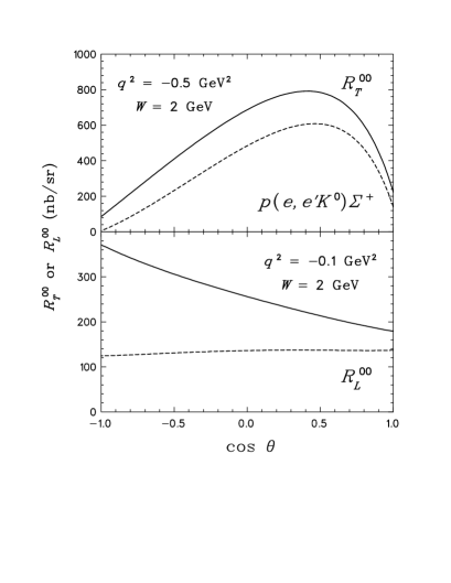
Figure 12: As in Fig. 12, but for different kinematics.

Finally, in Fig. 12 and 12 we show the sensitivities of the transverse and longitudinal response functions to different $\Sigma^{+}$ form factors in the $p(e,e^{\prime}K^{0})\Sigma^{+}$ process, in which $\Sigma^{+}$ exchange is possible. Measuring this form factor has the advantage that $\Lambda$ and $\Lambda^{*}$ exchanges are not possible in the $u$-channel, therefore eliminating some uncertainties from the hyperon transition form factor. In previous works, we have used proton form factors, scaled with the $\Sigma^{+}$ magnetic moment. We note that the CQS model predicts form factors which are very similar to those of the proton. Therefore, we compare the result only with an extreme assumption, the point $\Sigma^{+}$ approximation. Our calculations show strong sensitivities for moderate $-q^{2}$ and $\theta_{K}^{\rm cm}\geq 60^{\circ}$, which could easily be seen experimentally. Table 2 indicates that one would be able to isolate these form factors using the $R_{TL}^{0x}$ and $R_{TL}^{0y}$ observables. However, this issue can only be addressed in future works, since present elementary models still suffer from intrinsic uncertainties.

6 CONCLUSION

We have shown that kaon electroproduction on the nucleon is well suited to extract information on the form factors of strange mesons and baryons, albeit this cannot be done model-independently, like the Chew-Low extrapolation technique in the case of the charged pion and kaon. The main problem is to reduce the uncertainties in the elementary operator. This can be performed by precise experiments in kaon photoproduction where the relevant resonances and coupling constants in the process can be determined.

References

- [1] G.F. Chew and F.E. Low, Phys. Rev. 113 (1959) 1640.
- [2] Longitudinal/Transverse Cross Section Separation for , CEBAF experiment E-93-018, O.K. Baker (spokesperson).
- [3] C. Bennhold, T. Mart, and D. Kusno, Proceedings of the ICTP Conference on Perspectives in Hadronic Physics, Trieste, Italy, May 1997 (in press).
- [4] J.C. David, C. Fayard, G.H. Lamot, and B. Saghai, Phys. Rev. C 53 (1996) 2613.
- [5] G. Knöchlein, D. Drechsel, and L. Tiator, Z. Phys. A 352 (1995) 327.
- [6] R.A. Williams, C.-R. Ji, and S.R. Cotanch, Phys. Rev. C 46 (1992) 1617.
- [7] T. Mart, C. Bennhold, and C. E. Hyde-Wright, Phys. Rev. C 51 (1995) R1074.
- [8] C. Bennhold, H. Ito, and T. Mart, Proceedings of the 7th International Conference on the Structure of Baryons, Santa Fe, New Mexico, 1995, p.323.
- [9] W.W. Buck, R. Williams, and H. Ito, Phys. Lett. B 351 (1995) 24; H. Ito and F. Gross, Phys. Rev. Lett. 71 (1993) 2555.
- [10] R.A. Williams and T.M. Small, Phys. Rev. C 55 (1997) 882; R.A. Williams and C. Puckett-Truman, Phys. Rev. C 53 (1996) 1580.
- [11] H.C. Kim, A. Blotz, M. Polyakov, K. Goeke, Phys. Rev. D 53 (1996) 4013.
- [12] C.R. Münz, J. Resag, B.C. Metsch, and H.R. Petry, Phys. Rev. C 52 (1995) 2110.
- [13] Polarization Transfer in Kaon Electroproduction, TJNAF Proposal, O.K. Baker (spokesperson).